Enhanced Teaching–Learning-Based Optimization Algorithm for the Mobile Robot Path Planning Problem

Abstract

This research proposes an enhanced teaching–learning based optimization (ETLBO) algorithm to realize an efficient path planning for a mobile robot. Four strategies are introduced to accelerate the teaching–learning based optimization (TLBO) algorithm and optimize the final path. Firstly, a divide-and-conquer design, coupled with the Dijkstra method, is developed to realize the problem transformation so as to pave the way for algorithm deployment. Secondly, the interpolation method is utilized to smooth the traveling route as well as to reduce the problem dimensionality. Thirdly, an opposition-based learning strategy is embedded into the algorithm initialization to create initial solutions with high qualities. Finally, a novel, individual update method is established by hybridizing the TLBO algorithm with differential evolution (DE). Simulations on benchmark functions and MRPP problems are conducted, and the proposed ELTBO is compared with some state-of-the-art algorithms. The results show that, in most cases, the ELTBO algorithm performs better than other algorithms in both optimality and efficiency.

1. Introduction

In modern society, mobile robots have been widely introduced into the harsh manufacturing environment and some other industries to reduce labor intensity for people. Many topics associated with mobile robots have been studied, including navigation, path planning, trajectory tracking, and simultaneous localization and mapping (SLAM) [1,2,3,4]. In this regard, MRPP plays a significant role in the field of mobile robots. It is mainly responsible for finding a collision-free and optimal (or approximately optimal) traveling path [5]. This work is motivated by such a context and aims to explore a fast and efficient methodology for MRPP problems.

At present, MRPP-related algorithms mainly include the artificial potential field method, grid method, ant colony algorithm, genetic algorithm and neural network method. Due to its simple mathematical model, small computation time, and strong, real-time nature, the artificial potential field method is widely used [6]. Nevertheless, it is a local path-planning approach in nature that, considering its weaknesses of target unreachability and local minimum points, may lead to the failure of path planning. The grid method is used to model the mobile environment and then to convert the robot path into connections between grids, paving the way for algorithm deployment [7]. It is a global path-planning approach in nature. However, the number of grids increases dramatically when the mobile environment becomes larger. Thus, it is difficult to achieve the desired routes in terms of large and complex environments. In addition, some bionic intelligent optimization algorithms have been proposed and successfully applied to MRPP-related problems. Representative approaches include the ant colony algorithm (ACO), particle swarm optimization (PSO), genetic algorithm (GA), and the neural network (NN). However, it should be noted that some weaknesses of these approaches restrict their applications in MRPP, including the local optimum, low search efficiency, and large burden of computation [8,9,10]. Therefore, this work focuses on designing a more efficient procedure and methodology to generate solutions for MRPP problems.

In real-world applications, major efforts have concentrated on strengthening by hybridizing one candidate bionic intelligent optimization algorithm with other sophisticated skills. The ACO is one example: some of the most recent ACO-based path-planning algorithms are reviewed as follows. To reduce search blindness, Zhao et al. [11] embedded the directional, heuristic information and unevenly distributed initial pheromone into the ACO architecture. The rollback strategy was introduced by Wu et al. [12] to make more ants reach the goal, and the death strategy was also utilized to reduce the influence of an invalid pheromone on the algorithm evolution. Wang et al. [13] designed an improved, pseudo-random proportional rule for the ant state transition which greatly improved the convergence speed. A novel penalty strategy to volatilize the poor path pheromone was embedded into the ACO by Yue et al. [14], which efficiently improved the utilization rate of the ant exploration. Chen et al. [15] tried to improve the visibility of heuristic information by virtue of the principle of infinite step length. In addition, the pheromone update rules, as well as the evaporation rate, were dynamically adjusted to accelerate the convergence speed. The evaluation function of the A-star algorithm and the curvature suppression operator were introduced into the ACO by Dai et al. [16]; these additions were in favor of accelerating the convergence and improving the smoothness of the final path. Luo et al. [17] proposed an attenuation-factor-based heuristic information mechanism, and adjusted the pseudo-random ratio of state selection by means of an adaptive function. The adaptive adjustment factor and pheromone volatilization factor were embedded into the pheromone update rule by Miao et al. [18]. Such modifications efficiently balanced the global search ability and convergence. As can be noted from the above literature, different skills have been embedded into the basic algorithm with respect to the aspects of path formulation, path adjustment, solution modification, individual update, etc. The proposed ETLBO is motivated and designed by these observations and is developed by virtue of TLBO.

Many practical applications have proven TLBO to be superior to some conventional metaheuristics [19,20,21]. TLBO simulates the behaviors of the teacher and students in the classroom, where the so-called teacher and learner phases are utilized to update the population in the algorithm evolution. Some modified, TLBO-related algorithms have already been proposed by many researchers; please refer to the book by Rao [22] for the most recent studies. However, some challenges still exist when applying the TLBO approach to practical optimization problems [23]. First, the adaptation of TLBO to a specified application requires an appropriate problem conversion and solution representation. Second, TLBO tends to get trapped in a local optimum in real-world applications, which is a common weakness of swarm-based metaheuristics. In this context, this paper develops an efficient, TLBO-based algorithm for MRPP.

This work is motivated by the great demand for a fast and efficient path-planning approach for a mobile robot in a complex environment. In the current research, an effort is made to address such an issue with a TLBO-version approach. Four main contributions associated with the methodology design are stated as follows:

• For the algorithm deployment, a divide-and-conquer design, coupled with the Dijkstra method, is developed to realize the problem transformation;
• The interpolation method is embedded into the proposed algorithm to smooth the traveling route as well as to reduce the problem dimensionality;
• An opposition-based learning strategy is utilized to modify the algorithm initialization process;
• To balance between exploitation and exploration, a novel, individual update method is established by hybridizing TLBO with DE.

The rest of this work is organized as follows. Section 2 formulates the MRPP, and Section 3 presents a brief introduction of TLBO and DE. The proposed methodology is formally described in Section 4. Computational studies are designed and carried out in Section 5. Finally, Section 6 displays conclusions and future work.

2. Problem Formulation

This section models the investigated MRPP problem by virtue of the grid environment map, and then formulates it with the objective of minimizing the route length.

2.1. Problem Description

As is illustrated in Figure 1, a two-dimension grid map was utilized to model the environment so that the coordinate information of each grid can be easily computed with the predefined grid size, $a$. In this regard, the robot path between the origin and destination can be expressed by a series of connections between different grids.

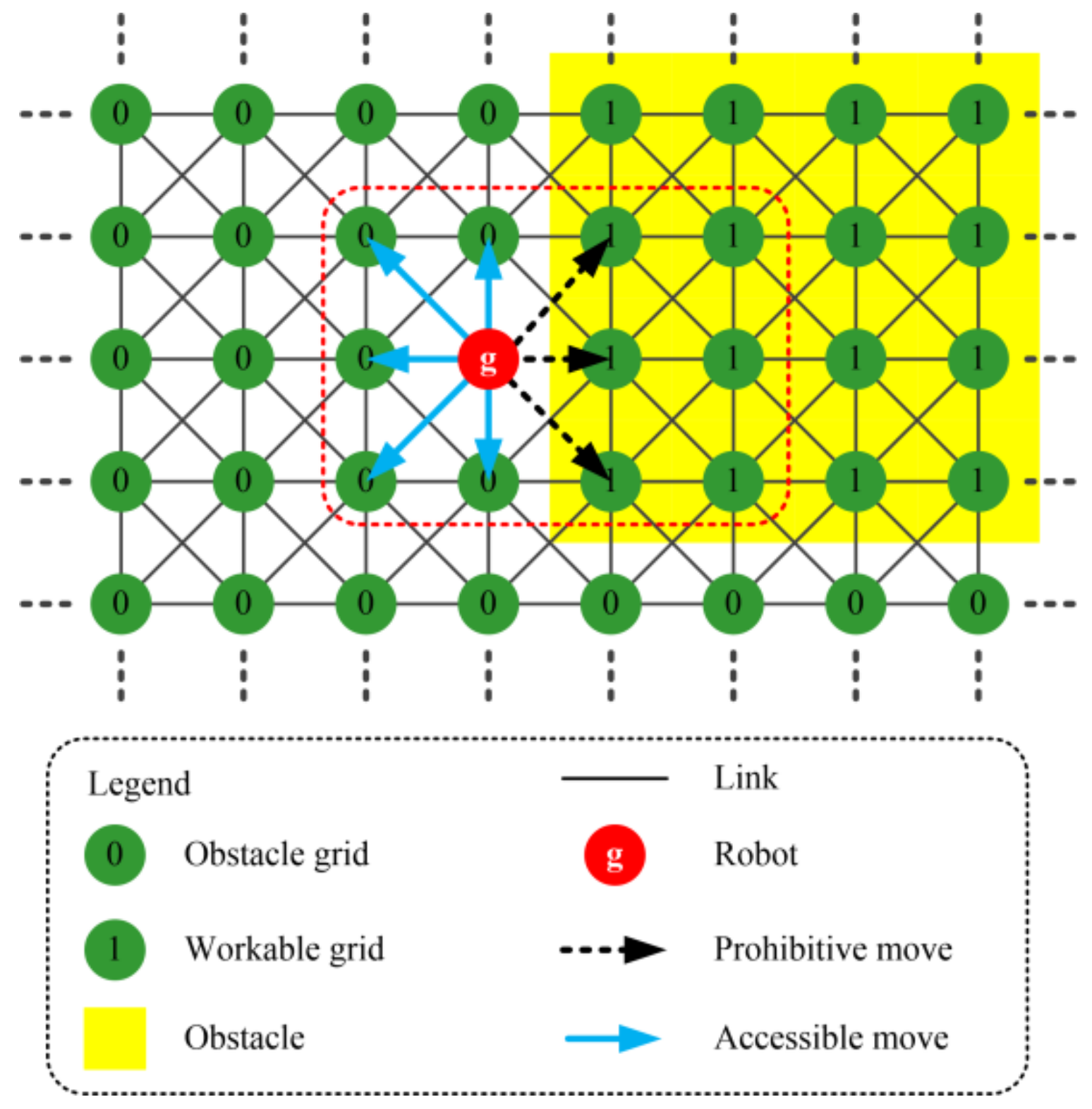
Figure 2 is employed here to better illustrate the move rules of the grid map. When placed at a specified grid, the robot can only move to, at most, eight adjacent workable grids. Let notation $g_i$ represent the robot’s current position and set $\mathsf{\Omega }$ to denote all workable girds. All possible reachable positions of grid $g_i$ can be stated as follows:

$$N(g_i)=\left\{g_j\left|\begin{array}{c}a\le d(g_i,g_j)\le \sqrt{2}\cdot a\\ \hspace{0.33em}{g}_j\in \mathsf{\Omega }\end{array}\right.\right\}$$

(1)

where $d(g_i,g_j)$ represents the distance value between any two grids, $g_i$ and $g_j$.

2.2. Mathematical Model

The investigated MRPP aims to find a set of optimal grid connections between the origin and destination so that some numerical metrics can be optimized or improved. Two constraints should be obeyed during the whole decision process: namely, the continuity constraint and the obstacle-avoidance constraint. The previous constraint requires that the robot must start from the origin, move to adjacent grids step by step, and finally reach its destination. The latter states that obstacle grids are not allowed to be included in the robot path.

This research formulated the considered problem with the objective of minimizing the total route length. Given a robot route $S=\left\{g_i|i=1,2,\dots \dots ,n\right\}$, the objective definition is as follows:

$$\min L={\displaystyle \sum _{i=1}^{n}d(g_i,g_{i+1})}$$

(2)

where $n$ is the total number of grids in the robot route.

3. TLBO and DE Algorithms

The proposed ETLBO under study capitalizes on the strengths of both TLBO and DE to form a novel and efficient hybrid algorithm.

3.1. TLBO

TLBO simulates the teaching–learning phenomenon in a classroom to solve complicated optimization problems with appreciable efficiency. It is a swarm-based evolutionary algorithm that utilizes a group of so-called individuals to produce a global optimum. In TLBO, the current best solution is considered to be the teacher individual, and the other solutions are treated as student individuals. A group of solutions are created in a random way. They then evolve by two fundamental modes of learning: namely, the teacher phase and the learner phase. The classical TLBO is executed through the following steps:

• Step 1. Initialize the parameter settings, including the population size, $P$, maximum iteration, $G$, problem dimension, $D$, etc.;
• Step 2. Create initial individuals then calculate their objective values;
• Step 3. Employ the teacher phase to update the current population;
• Step 4. Employ the learner phase to update the current population;
• Step 5. If any algorithm termination criterion is satisfied, terminate the search process and output the current best individual; otherwise, go to Step 3.

Detailed mathematical formulations of TLBO are stated as follows.

(1)

Initial phase

The solution in TLBO is expressed by an array, $x=(x_1,x_2,\cdots ,x_d,\cdots ,x_D)$, in which $d\in \{1,2,\cdots ,D\}$. Given a variable range, $[x_d^l,x_d^u]$, $P$ random individuals are initialized by the following equation:

$$x_d=x_d^l+rand(0,1)\cdot \left(x_d^u-x_d^l\right)$$

(3)

where $rand(0,1)$ is a uniform random number in the interval [0, 1].

(2)

Teacher phase

The mean position of the current population is calculated. Let $\overline{x}=({\overline{x}}_1,\cdots ,{\overline{x}}_d,\cdots ,{\overline{x}}_D)$ be the mean solution, and $x^{\ast }$ represents the current best solution. The teacher phase is implemented based on the position difference between $\overline{x}$ and $x^{\ast }$. In this regard, the equation is stated as follows:

$$x^{\prime }=x+rand(0,1)\cdot \left(x^{\ast }-\partial \cdot \overline{x}\right)$$

(4)

where parameter $\partial$ is the teaching factor that lies in the set {1, 2}. If the mutant individual performs better than its parent, a greedy selection is then introduced, and $x$ would be replaced by $x^{\prime }$.

(3)

Learner phase

The learner phase is implemented based on the position difference between the current solution and one randomly selected individual. Let $f(\cdot )$ represent the objective function formula. The offspring is produced as follows:

$$x^{\prime }=\left\{\begin{array}{ll}x+rand(0,1)\cdot (x^1-x)\hfill & \mathrm{if}\hspace{0.33em}f(x^1)<f(x^2)\hfill \\ x+rand(0,1)\cdot (x^2-x)\hfill & \mathrm{otherwise}\hfill \end{array}\right.$$

(5)

where $x^1$ and $x^2$ denote two randomly selected individuals. In addition, the greedy selection is applied in an analogous way to the teacher phase.

3.2. DE

The DE approach is a stochastic and swarm-based optimization algorithm [24]. It begins with a random initial population consisting of a number of target individuals. The population evolves by means of mutation and crossover and selection operators. The detailed operations of a classical DE are as follows:

(1)

Mutation operation

The mutation operation in the DE approach is utilized to generate a mutant vector associated with each target individual in the current population. Given a candidate solution, $x$, its associated mutant vector, $v$, can be produced by taking one of the following strategies.

$$\begin{array}{}\mathrm{(6)}& \mathrm{DE}/\mathrm{rand}/1 v=x_{r_1}+F\cdot (x_{r_2}-x_{r_3})\mathrm{(7)}& \mathrm{DE}/\mathrm{rand}/2 v=x_{r_1}+F\cdot (x_{r_2}-x_{r_3})+F\cdot (x_{r_4}-x_{r_5})\mathrm{(8)}& \mathrm{DE}/\mathrm{best}/1 v=x_{best}+F\cdot (x_{r_2}-x_{r_3})\mathrm{(9)}& \mathrm{DE}/\mathrm{best}/2 v=x_{best}+F\cdot (x_{r_2}-x_{r_3})+F\cdot (x_{r_4}-x_{r_5})\mathrm{(10)}& \mathrm{DE}/\mathrm{current}-\mathrm{to}-\mathrm{best}/1 v=x+F\cdot (x_{best}-x)+F\cdot (x_{r_1}-x_{r_2})\end{array}$$

where $x_{r_1}~x_{r_5}$ are randomly selected individuals and $x_{best}$ represents the current best solution. Meanwhile, the scaling factor, $F$, is used to control the differential variation between two individuals.

(2)

Crossover operation

The DE algorithm employs a crossover operation to generate candidate offspring in order to the increase population diversity. In this regard, a candidate offspring, $u$, is produced by combing solution information from each pair of a target vector, $x$, and its associated mutant vector, $v$. The scheme can be described as follows:

$$u_d=\left\{\begin{array}{ll}{v}_d& \hfill rand(0,1)\le CR\hfill \\ x_d& \hfill \mathrm{otherwise}\hfill \end{array}\right.$$

(11)

where $d\in \{1,2,\cdots ,D\}$, and $rand(0,1)$ is a random number in the interval $[0,1]$. Symbols $x_d$, $v_d$, and $u_d$ represent the $d-\mathrm{th}$ gene in the individual vectors $x$, $v$, and $u$, respectively. The crossover probability, $CR$, is utilized to control the proportion of genes copied from target and mutant vectors.

(3)

Selection operation

The selection operation in the DE algorithm employs a one-to-one greedy selection to determine whether the candidate offspring, $u$, can replace its parent individual, $x$. Solution $x$ will be replaced by $u$ once that $u$ performs equally or even better than $x$.

4. Proposed ETLBO for MRPP

This section presents a detailed introduction of the proposed methodology for the MRPP problem.

4.1. Divide-and-Conquer Design for MRPP

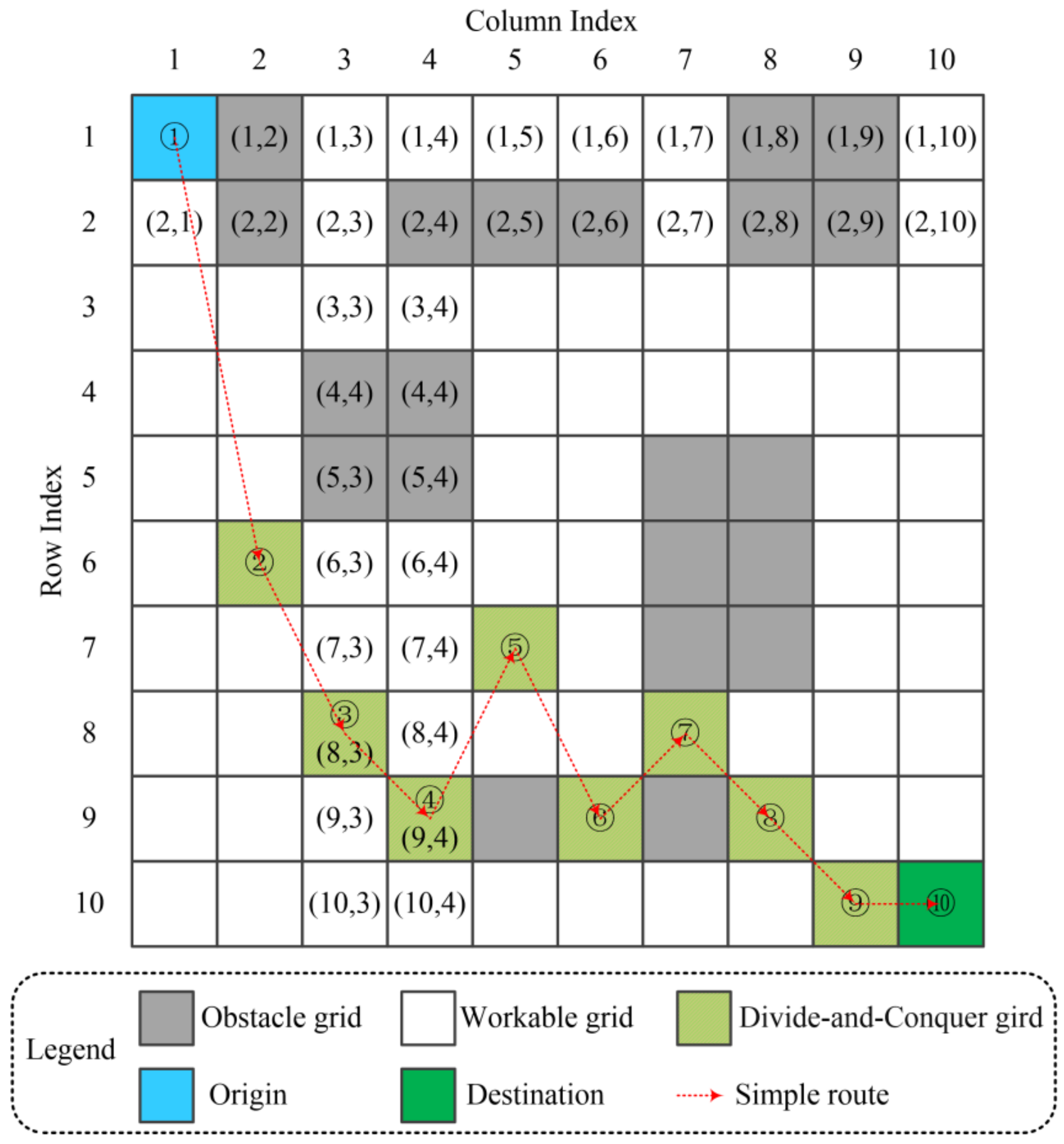
As is illustrated in Figure 3, a divide-and-conquer design is embedded into the algorithm deployment. In this regard, the investigated MRPP problem is broken down into multiple simple sub-problems, for which an appropriate divide-and-conquer grid in each column between the origin and destination must be optimized to form a simple route [25]. Then, local optimal routes between any two divide-and-conquer grids are generated by fast and sophisticated methods to form a solution to the original MRPP problem.

Two decisions must be made when dealing with the converted problem. First, an appropriate divide-and-conquer grid in each column between the origin and destination must be determined in order to construct the simple route. Second, local optimal routes between any two divide-and-conquer grids must be obtained to form a solution to the original MRPP problem. The prior decision is to be tackled by the proposed ETLBO, while the latter decision is optimized by the Dijkstra approach. More details are presented here to better explain the application of the Dijkstra approach. Let us denote the grid in a (row, column) format. For example, (1, 3) represents the grid located at row 1 and column 3. On this basis, all workable grids in column 3 and column 4 can be expressed by sets A = {(1, 3), (2, 3), (3, 3), (6, 3), (7, 3), (8, 3), (9, 3), (10, 3)} and B = {(1, 4), (3, 4), (6, 4), (7, 4), (8, 4), (9, 4), (10, 4)}, respectively. The Dijkstra approach is then utilized to obtain optimal routes between any two positions from sets A and B, respectively. Since these positions are located in columns adjacent to each other, the decision process of the Dijkstra approach is time-saving and always ensures optimality.

4.2. Interpolation Application in ETLBO

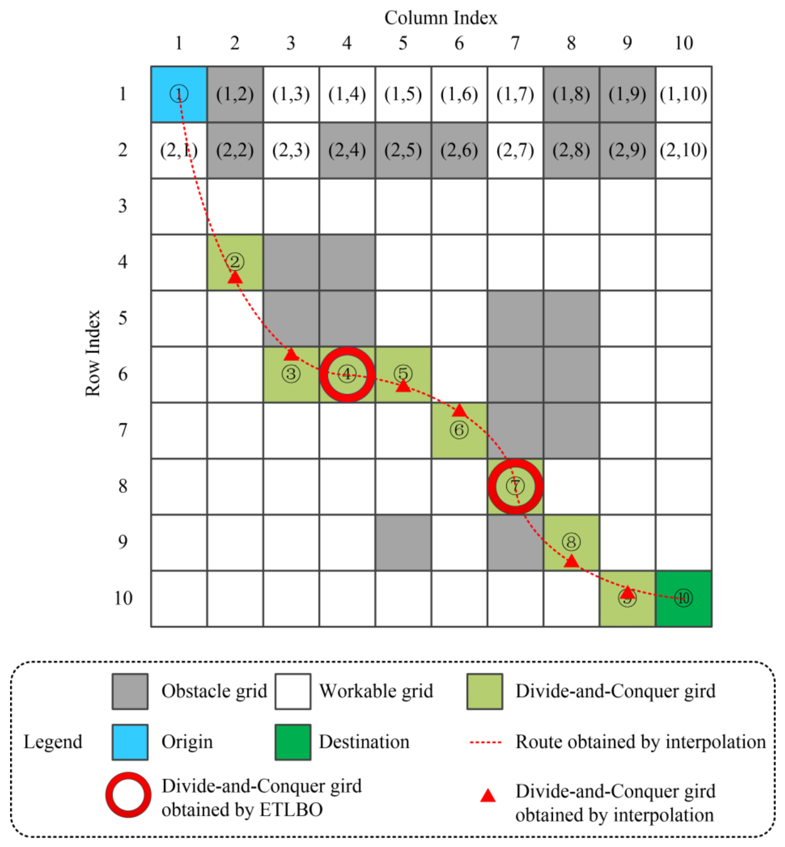
As stated in the previous subsection, ETLBO is used to determine the locations of every divide-and-conquer grid at each column between the origin and destination. To reduce the problem dimensionality and to smooth the traveling routes, the interpolation method is embedded into the application of the ETLBO. The corresponding illustrative schematic diagram is depicted in Figure 4.

It can be observed from Figure 4 that some divide-and-conquer grids are to be optimized by the solution array of the ETLBO, such as grids ④ and ⑦, while the other divide-and-conquer grids are obtained by the interpolation method. In the case in which an interpolated grid is located at an obstacle grid, the nearest workable grid in that column is selected as the divide-and-conquer grid. In this regard, the B-Spline interpolation method is selected to pave the way for ELTBO deployment according to some existing MRPP-related studies [26].

4.3. Pyramid of ETLBO

ETLBO is established by virtue of the outstanding performance of TLBO. Meanwhile, the opposition-based learning mechanism and the DE-related offspring method are utilized to enhance the algorithm performance.

4.3.1. Opposition-Based Learning Initialization Method

The opposition-based learning mechanism is a simple but efficient method to strengthen the algorithm’s performance in swarm computation [27]. In ETLBO, the opposition-based learning mechanism is used to create intimal solutions with high qualities. In this regard, $P$ solutions are initialized in a random way. Then, $P$ opposition-based solutions are generated based on the opposition-based learning concept. Finally, $P$ individuals with better evaluations are selected to form the initial population.

As stated previously, TLBO is run by virtue of $P$ individuals, and each candidate can be marked as an array $x=(x_1,x_2,\cdots ,x_d,\cdots ,x_D)$ in which $d\in \{1,2,\cdots ,D\}$. In this regard, the search space is defined by $[x_d^l,x_d^u]$. In the initialization, let us denote the $i-\mathrm{th}$ random solution and its associated, opposition-based solution by $x^{p,i}=(x_1^{p,i},\cdots ,x_d^{p,i},\cdots ,x_D^{p,i})$ and $x^{o,i}=(x_1^{o,i},\cdots ,x_d^{o,i},\cdots ,x_D^{o,i})$, respectively. According to “Definition 2” stated by Mahdavi et al. [27], the following formula holds true:

$$x_d^{o,i}=x_d^l+x_d^u-x_d^{p,i}$$

(12)

Based on the above concepts, the initialization process in ETLBO is implemented as follows:

• Step 1. Set $i\leftarrow 1$ and $d\leftarrow 1$. Then, go to step 2.
• Step 2. If condition $i\le P$ holds, go to step 3; otherwise, go to step 7;
• Step 3. If condition $d\le D$ holds, go to step 4; otherwise, go to step 5;
• Step 4. Set $x_d^{p,i}=x_d^l+rand(0,1)\cdot (x_d^u-x_d^l)$ and $x_d^{o,i}=x_d^l+x_d^u-x_d^{p,i}$. Then, go to step 5;
• Step 5. Set $d\leftarrow d+1$, if condition $d>D$ holds, go to step 6; otherwise, go to step 3;
• Step 6. Set $i\leftarrow i+1$; then, go to step 2;
• Step 7. Select $P$ best individuals from $\{x^{p,1},\cdots ,x^{p,P},x^{o,1},\cdots ,x^{o,P}\}$ to form the initial population.

4.3.2. Hybrid Offspring Generation Method

An efficient swarm-based metaheuristic should make full use of both the local and global information on the solutions found. Local information on solutions can be helpful for exploitation, while global information tends to guide the search for exploring promising areas. The evolution of TLBO mainly depends on the global information, and thus TLBO has an obvious advantage in that learner individuals will converge at a single attractor/teacher individual. It can be observed that DE evolves mainly based on the distance and direction information, which are types of local information in nature. In other words, DE has the advantage of not being biased toward any prior defined guide, and such an attribute makes DE able to maintain population diversity and explore local searches.

The key reason for employing the hybridization of different metaheuristics is that the hybrid approach can make full use of the strengths of each algorithm while simultaneously overcoming the associated limitations. In this regard, instead of employing a single updated learner individual in the TLBO, the proposed ETLBO makes use of the integration of two offspring individuals. The first offspring individual is computed by the TLBO, and the second one is obtained by the DE operators. Detailed mathematical expressions are described as follows.

(1)

Teacher phase

Given a candidate solution, $x$, the corresponding offspring individual, $x^{\prime }$, is calculated by the hybridization of the teacher phase in TLBO and differential learning in DE:

$$x^{\prime }=u_1\cdot x^{TLBO,Teach}+(1-u_1)\cdot x^{DE,Teach}$$

(13)

where $x^{TLBO,Teach}$ represents the offspring individual obtained by Equation (4) in TLBO, while $x^{DE,Teach}$ represents the offspring individual computed by Equations (6)–(11) in DE. The hybridization factor $u_1$ is a random number that lies in the interval [0, 1].

(2)

Learner phase

Analogous to the teacher phase, the offspring individual $x^{\prime }$ of a candidate solution $x$ is generated by taking the following equation:

$$x^{\prime }=u_2\cdot x^{TLBO,Learn}+(1-u_2)\cdot x^{DE,Learn}$$

(14)

where $x^{TLBO,Learn}$ represents the offspring individual obtained by Equation (5) in TLBO, while $x^{DE,Learn}$ is the offspring individual computed by Equations (6)–(11) in DE. The hybridization factor $u_2$ is a random number that lies on interval [0, 1].

4.4. Framework of Proposed Methodology for MRPP

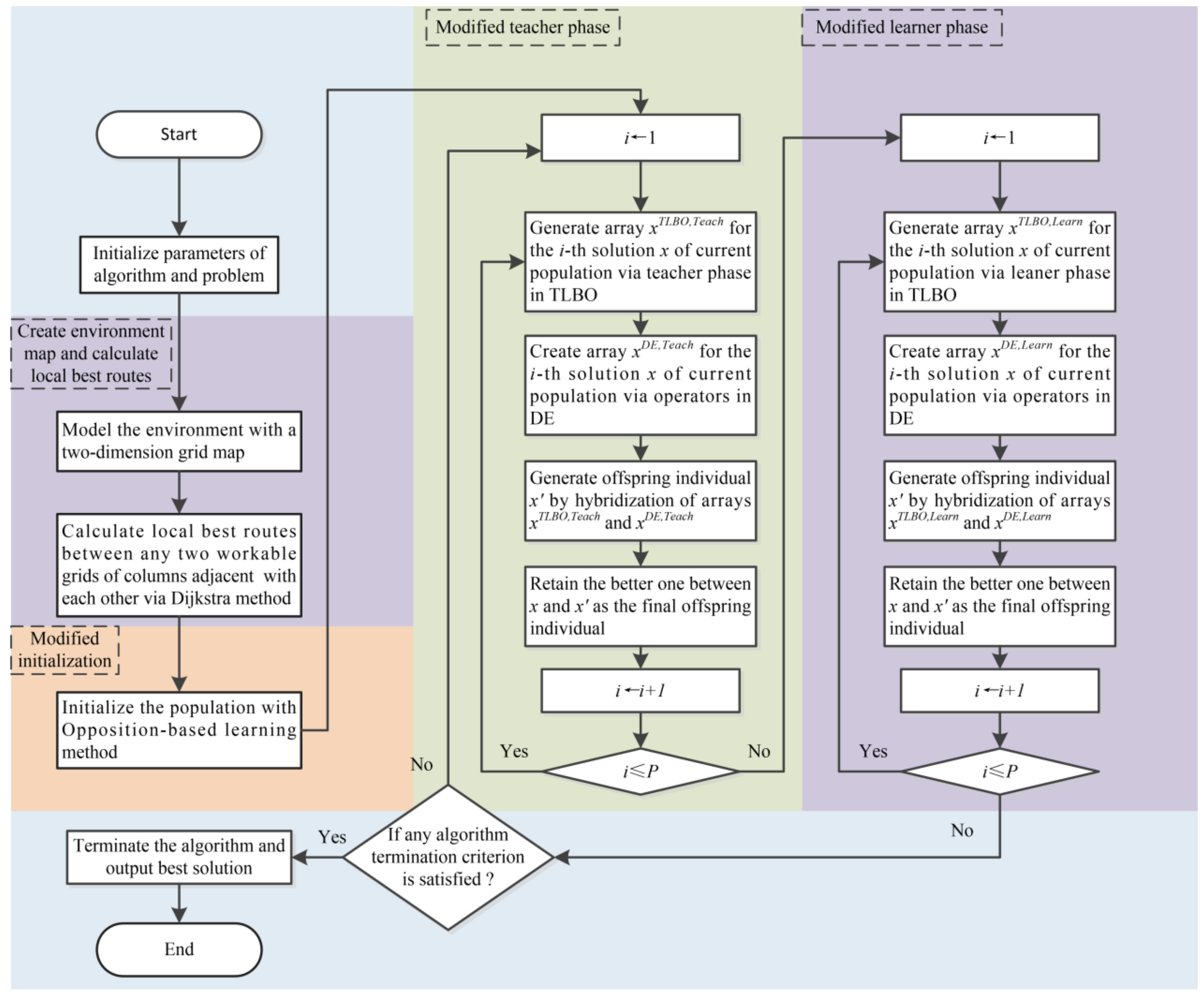
By virtue of the previous statements, the flowchart of the proposed ETLBO for the MRPP problem is illustrated in Figure 5. Simulations are to be conducted in the next section to validate the algorithm performance.

5. Experimental Studies

Simulation experiments on the benchmark functions and MRPP problems were designed and carried out to validate the proposed methodology. All experiments were performed on a MATLAB 2016b platform, using a personal computer with a 2.4 GHz Intel Core i5 CPU and 4 GB of RAM.

5.1. Benchmark Function Problem

In this subsection, the ETLBO is validated by virtue of 20 benchmark function problems which are commonly used to evaluate new optimization methods. These functions can be classified according to several criteria, such as their linearity (or nonlinearity), convexity (or non-convexity), and continuousness (or non-continuousness). However, unimodal (or multimodal), separable (or non-separable), and dimensionality characteristics are of great importance for benchmark functions to evaluate the algorithm efficiency. Unimodal functions increase and decrease monotonically, while multimodal functions have two or more vague peaks. Separable functions are easier to resolve when compared to non-separable functions. Regarding the problem dimensionality, its increase also raises the optimization difficulty. In this context, this work employed benchmark functions with combinations of different characteristics to evaluate the proposed ETLBO.

5.1.1. Preliminaries

A. 

Unimodal functions

Table 1. Unimodal benchmark functions.

Label	Name	Formula	Range	Dimension	Optimum
F1	Sphere	$f_1(x)={\displaystyle \sum _{i=1}^n{x}_i^2}$	[−100, 100]	100	0
F2	Step	$f_6(x)={\left(\left[x_i+0.5\right]\right)}^2$	[−100, 100]	30	0
F3	Quartic	$f_7(x)={\displaystyle \sum _{i=1}^{n}i{x}_i{}^4+rand\left(0,1\right)}$	[−1.28, 1.28]	30	0
F4	Schwefel 2.21	$f_4(x)=\max x_i\left\{\left|x_i\right|\right.,\left.1\le i\le n\right\}$	[−100, 100]	60	0
F5	Booth	$f_5(x)={(x_1+2x_2-7)}^2+{(2x_1+x_2-5)}^2$	[−10, 10]	2	0
F6	Schwefel 2.22	$f_2(x)={\displaystyle \sum _{i=1}^n\left|x_i\right|}+{\displaystyle \prod _{i=1}^n\left|x_i\right|}$	[−10, 10]	40	0
F7	Schwefel 1.2	$f_3(x)={{\displaystyle \sum _{i=1}^n\left({\displaystyle \sum _{j-1}^i{x}_j}\right)}}^2$	[−100, 100]	50	0
F8	Easom	$f_8(x)=-\cos (x_1)\cos (x_2)\exp (-{(x_1-\pi )}^2-{(x_2-\pi )}^2)$	[−100, 100]	2	−1
F9	Bohachevsky	$f_{14}(x)=x_1^2+2x_2^2-0.3\cos (3\pi x_1)-0.4\cos (4\pi x_2)+0.7$	[−100, 100]	2	0
F10	Matyas	$f_{17}(x)=0.26\left(x_1^2+x_2^2\right)-0.48x_1{x}_2$	[−10, 10]	2	0
F11	Three-hump camel	$f_{18}(x)=2x^2-1.05x^4+\frac{x^6}{6}+xy+y^2$	[−5, 5]	2	0
F12	Schaffer N.2	$f_{20}(x)=0.5+\frac{{\sin }^2\left(x^2-y^2\right)-0.5}{{\left[1+0.001\left(x^2+y^2\right)\right]}^2}$	[−100, 100]	2	0

summarizes the unimodal functions utilized in this study. In this regard, the search space, problem dimension, and optimum for 12 benchmark functions, F1–F12, are presented [28]. Functions F1–F3 were separable, and functions F4–F12 were non-separable. The complexity expanded with increasing problem dimensions, which varied up to a maximum value of 100.

B. 

Multimodal functions

Multimodal functions F13–F20 were employed for the algorithm evaluation in this work [29]. Functions F13–F14 were separable, while functions F15–F20 were non-separable. The multimodal functions employed here are detailed in

Table 2. Multimodal benchmark functions.

Label	Name	Formula	Range	Dimension	Optimum
F13	Rastrigin	$f_9(x)={\displaystyle \sum _{i=1}^n\left[x_i^2-10\cos \left(2\pi x_i\right)+10\right]}$	[−5.12, 5.12]	20	0
F14	Branin	$f_{15}(x)={\left(x_2-\frac{5.1}{4{\pi }^2}{x}_1^2+\frac{5}{\pi }{x}_1-6\right)}^2+10\left(1-\frac{8}{\pi }\right)\cos x_1+10$	[−5, 15]	2	0.398
F15	Ackley	$f_{10}(x)=-20\exp \left(-0.2\sqrt{\frac{1}{n}}{\displaystyle \sum _{i=1}^n{x}_i^2}\right)-\exp \left(\frac{1}{n}{\displaystyle \sum _{i=1}^n\cos \left(2\pi x_i\right)}\right)+20+e$	[−32.32]	30	0
F16	Griewank	$f_{11}(x)=\frac{1}{4000}{\displaystyle \sum _{i=1}^n{x}_i^2}-{\displaystyle \prod _{i=1}^n\cos \left(\frac{x_i}{\sqrt{i}}\right)}+1$	[−600, 600]	30	0
F17	Penalized	$\begin{array}{l}{f}_{12}(x)=\frac{\pi }{n}\left\{10{\sin }^2\left(\pi y_i\right)+{\displaystyle \sum _{i=1}^{n-1}{\left(y_i-1\right)}^2\left[1+10{\sin }^2\left(\pi y_{i+1}\right)+{\left(y_i-1\right)}^2\right]}\right\}+{\displaystyle \sum _{i=1}^{n}u\left(x_i,10,100,4\right)}\\ y_i=1+\frac{x_i+1}{4}\\ u\left(x_i.a,k,m\right)=\left\{\begin{array}{l}k{\left(x_i-a\right)}^m;x_i>a\\ 0;-a<x_i<a\\ k{\left(-x_i-a\right)}^m;x_i<-a\end{array}\right.\\ \end{array}$	[−50, 50]	50	0
F18	Penalized2	$\begin{array}{l}{f}_{13}(x)=0.1\left\{{\sin }^2\left(3\pi x_1\right)+{\displaystyle \sum _{i=1}^{n-1}{\left(x_i-1\right)}^2\left[1+{\sin }^2\left(3\pi x_{i-1}\right)\right]+{\left(x_n-1\right)}^2\left[1+{\sin }^2\left(2\pi x_n\right)\right]}\right\}+{\displaystyle \sum _{i=1}^{n}u\left(x_i,10,100,4\right)}\\ u\left(x_i.a,k,m\right)=\left\{\begin{array}{l}k{\left(x_i-a\right)}^m;x_i>a\\ 0;-a<x_i<a\\ k{\left(-x_i-a\right)}^m;x_i<-a\end{array}\right.\\ \end{array}$	[−50, 50]	30	0
F19	Goldstein-Price	$f_{16}(x)=\left[1+{\left(x_1+x_2+1\right)}^2\left(19-14x_1+3x_1^2-14x_2+6x_1{x}_2+3x_2^2\right)\right]\ast \left[30+{\left(2x_1-3x_2\right)}^2\left(18-32x_1+12x_1^2+48x_2-36x_1{x}_2+27x_2^2\right)\right]$	[−2, 2]	2	3
F20	Levi	$f_{19}(x)={\sin }^2\left(3\pi x\right)+{\left(x-1\right)}^2\left(1+{\sin }^2\left(3\pi y\right)\right)+{\left(y-1\right)}^2\left(1+{\sin }^2\left(2\pi y\right)\right)$	[−10, 10]	2	0

with their related search space, problem dimension, and optimum.

C. 

Evaluation metrics

To evaluate the algorithm performance, some metrics were calculated based on 50 independent runs. The metrics utilized in this subsection included the best, worst, median, average, and standard deviation (SD) values, computed according to 50 independent runs of each benchmark function.

D. 

Non-parametric tests

Non-parametric tests are statistical analysis experiments for sample data that do not require the underlying population for assumptions. This work employed the Wilcoxon rank-sum test to validate the algorithm performance for different test functions [30]. In this regard, the rankings of the sample data were allotted by combining two populations. Since all functions were considered minimization problems, observations in two populations were first sorted in ascending order, and the Wilcoxon rank-sum statistics were then calculated in the following manner:

$$w_A={\displaystyle \sum _{r\in R_A}r}$$

(15)

where $w_A$ is the sum of rank values in population A.

In addition, in a Wilcoxon rank-sum test for the comparison of two candidate algorithms, the null hypothesis and the alternate hypothesis can be stated as follows: H0: population A ≥ population B; Ha: population A < population B. In this regard, the related $p$ value is given by:

$$p=\left\{\begin{array}{cc}\mathrm{Pr}(W_A\ge w_A)& Ha:A>B\\ \mathrm{Pr}(W_A\le w_A)& Ha:A<B\end{array}\right.$$

(16)

where $W_A$ represents the distribution of the rank sum. The resulting $p$ is compared to the so-call significance level, which is set to 0.05 in the current study.

5.1.2. Results and Discussion

Simulations were carried out to compare the solution performance of ETLBO with some well-known and state-of-art methods, including TLBO, TLBO(S) (an enhanced TLBO proposed by Shukla et al.) [31], PSO, DE, and GA. According to some related studies and tentative experiments, the population size and maximum iteration of all test algorithms were set as 50 and 5000, respectively. For ETLBO, the scaling factor, $F$, was set to 0.4 and the crossover probability, $CR$, was fixed at 0.8. Other parameters of compared algorithms were set to values recommended by the related literature. For the sake of constancy, the simulation of a test algorithm for each benchmark function was exacted 50 independent times. The results are presented and discussed as follows.

A. 

Results of unimodal functions

Table 3. Simulation results of unimodal functions.

Algorithm	Metric	ETLBO	TLBO	TLBO(S)	PSO	DE	GA
F1	Best	1.41 × 10−134	1.11 × 10−11	7.31 × 10−20	1.44 × 1001	4.61 × 1000	4.07 × 1002
	Worst	3.35 × 10−129	1.47 × 10−11	2.81 × 10−11	1.59 × 1002	6.83 × 1000	9.34 × 1002
	Median	1.92 × 10−132	1.40 × 10−11	1.72 × 10−14	1.59 × 1001	5.73 × 1000	5.59 × 1002
	Average	1.19 × 10−130	1.32 × 10−11	1.16 × 10−12	2.79 × 1001	5.72 × 1000	5.65 × 1002
	SD	5.04 × 10−130	8.61 × 10−13	4.21 × 10−12	3.36 × 1001	5.11 × 10−01	9.93 × 1001
F2	Best	0.00 × 1000	0.00 × 1000	0.00 × 1000	2.70 × 10−23	0.00 × 1000	0.00 × 1000
	Worst	0.00 × 1000	0.00 × 1000	0.00 × 1000	4.46 × 10−15	0.00 × 1000	0.00 × 1000
	Median	0.00 × 1000	0.00 × 1000	0.00 × 1000	1.90 × 10−20	0.00 × 1000	0.00 × 1000
	Average	0.00 × 1000	0.00 × 1000	0.00 × 1000	9.13 × 10−17	0.00 × 1000	0.00 × 1000
	SD	0.00 × 1000	0.00 × 1000	0.00 × 1000	6.23 × 10−10	0.00 × 1000	0.00 × 1000
F3	Best	1.29 × 10−07	4.80 × 10−01	7.70 × 10−05	2.45 × 10−02	2.50 × 10−02	1.43 × 10−02
	Worst	1.75 × 10−04	6.76 × 10−01	1.01 × 10−02	5.40 × 10−02	8.61 × 10−02	1.13 × 10−01
	Median	2.95 × 10−05	6.17 × 10−01	1.41 × 10−03	5.23 × 10−05	5.20 × 10−02	3.90 × 10−02
	Average	4.40 × 10−05	6.12 × 10−01	2.15 × 10−03	8.61 × 10−02	5.54 × 10−02	4.22 × 10−02
	SD	3.85 × 10−05	3.66 × 10−02	1.86 × 10−03	1.30 × 10−02	1.48 × 10−02	1.84 × 10−02
F4	Best	0.00 × 1000	4.72 × 10−09	1.00 × 10−16	2.19 × 10−01	1.00 × 1001	1.18 × 1001
	Worst	0.00 × 1000	6.11 × 10−09	2.62 × 10−13	1.56 × 1000	1.61 × 1001	3.07 × 1001
	Median	0.00 × 1000	5.37 × 10−09	1.60 × 10−14	7.17 × 10−01	1.38 × 1001	1.88 × 1001
	Average	0.00 × 1000	5.35 × 10−09	3.57 × 10−14	8.01 × 10−01	1.35 × 1001	1.97 × 1001
	SD	0.00 × 1000	3.27 × 10−10	5.11 × 10−14	3.82 × 10−01	1.38 × 1000	3.76 × 1000
F5	Best	0.00 × 1000	2.00 × 1000	8.37 × 10−08	0.00 × 1000	0.00 × 1000	2.07 × 10−03
	Worst	2.15 × 10−04	2.00 × 1000	2.30 × 10−01	0.00 × 1000	0.00 × 1000	1.91 × 1000
	Median	3.74 × 10−16	2.00 × 1000	1.64 × 10−02	0.00 × 1000	0.00 × 1000	6.00 × 10−01
	Average	8.05 × 10−06	2.00 × 1000	2.30 × 10−02	0.00 × 1000	0.00 × 1000	9.45 × 10−01
	SD	3.00 × 10−05	4.35 × 10−09	4.97 × 10−02	0.00 × 1000	0.00 × 1000	8.29 × 10−01
F6	Best	0.00 × 1000	9.76 × 10−03	1.31 × 10−08	5.01 × 10−06	1.72 × 10−03	1.39 × 10−02
	Worst	0.00 × 1000	3.79 × 10−01	1.19 × 10−05	1.36 × 10−01	3.69 × 10−03	9.86 × 10−02
	Median	0.00 × 1000	1.35 × 10−01	6.33 × 10−07	4.43 × 10−04	2.57 × 10−03	3.73 × 10−02
	Average	0.00 × 1000	1.60 × 10−01	2.01 × 10−06	4.13 × 10−03	2.69 × 10−03	4.04 × 10−02
	SD	0.00 × 1000	8.19 × 10−02	2.71 × 10−06	1.81 × 10−02	4.34 × 10−04	1.72 × 10−02
F7	Best	2.69 × 10−170	2.50 × 10−19	1.93 × 10−11	1.27 × 1003	7.34 × 1004	5.14 × 1003
	Worst	1.65 × 10−155	2.12 × 10−10	8.55 × 10−21	9.14 × 1003	1.25 × 1005	2.20 × 1004
	Median	4.25 × 10−163	2.13 × 10−14	1.78 × 10−11	3.99 × 1003	1.08 × 1005	9.40 × 1003
	Average	3.29 × 10−157	6.85 × 10−12	9.30 × 10−11	4.43 × 1003	1.03 × 1005	1.05 × 1004
	SD	2.17 × 10−156	3.24 × 10−11	9.32 × 10−11	1.79 × 1003	1.24 × 1004	3.66 × 1003
F8	Best	−9.99 × 10−01	−3.07 × 10−01	0.00 × 1000	−9.99 × 10−01	−1.00 × 1000	−1.00 × 1000
	Worst	−4.71 × 10−07	−2.20 × 10−01	0.00 × 1000	−2.46 × 10−08	−1.00 × 1000	−4.27 × 10−01
	Median	−8.43 × 10−01	−2.48 × 10−01	0.00 × 1000	−9.86 × 10−06	−1.00 × 1000	−1.00 × 1000
	Average	−4.79 × 10−01	−2.51 × 10−01	0.00 × 1000	−1.83 × 10−01	−1.00 × 1000	−9.88 × 10−01
	SD	4.80 × 10−01	1.69 × 10−02	0.00 × 1000	3.77 × 10−01	0.00 × 1000	8.26 × 10−02
F9	Best	0.00 × 1000	4.15 × 10−01	4.86 × 10−13	0.00 × 1000	0.00 × 1000	0.00 × 1000
	Worst	0.00 × 1000	4.22 × 10−01	1.10 × 10−07	0.00 × 1000	0.00 × 1000	4.80 × 10−01
	Median	0.00 × 1000	6.08 × 10−01	1.45 × 10−09	0.00 × 1000	0.00 × 1000	0.00 × 1000
	Average	0.00 × 1000	4.13 × 10−01	7.18 × 10−09	0.00 × 1000	0.00 × 1000	9.38 × 10−03
	SD	0.00 × 1000	2.82 × 10−02	1.80 × 10−08	0.00 × 1000	0.00 × 1000	6.72 × 10−02
F10	Best	0.00 × 1000	1.64 × 10−10	8.19 × 10−22	3.09 × 10−135	3.95 × 10−101	1.24 × 10−52
	Worst	0.00 × 1000	1.08 × 10−03	3.72 × 10−13	8.89 × 10−109	1.36 × 10−93	1.18 × 10−04
	Median	0.00 × 1000	3.20 × 10−04	9.11 × 10−15	1.23 × 10−118	1.24 × 10−97	8.97 × 10−11
	Average	0.00 × 1000	3.75 × 10−04	3.75 × 10−14	2.00 × 10−110	4.04 × 10−95	5.00 × 10−06
	SD	0.00 × 1000	3.01 × 10−04	6.93 × 10−14	1.27 × 10−109	2.05 × 10−94	1.95 × 10−05
F11	Best	0.00 × 1000	3.83 × 10−09	7.28 × 10−19	3.70 × 10−245	4.13 × 10−101	3.20 × 10−78
	Worst	0.00 × 1000	9.47 × 10−04	3.08 × 10−12	5.38 × 10−232	1.40 × 10−93	8.07 × 10−06
	Median	0.00 × 1000	7.89 × 10−05	4.01 × 10−14	2.71 × 10−240	1.26 × 10−97	1.37 × 10−21
	Average	0.00 × 1000	2.17 × 10−04	3.06 × 10−13	1.13 × 10−233	4.01 × 10−95	1.67 × 10−07
	SD	0.00 × 1000	2.51 × 10−04	6.46 × 10−13	0.00 × 1000	2.02 × 10−94	1.17 × 10−06
F12	Best	0.00 × 1000	9.30 × 10−08	0.00 × 1000	0.00 × 1000	0.00 × 1000	0.00 × 1000
	Worst	0.00 × 1000	3.44 × 10−01	2.01 × 10−13	0.00 × 1000	0.00 × 1000	2.99 × 10−03
	Median	0.00 × 1000	1.07 × 10−01	6.55 × 10−15	0.00 × 1000	0.00 × 1000	0.00 × 1000
	Average	0.00 × 1000	1.19 × 10−01	2.01 × 10−14	0.00 × 1000	0.00 × 1000	1.44 × 10−04
	SD	0.00 × 1000	8.05 × 10−02	3.83 × 10−14	0.00 × 1000	0.00 × 1000	5.66 × 10−04

presents the simulation results of all unimodal functions, for which the best, worst, median, average, and SD metrics are calculated according to independent runs of each algorithm. In this regard, the best values are emphasized in bold. The following comments can be drawn based on these results:

• ETLBO obtained the optimum for functions F2, F4, F6, and F9-F12 in all 50 runs; thus, the SD values were zero. In terms of functions F1, F3, and F7, ETLBO obtained near-optimal solutions and exceeded all other algorithms;
• For function 5, the optimum was obtained by PSO and DE. ETLBO performed third with respect to the previous two algorithms, and obtained a higher accuracy than the other three compared algorithms;
• For function F8, the DE algorithm yielded the best solution performance, followed by PSO. GA performed third with respect to the previous algorithms. ETLBO obtained more accurate solutions than TLBO and TLBO(S) in terms of the average value metric.

Based on the above presentations, it can be concluded that the proposed ETLBO performed better and obtained more consistent accurate solutions for most unimodal functions.

B. 

Results of multimodal functions

In

Table 4. Simulation results of multimodal functions.

Function	Statistic	ETLBO	TLBO	TLBO(S)	PSO	DE	GA
F13	Best	0.00 × 1000	8.10 × 10−05	2.58 × 10−04	3.53 × 10−15	1.91 × 10−04	0.00 × 1000
	Worst	0.00 × 1000	5.01 × 10−02	5.46 × 10−02	2.22 × 10−03	2.35 × 10−02	2.40 × 10−05
	Median	0.00 × 1000	8.70 × 10−03	6.52 × 10−03	1.27 × 10−06	3.67 × 10−03	0.00 × 1000
	Average	0.00 × 1000	1.16 × 10−02	1.37 × 10−02	1.11 × 10−04	5.68 × 10−03	1.45 × 10−06
	SD	0.00 × 1000	1.05 × 10−02	1.30 × 10−02	3.62 × 10−04	5.50 × 10−03	4.87 × 10−06
F14	Best	3.98 × 10−01	3.98 × 10−01	3.98 × 10−01	3.98 × 10−01	3.98 × 10−01	3.98 × 10−01
	Worst	3.98 × 10−01	3.98 × 10−01	3.98 × 10−01	3.98 × 10−01	3.98 × 10−01	3.98 × 10−01
	Median	3.98 × 10−01	3.98 × 10−01	3.98 × 10−01	3.98 × 10−01	3.98 × 10−01	3.98 × 10−01
	Average	3.98 × 10−01	3.98 × 10−01	3.98 × 10−01	3.98 × 10−01	3.98 × 10−01	3.98 × 10−01
	SD	4.84 × 10−08	9.98 × 10−09	4.02 × 10−07	8.54 × 10−07	3.34 × 10−10	8.46 × 10−08
F15	Best	8.83 × 10−16	2.04 × 1001	3.49 × 10−05	1.51 × 10−12	3.68 × 10−03	4.11 × 1000
	Worst	8.83 × 10−16	2.00 × 1001	3.63 × 1000	3.19 × 1000	1.01 × 10−02	9.22 × 1000
	Median	8.83 × 10−16	2.04 × 1001	4.30 × 10−03	1.15 × 1000	6.10 × 10−03	7.36 × 1000
	Average	8.83 × 10−16	2.00 × 1001	1.51 × 1000	1.00 × 1000	6.34 × 10−03	7.13 × 1000
	SD	0.00 × 1000	2.14 × 10−01	1.72 × 1000	8.29 × 10−01	1.19 × 10−02	1.14 × 1000
F16	Best	0.00 × 1000	1.00 × 1000	3.92 × 10−11	3.22 × 10−02	3.50 × 1000	3.08 × 1000
	Worst	0.00 × 1000	1.03 × 1000	2.64 × 10−07	2.23 × 1000	5.89 × 1000	2.06 × 1001
	Median	0.00 × 1000	1.02 × 1000	6.76 × 10−09	6.09 × 10−01	4.33 × 1000	9.51 × 1000
	Average	0.00 × 1000	1.02 × 1000	2.22 × 10−08	6.25 × 10−01	4.37 × 1000	1.05 × 1001
	SD	0.00 × 1000	6.00 × 10−03	4.38 × 10−08	4.26 × 10−01	5.12 × 10−01	3.96 × 1000
F17	Best	9.31 × 10−01	2.00 × 10−01	1.43 × 10−09	2.31 × 10−01	1.09 × 1000	5.49 × 1000
	Worst	1.34 × 1000	7.92 × 10−01	1.77 × 10−05	1.20 × 1001	2.91 × 1000	6.70 × 1002
	Median	1.06 × 1000	5.14 × 10−01	8.22 × 10−07	3.15 × 1000	1.68 × 1000	1.25 × 1001
	Average	1.11 × 1000	5.23 × 10−01	2.16 × 10−06	3.61 × 1000	1.73 × 1000	3.54 × 1001
	SD	1.00 × 10−01	1.35 × 10−01	3.23 × 10−06	2.30 × 1000	4.33 × 10−01	1.08 × 1002
F18	Best	2.59 × 1000	4.46 × 1001	7.64 × 10−11	3.44 × 1001	4.22 × 1001	1.91 × 1001
	Worst	2.98 × 1000	1.16 × 1001	1.62 × 10−05	1.17 × 1002	1.03 × 1002	1.24 × 1004
	Median	2.98 × 1000	2.03 × 1001	1.51 × 10−07	5.93 × 1001	5.71 × 1001	5.52 × 1001
	Average	2.75 × 1000	1.23 × 1001	1.53 × 10−06	6.09 × 1001	5.77 × 1001	9.39 × 1002
	SD	4.42 × 10−02	3.89 × 1000	3.48 × 10−06	1.86 × 1001	1.12 × 1001	2.61 × 1003
F19	Best	3.00 × 1000	3.00 × 1000	3.28 × 1001	3.00 × 1000	3.00 × 1000	3.00 × 1000
	Worst	3.00 × 1000	1.66 × 1001	3.27 × 1001	3.00 × 1000	3.00 × 1000	3.00 × 1000
	Median	3.00 × 1000	3.00 × 1000	3.30 × 1001	3.00 × 1000	3.00 × 1000	3.00 × 1000
	Average	3.00 × 1000	3.30 × 1000	3.24 × 1001	3.00 × 1000	3.00 × 1000	3.00 × 1000
	SD	1.41 × 10−14	1.95 × 1000	7.04 × 10−08	1.24 × 10−03	4.24 × 10−08	3.10 × 10−05
F20	Best	3.02 × 10−01	1.67 × 10−03	1.24 × 10−03	1.33 × 10−31	1.30 × 10−31	1.35 × 10−31
	Worst	3.02 × 10−01	1.14 × 1001	1.00 × 1000	1.38 × 10−31	1.31 × 10−31	2.26 × 10−07
	Median	3.02 × 10−01	1.52 × 1000	2.03 × 10−01	1.33 × 10−31	1.36 × 10−31	1.35 × 10−31
	Average	3.02 × 10−01	2.25 × 1000	5.28 × 10−01	1.32 × 10−31	1.40 × 10−31	8.01 × 10−06
	SD	4.20 × 10−05	2.43 × 1000	4.86 × 10−01	1.82 × 10−40	1.80 × 10−46	1.26 × 10−06

, the simulation results of all tested multimodal functions are collected. The resulting best, worst, median, average, and SD values of each algorithm were computed by virtue of independent runs. The best values are emphasized in bold, and the following comments can be provided:

• ETLBO obtained the optimum of functions F13 and F16 in all 50 independent runs; the resulting SD values were zero;
• For functions F15 and F19, ETLBO obtained near-optimal solutions and performed better than all compared algorithms. Regarding function F19, the result provided by ETLBO was a close approximation to the optimum and the corresponding SD value was very close to zero;
• The six algorithms all performed very well for function 14, and no significant difference was found regarding stability;
• For functions 18 and 20, TLBO(S) and DE yielded the best solution performances of all compared algorithms, respectively. Despite the fact that ETLBO failed to obtain the best solution performance, its metrics were acceptable in a relative manner since those values were located in an acceptable range;
• For function 17, ETLBO failed to obtain a good solution in 50 independent runs. The resulting metrics of ETLBO were higher when compared to the simulation results obtained by the compared algorithms, to a certain extent.

In summary, the proposed ETLBO performed better and provided more accurate results for most multimodal functions.

C. 

Nonparametric test results

The Wilcoxon rank-sum test was employed here to independently compare ETLBO with the other tested algorithms. Since all algorithms were executed for 50 independent runs, the ranking value varies from 1 to 100 for each sample data in the combination of ETLBO and the compared algorithm. Thus, the possible sum of ranking ($w_A$) falls in the range [1275, 3775].

The minimum value of the metric $w_A$ occurred when the ETLBO completely outperformed the compared algorithm in all 50 runs. On the other hand, the maximum value of the metric $w_A$ was observed when the ETLBO underperformed its compared algorithm in all 50 runs. In

Table 5. Wilcoxon rank-sum test for benchmark function problems.

Function	TLBO			TLBO(S)			PSO			DE			GA
	${\mathit{w}}_{\mathit{E}\mathit{T}\mathit{L}\mathit{B}\mathit{O}}$	$\mathit{p}$	Win	${\mathit{w}}_{\mathit{E}\mathit{T}\mathit{L}\mathit{B}\mathit{O}}$	$\mathit{p}$	Win	${\mathit{w}}_{\mathit{E}\mathit{T}\mathit{L}\mathit{B}\mathit{O}}$	$\mathit{p}$	Win	${\mathit{w}}_{\mathit{E}\mathit{T}\mathit{L}\mathit{B}\mathit{O}}$	$\mathit{p}$	Win	${\mathit{w}}_{\mathit{E}\mathit{T}\mathit{L}\mathit{B}\mathit{O}}$	$\mathit{p}$	Win
F1	1275	3.42 × 10−18	√	1275	3.42 × 10−18	√	1275	3.42 × 10−18	√	1275	3.42 × 10−18	√	1275	3.42 × 10−18	√
F2	2525	5.00 × 10−01	=	2525	5.00 × 10−01	=	1275	3.42 × 10−18	√	2525	5.00 × 10−01	=	2525	5.00 × 10−01	=
F3	1275	3.42 × 10−18	√	1342	1.74 × 10−16	√	1275	3.42 × 10−18	√	1275	3.42 × 10−18	√	1275	3.42 × 10−18	√
F4	1275	3.42 × 10−18	√	1275	3.42 × 10−18	√	1275	3.42 × 10−18	√	1275	3.42 × 10−18	√	1275	3.42 × 10−18	√
F5	1275	3.42 × 10−18	√	1399	4.16 × 10−15	√	3775	1.00 × 1000	×	3775	1.00 × 1000	×	1275	3.42 × 10−18	√
F6	1275	3.42 × 10−18	√	1275	3.42 × 10−18	√	1275	3.42 × 10−18	√	1275	3.42 × 10−18	√	1275	3.42 × 10−18	√
F7	1275	3.42 × 10−18	√	1275	3.42 × 10−18	√	1275	3.42 × 10−18	√	1275	3.42 × 10−18	√	1275	3.42 × 10−18	√
F8	1275	3.42 × 10−18	√	1275	3.42 × 10−18	√	3580	1.00 × 1000	×	3775	1.00 × 1000	×	3731	1.00 × 1000	×
F9	1275	3.42 × 10−18	√	1275	3.42 × 10−18	√	2525	5.00 × 10−01	=	2525	5.00 × 10−01	=	1853	1.80 × 10−06	√
F10	1275	3.42 × 10−18	√	1275	3.42 × 10−18	√	1275	3.42 × 10−18	√	1275	3.42 × 10−18	√	1275	3.42 × 10−18	√
F11	1275	3.42 × 10−18	√	1275	3.42 × 10−18	√	1275	3.42 × 10−18	√	1275	3.42 × 10−18	√	1275	3.42 × 10−18	√
F12	1275	3.42 × 10−18	√	1399	4.16 × 10−15	√	2525	5.00 × 10−01	=	2525	5.00 × 10−01	=	1300	1.52 × 10−17	√
F13	1275	3.42 × 10−18	√	1275	3.42 × 10−18	√	1275	3.42 × 10−18	√	1275	3.42 × 10−18	√	1342	1.74 × 10−16	√
F14	2150	4.86 × 10−03	√	2525	5.00 × 10−01	=	3580	1.00 × 1000	×	3580	1.00 × 1000	×	2525	5.00 × 10−01	=
F15	1275	3.42 × 10−18	√	1275	3.42 × 10−18	√	1275	3.42 × 10−18	√	1275	3.42 × 10−18	√	1275	3.42 × 10−18	√
F16	1275	3.42 × 10−18	√	1275	3.42 × 10−18	√	1275	3.42 × 10−18	√	1275	3.42 × 10−18	√	1275	3.42 × 10−18	√
F17	3775	1.00 × 1000	×	3775	1.00 × 1000	×	1300	1.52 × 10−17	√	1399	4.16 × 10−15	√	1275	3.42 × 10−18	√
F18	1275	3.42 × 10−18	√	3775	1.00 × 1000	×	1275	3.42 × 10−18	√	1275	3.42 × 10−18	√	1275	3.42 × 10−18	√
F19	1438	3.35 × 10−14	√	1275	3.42 × 10−18	√	1853	1.80 × 10−06	√	3731	1.00 × 1000	×	3769	1.00 × 1000	×
F20	1275	3.42 × 10−18	√	1275	3.42 × 10−18	√	3775	1.00 × 1000	×	3775	1.00 × 1000	×	3775	1.00 × 1000	×

, the $w_A$ metric and the $p$ values of the Wilcoxon rank-sum test associated with each compared algorithm are calculated and displayed.

For functions F1, F3–F13, F15–F16, F18, and F20, the associated rank sum of the ETLBO (compared to the basic TLBO) is 1275, and the resulting $p$ value is almost zero. Since the significance level is set to 0.05 for this study, it can be concluded that the ETLBO dominates TLBO for all 50 runs when they are applied to address each of the tested functions. Thus, H0 can be rejected, confirming that ETLBO provides minimum values for these benchmark functions. For functions F2 and F17, the resulting $p$ values are less than (or equal to) the predefined significance level. In other words, TLBO performs equally or even better when compared to ETLBO. For functions F14 and F19, the rank sum of ETLBO lies between the maximum and minimum rank threshold values, implying that ETLBO and TLBO produce a mixed ranking. In addition, since the $p$ value is less than 0.05, H0 can be rejected, and ETLBO obtains more excellent solutions in most cases. A similar analysis is conducted and compared between ETLBO and other test algorithms (namely, TLBO(S), PSO, DE, and GA). A win for ETLBO over the compared algorithm is marked as “√”; similar performance is denoted by ‘‘=’’; and failures are represented by ‘‘×’’.

In summary, the proposed ETLBO outperforms other compared algorithms in a statistical manner when applied to address most of the above-mentioned benchmark functions.

5.2. MRPP Problem

MRPP problems were utilized to compare the proposed methodology’s accuracy and performance with some other path-planning metaheuristics. The experimental design in this subsection was arranged as follows: First, instances with different problem sizes were generated in a random manner. The proposed methodology was then compared with two representative and state-of-art algorithms: ACO(L) and ACO(G) (two enhanced ACO algorithms proposed by Luo et al. and Gao) [17,32]. To reduce statistical errors, one algorithm was independently simulated 50 times for a function.

5.2.1. Preliminaries

A. 

Instance generation

MRPP problems in the current study were carried out on four randomly generated obstacle maps. The grid size was set to 5, and the map sizes were set as 20 × 20, 30 × 30, 40 × 40, and 50 × 50. Such an experimental design reveals the simulations of algorithms for middle-scale and even large-scale instances that reflect the size of real-world applications.

B. 

Evaluation metrics

To evaluate the algorithm performance, some metrics were calculated based on 50 independent runs. Metrics utilized in this subsection included the best, worst, average, and related deviation values, computed according to 50 independent runs of each instance. The deviation is calculated as follows [33]:

$$GAP=\frac{(L-L^{\mathrm{best}})}{L^{\mathrm{best}}}\times 100\%$$

(17)

where $L^{\mathrm{best}}$ is the optimal route length obtained by three algorithms in all runs. Meanwhile, $L$ represents the best, worst, and average route length by a selected approach in 50 independent runs.

5.2.2. Results and Discussion

Simulations were carried out to compare the solution performance of ETLBO with ACO(L) and ACO(G). By virtue of the related studies and tentative experiments, the population size and maximum iteration of all test algorithms were set as 20 and 500, respectively. Regarding ETLBO, the scaling factor, $F$, was set to 0.4, and the crossover probability, $CR$, was fixed at 0.8. Other parameters of ACO(L) and ACO(G) algorithms were set to values recommended by the related literature. To reduce statistical errors, the simulation of a test algorithm for one instance was exacted for 50 independent instances. The results are presented and discussed as follows.

A. 

Presentation of best routes

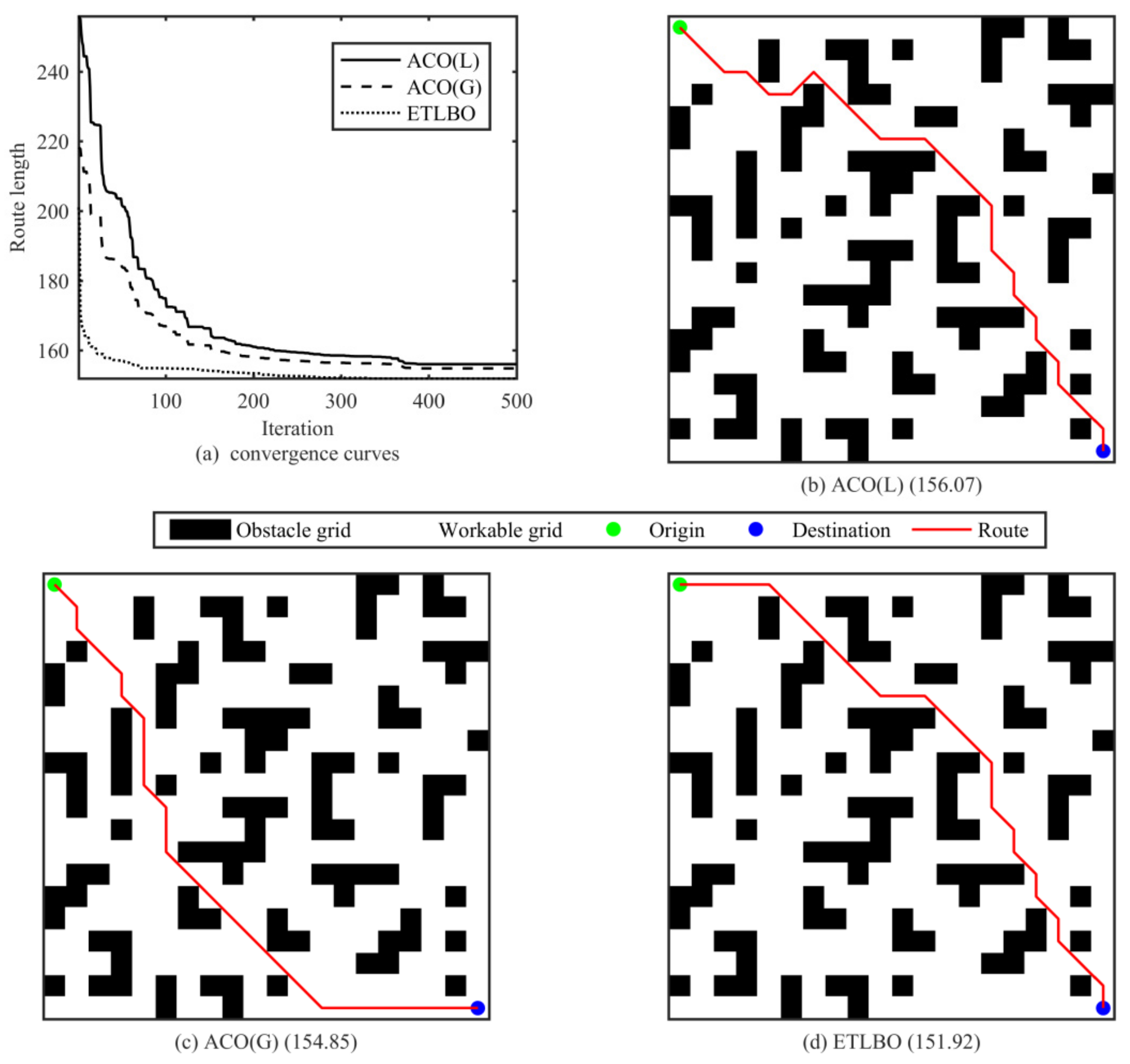
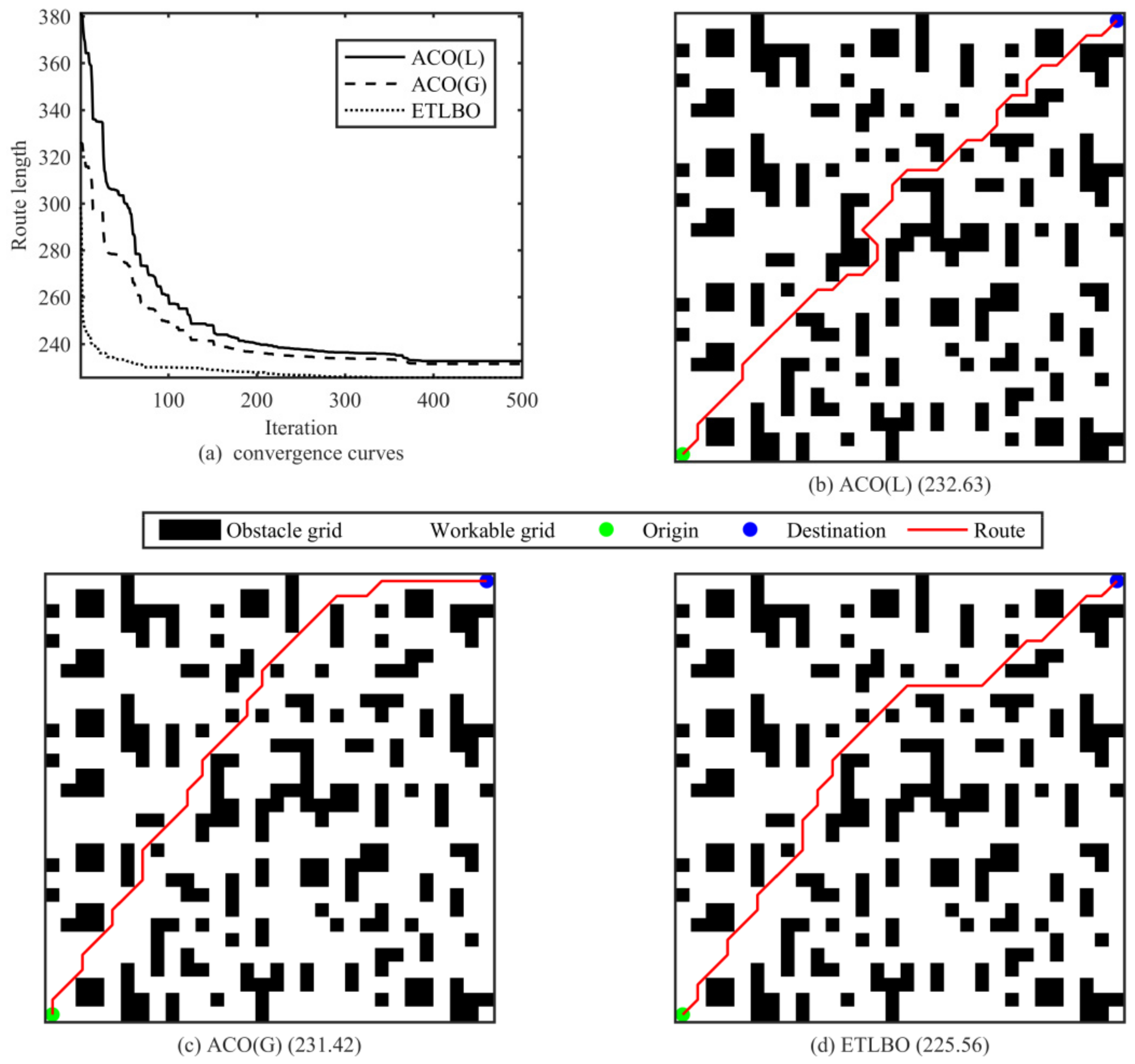
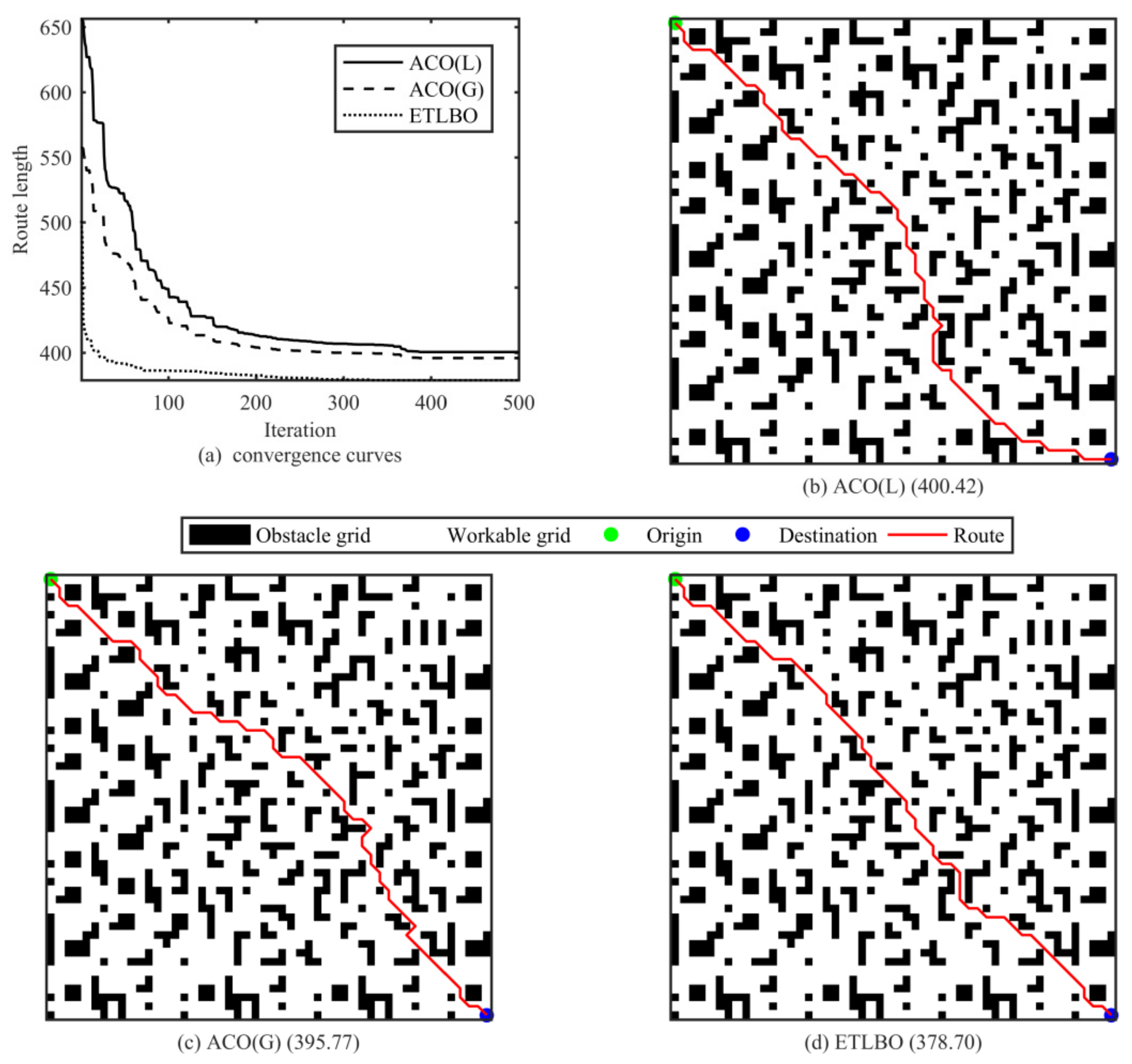
The best routes of information of different algorithms for all instances are detailed in Figure 6, Figure 7, Figure 8 and Figure 9 in order to vividly state the algorithm performance. In this regard, the best robot path for a candidate algorithm for one instance was described by virtue of a single environment map. Meanwhile, objective values versus the number of iterations are illustrated in each figure by means of convergence curves, which represent the best results among 50 independent trials of each algorithm for the corresponding instance. The following comments can be drawn based on these results.

• For instance 20 × 20, it can be seen from Figure 6 that ETLBO yielded the best solution performance of the three test algorithms, with the best route length of 151.92 (Figure 6d). ACO(G) performed second to ETLBO, with the best route length of 154.85 (Figure 6c). ACO(L) showed the weakest performance in the best route length, with an objective value of 156.07 (Figure 6b);
• For the 30 × 30 instance, ETLBO obtained more accurate solutions than ACO(L) and ACO(G) in terms of the best route length metric. The objective value of the proposed ETLBO amounted to 225.56 (see Figure 7d), which is superior to 232.63 (given by ACO(L) in Figure 7b) and 231.42 (provided by ACO(G) in Figure 7c);
• Similar conclusions can be drawn from Figure 8 and Figure 9, in which ETLBO yielded the best solution performance. The corresponding objective values for instances 40 × 40 and 50 × 50 were 291.27 (see Figure 8d) and 378.70 (see Figure 9d), respectively. ACO(G) performed second to ETLBO, with metric values of 291.27 (see Figure 8c) and 378.70 (see Figure 9c). ACO(L) ranked at the bottom, with an objective value of 302.99 (see Figure 8b) and 400.42 (see Figure 9b).
• The convergence curves illustrated in four figures (Figure 6a, Figure 7a, Figure 8a and Figure 9a) indicate that the proposed ETLBO not only had a faster convergence in solving all test instances when compared to the state-of-art ACO(L) and ACO(G) but the final convergence accuracy of the proposed approach was better than that of the compared algorithms.

In summary, among 50 independent trials, the proposed ETLBO exceeded other compared algorithms in terms of the best route length metric.

B. 

Statistical comparison

Table 6. Simulation results for MRPP problems.

Instance	Algorithm	Best		Average		Worst
		Length	Deviation (%)	Length	Deviation (%)	Length	Deviation (%)
20 × 20	ACO(L)	156.07	2.73%	160.16	5.42%	163.64	7.71%
	ACO(G)	154.85	1.93%	158.78	4.52%	161.92	6.58%
	ETLBO	151.92	0.00%	156.64	3.10%	160.71	5.78%
30 × 30	ACO(L)	232.63	3.13%	240.06	6.43%	245.56	8.87%
	ACO(G)	231.42	2.60%	238.56	5.76%	244.35	8.33%
	ETLBO	225.56	0.00%	233.78	3.64%	240.21	6.49%
40 × 40	ACO(L)	302.99	4.02%	313.52	7.64%	322.99	10.89%
	ACO(G)	301.27	3.43%	309.56	6.28%	318.85	9.47%
	ETLBO	291.27	0.00%	303.87	4.33%	312.49	7.28%
50 × 50	ACO(L)	400.42	5.73%	412.07	8.81%	421.13	11.20%
	ACO(G)	395.77	4.51%	409.77	8.20%	418.70	10.56%
	ETLBO	378.70	0.00%	398.27	5.17%	410.42	8.37%

collects the simulation results obtained for all considered problem instances and algorithms. The resulting best, worst, and average objective values, as well as the corresponding deviations, were computed according to 50 independent runs. The best values among the three compared algorithms are emphasized in bold, and the following comments can be drawn according to these results.

• In terms of the optimum, ETLBO was able to find the best solutions for all considered problem instances of different problem scales. However, ACO(L) and ACO(G) failed to obtain the best or near-optimal solutions especially for large-scale problem instances. In this regard, the values of the best deviation metric amounted to 5.73% (given by ACO(L)) and 4.51% (given by ACO(G));
• ETLBO yielded the best solution performance when it was applied to address different problem instances in terms of best-, worst-, and average-related metrics. ACO(G) performed second to ETLBO, while ACO(L) showed the weakest solution performance;
• The average metrics versus the problem size indicated that the increasing problem dimensionality raised the optimization difficulty. In this regard, the average deviations of ACO(L), ACO(G), and ETLBO for the 20 × 20 instance were 5.42%, 4.52%, and 3.10%, respectively. For the large-scale instance with a 50 × 50 size, the average deviations amounted to 8.81%, 8.20%, and 5.17%, respectively;
• Despite the diversity of problem instances, it is evident that all generated values from the proposed ETLBO were more acceptable when compared to the two other algorithms compared.

To reveal the statistical significance of the simulation results, the Wilcoxon rank-sum test was utilized to independently compare the ETLBO with the ACO(L) and ACO(G). As stated in the previous subsection, the value of $w_A$ fell in range [1275, 3775] when comparing ETLBO with another robot-path-planning algorithm. The minimal $w_A$ occurred when ETLBO completely outperformed the compared algorithm in all 50 runs, while the maximal $w_A$ was observed in the circumstance that ETLBO underperformed its rival in all executions. The $w_A$ metric and the $p$ values of the Wilcoxon rank-sum test associated with each compared algorithm were calculated and presented in

Table 7. Wilcoxon rank-sum test for MRPP problems.

Instance	ACO(L)			ACO(G)
	${\mathit{w}}_{\mathit{E}\mathit{T}\mathit{L}\mathit{B}\mathit{O}}$	$\mathit{p}$	Win	${\mathit{w}}_{\mathit{E}\mathit{T}\mathit{L}\mathit{B}\mathit{O}}$	$\mathit{p}$	Win
20 × 20	1590	5.75 × 10−11	√	1631	3.56 × 10−10	√
30 × 30	1399	4.16 × 10−15	√	1575	2.89 × 10−11	√
40 × 40	1300	1.52 × 10−17	√	1438	3.35 × 10−14	√
50 × 50	1275	3.42 × 10−18	√	1342	1.74 × 10−16	√

, where mark “√” represents a win for ETLBO over its rival.

In respect to the comparison between ETLBO and ACO(L), the following comments can be made:

• For the 50 × 50 instance, the associated rank sum of ETLBO was 1275, and the resulting $p$ value was very close to zero. As is stated in previous subsections, the significance level was fixed at 0.05 for this study. Therefore, it can be deduced that ETLBO dominates the ACO(L) in all executions when they are adopted to this instance.
• For the instances 20 × 20, 30 × 30, and 40 × 40, the rank sum of ETLBO lay between the maximum and minimum rank threshold values, indicating that ETLBO and ACO(L) produced a mixed ranking. Nonetheless, the associated $p$ values were less than the predefined significance level. In other words, ETLBO performs equally or even better when compared to ACO(L).
• Despite the increasing problem dimensionality raising the optimization difficulty, the resulting $p$ values decreased with the enlargement of the problem scale. Thus, it can be deduced that ETLBO is more competitive than ACO(L) for a real-world-scale problem.

A similar comparison between ETLBO and ACO(G) was conducted and illustrated. In summary, the proposed ETLBO outperforms the compared algorithms in a statistical manner and provides consistent and more accurate solutions for MRPP problems.

6. Conclusions

This research proposes a so-called ETLBO algorithm to realize an efficient path planning for a mobile robot. Four strategies are introduced to accelerate the basic TLBO algorithm and optimize the final path. Firstly, a divide-and-conquer design coupled with the Dijkstra method is developed to realize the problem transformation so as to pave the way for the algorithm deployment. Then, the interpolation method is utilized to smooth the traveling route as well as to reduce the problem dimensionality. Thirdly, the algorithm initialization process is modified by an opposition-based learning strategy. Finally, a hybrid individual update method is prosed to strike a balance between exploitation and exploration.

Simulation experiments are designed to validate the proposed algorithm. In terms of benchmark function problems, the proposed ETLBO performs better than the compared algorithms in a statistical manner and obtains consistent and more accurate solutions for most optimization function problems. With respect to MRPP problems, ETLBO outperforms some state-of-are algorithms in both optimality and efficiency, and thus can be implemented on the real-world robot for path planning.

Since the local optimal path planning in current algorithm is solved by the Dijkstra method, it is important to modify the existing divide-and-conquer design in future research work to reduce the computation burden when faced with more complicated practical problems. In addition, the proposed methodology can be adjusted and adapted to the dynamic environment in which certain real-time factors are seriously considered.

References

1. Friudenberg, P.; Koziol, S. Mobile robot rendezvous using potential fields combined with parallel navigation. IEEE Access 2018, 6, 16948–16957. [Google Scholar] [CrossRef]
2. Contreras-Cruz, M.A.; Ayala-Ramirez, V.; Hernandez-Belmonte, U.H. Mobile robot path planning using artificial bee colony and evolutionary programming. Appl. Soft Comput. 2015, 30, 319–328. [Google Scholar] [CrossRef]
3. Binh, N.T.; Tung, N.A.; Nam, D.P.; Quang, N.H. An adaptive backstepping trajectory tracking control of a tractor trailer wheeled mobile robot. Int. J. Control Autom. Syst. 2019, 17, 465–473. [Google Scholar] [CrossRef]
4. Kellalib, B.; Achour, N.; Coelen, V.; Nemra, A. Towards simultaneous localization and mapping tolerant to sensors and software faults: Application to omnidirectional mobile robot. Proc. Inst. Mech. Eng. Part I J. Syst. Control Eng. 2020, 235, 269–288. [Google Scholar] [CrossRef]
5. Ab Wahab, M.N.; Nefti-Meziani, S.; Atyabi, A. A comparative review on mobile robot path planning: Classical or meta-heuristic methods? Annu. Rev. Control 2020, 50, 233–252. [Google Scholar] [CrossRef]
6. Orozco-Rosas, U.; Montiel, O.; Sepúlveda, R. Mobile robot path planning using membrane evolutionary artificial potential field. Appl. Soft Comput. 2019, 77, 236–251. [Google Scholar] [CrossRef]
7. Liu, J.; Yang, J.; Liu, H.; Tian, X.; Gao, M. An improved ant colony algorithm for robot path planning. Soft Comput. 2017, 21, 5829–5839. [Google Scholar] [CrossRef]
8. Akka, K.; Khaber, F. Mobile robot path planning using an improved ant colony optimization. Int. Ournal Adv. Robot. Syst. 2018, 15, 1729881418774673. [Google Scholar] [CrossRef]
9. Nazarahari, M.; Khanmirza, E.; Doostie, S. Multi-objective multi-robot path planning in continuous environment using an enhanced genetic algorithm. Expert Syst. Appl. 2019, 115, 106–120. [Google Scholar] [CrossRef]
10. Wang, G.; Zhou, J. Dynamic robot path planning system using neural network. J. Intell. Fuzzy Syst. 2021, 40, 3055–3063. [Google Scholar] [CrossRef]
11. Zhao, J.; Cheng, D.; Hao, C. An improved ant colony algorithm for solving the path planning problem of the omnidirectional mobile vehicle. Math. Probl. Eng. 2016, 2016, 7672839. [Google Scholar] [CrossRef]
12. Wu, X.; Wei, G.; Song, Y.; Huang, X. Improved ACO-based path planning with rollback and death strategies. Syst. Sci. Control Eng. 2018, 6, 102–107. [Google Scholar] [CrossRef]
13. Wang, H.; Guo, F.; Yao, H.; He, S.; Xu, X. Collision Avoidance Planning Method of USV Based on Improved Ant Colony Optimization Algorithm. IEEE Access 2019, 7, 52964–52975. [Google Scholar] [CrossRef]
14. Yue, L.; Chen, H. Unmanned vehicle path planning using a novel ant colony algorithm. EURASIP J. Wirel. Commun. Netw. 2019, 2019, 136. [Google Scholar] [CrossRef]
15. Chen, G.; Liu, J. Mobile Robot Path Planning Using Ant Colony Algorithm and Improved Potential Field Method. Comput. Intell. Neurosci. 2019, 2019, 1932812. [Google Scholar] [CrossRef]
16. Dai, X.; Long, S.; Zhang, Z.; Gong, D. Mobile Robot Path Planning Based on Ant Colony Algorithm with A Heuristic Method. Front. Neurorobotics 2019, 13, 15. [Google Scholar] [CrossRef]
17. Luo, Q.; Wang, H.; Zheng, Y.; He, J. Research on path planning of mobile robot based on improved ant colony algorithm. Neural Comput. Appl. 2019, 32, 1555–1566. [Google Scholar] [CrossRef]
18. Miao, C.; Chen, G.; Yan, C.; Wu, Y. Path planning optimization of indoor mobile robot based on adaptive ant colony algorithm. Comput. Ind. Eng. 2021, 156, 107230. [Google Scholar] [CrossRef]
19. Rao, R.V.; Savsani, V.; Vakharia, D.P. Teaching–learning-based optimization: A novel method for constrained mechanical design optimization problems. Comput.-Aided Des. 2011, 43, 303–315. [Google Scholar] [CrossRef]
20. Rao, R.V.; Patel, V. An improved teaching-learning-based optimization algorithm for solving unconstrained optimization problems. Sci. Iran. 2013, 20, 710–720. [Google Scholar] [CrossRef] [Green Version]
21. Camp, C.V.; Farshchin, M. Design of space trusses using modified teaching–learning based optimization. Eng. Struct. 2014, 62, 87–97. [Google Scholar] [CrossRef]
22. Rao, R.V. Teaching-learning-based optimization algorithm. Teaching Learning Based Optimization Algorithm; Springer: Cham, Switzerland, 2016; pp. 9–39. [Google Scholar]
23. Zou, F.; Chen, D.; Xu, Q. A survey of teaching–learning-based optimization. Neurocomputing 2019, 335, 366–383. [Google Scholar] [CrossRef]
24. Das, S.; Suganthan, P.N. Differential evolution: A survey of the state-of-the-art. IEEE Trans. Evol. Comput. 2010, 15, 4–31. [Google Scholar] [CrossRef]
25. Diwan, S.P.; Deshpande, S.S. Fast Nonlinear Model Predictive Controller using Parallel PSO based on Divide and Conquer Approach. Int. J. Control 2022, 1–10. [Google Scholar] [CrossRef]
26. Lin, D.; Shen, B.; Liu, Y.; Alsaadi, F.E.; Alsaedi, A. Genetic algorithm-based compliant robot path planning: An improved Bi-RRT-based initialization method. Assem. Autom. 2017, 37, 261–270. [Google Scholar] [CrossRef]
27. Mahdavi, S.; Rahnamayan, S.; Deb, K. Opposition based learning: A literature review. Swarm Evol. Comput. 2018, 39, 1–23. [Google Scholar] [CrossRef]
28. Xu, L.; Cao, X.; Du, W.; Li, Y. Cooperative path planning optimization for multiple UAVs with communication constraints. Knowl.-Based Syst. 2023, 260, 110164. [Google Scholar] [CrossRef]
29. Alorf, A. A survey of recently developed metaheuristics and their comparative analysis. Eng. Appl. Artif. Intell. 2023, 117, 105622. [Google Scholar] [CrossRef]
30. Hashim, F.A.; Mostafa, R.R.; Hussien, A.G.; Mirjalili, S.; Sallam, K.M. Fick’s Law Algorithm: A physical law-based algorithm for numerical optimization. Knowl.-Based Syst. 2023, 260, 110146. [Google Scholar] [CrossRef]
31. Shukla, A.K.; Singh, P.; Vardhan, M. An adaptive inertia weight teaching-learning-based optimization algorithm and its applications. Appl. Math. Model. 2020, 77, 309–326. [Google Scholar] [CrossRef]
32. Gao, W.; Tang, Q.; Ye, B.; Yang, Y.; Yao, J. An enhanced heuristic ant colony optimization for mobile robot path planning. Soft Comput. 2020, 24, 6139–6150. [Google Scholar] [CrossRef]
33. Yin, L.; Li, X.; Lu, C.; Gao, L. Energy-efficient scheduling problem using an effective hybrid multi-objective evolutionary algorithm. Sustainability 2016, 8, 1268. [Google Scholar] [CrossRef] [Green Version]
Figure 1. Grid environment map.
Applsci 13 02291 g001
Figure 2. Possible movements of the robot.
Applsci 13 02291 g002
Figure 3. Divide-and-conquer design for MRPP.
Applsci 13 02291 g003
Figure 4. Schematic diagram of interpolation method.
Applsci 13 02291 g004
Figure 5. Proposed ETLBO for the MRPP.
Applsci 13 02291 g005
Figure 6. Best solution information of instance 20 × 20.
Applsci 13 02291 g006
Figure 7. Best solution information of instance 30 × 30.
Applsci 13 02291 g007
Figure 8. Best solution information of instance 40 × 40.
Applsci 13 02291 g008
Figure 9. Best solution information of instance 50 × 50.
Applsci 13 02291 g009