Abstract
Safety and comfort are the two major requirements for the successful implementation of self-driving cars, which are anticipated to constitute the future generation of transportation. To create safe and effective self-driving car trajectories, a novel behavioral decision model is developed. First, a risk field model for driving activities based on vehicle kinematics and Eulerian solenoids is constructed. From there, the principle of least action is applied to produce the best trajectory points. Finally, nine typical unit scenarios are simulated by matlab’s driving scenario designer to verify the feasibility of the decision-making algorithm. This study illustrates how an unified operational risk field can efficiently increase intersection passing efficiency while ensuring safety, utilizing the principle of least action. The experimental results show that in the scenario of unprotected left turn and more than 5 vehicles in the intersection, the decision-making model improves the pass rate by 23% compared with the TTI (Time To Intersection) threshold method.
1. Introduction
The commercialization of automated driving is transforming how people travel. Thus, it is crucial that the trajectory of self-driving cars be developed in a fashion that considers passenger comfort and movement efficiency while maintaining safety. In the United States, Waymo will launch its first driverless taxi service in the Phoenix, Arizona area in December 2021, however the service will still require remote human supervision [1]. In Japan, Honda was authorized to produce Level 3 autonomous vehicles (AVs) in March 2021 and offered Level 4 services for the 2020 Tokyo Olympics [2,3]. Pony.ai’s commercial autonomous driving operations in China have covered 85,476 km, and test operations have begun in a number of significant Chinese cities, including Beijing and Shenzhen [4]. While commercial use of autonomous driving is being deployed progressively, issues are also coming to light. Even though autonomous driving systems have the greatest right of way on the road, they are too “considerate” drivers and always give way to approaching vehicles. Additionally, in complicated urban driving situations, autonomous driving systems are frequently overloaded and need a human driver’s assistance [5].
The complexity of the processing needed for self-driving automobiles, as depicted in Figure 1, is sharply increased by the presence of pedestrians and non-motorized vehicles on metropolitan highways. How do self-driving cars navigate busy crossroads with plenty of traffic and risky side streets? Making rational decisions using predetermined decision models in such situations is difficult for computer processing systems. On the other hand, despite the fact that they may not be doing it themselves, pedestrians and non-motorized vehicles frequently have the greatest right of way in these situations due to respect for and compliance with traffic laws. The interaction between right-of-way, regulations, and the trajectory of the AV movement is also brought up in this, which is crucial information for the designers of autonomous driving systems. Additionally, as seen in Figure 1, the self-driving vehicle might need to exit the intersection earlier to allow adequate room for the black car to pass through. This is necessary for the self-driving vehicle and the human-driven vehicle to collaborate with one another.
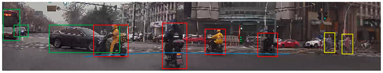
Figure 1.
Typical urban traffic complex scenario where the host vehicle needs to interact with different types of traffic participants.
To address these issues, we propose constructing a unified driving operation risk field (UDORF) model using the Eulerian spiral and the vehicle dynamics model as references. Based on this model, we suggest assigning numerous weights to the various traffic participant types that were identified, and then generating the ideal trajectory using the principle of minimum action. Figure 2 depicts the proposed method’s flowchart. We gather data on the category and status of traffic participants, lane lines, and traffic signals via Mobileye module, and calibrate the distance data collected by Mobileye using 32-line LIDAR for use in environment perception and scene generation. With the use of this knowledge, the self-vehicle detects and comprehends its surroundings and determines the best place to move to next. We use MATLAB Driving Scenario Designer application for simulation scenario construction and algorithm simulation.
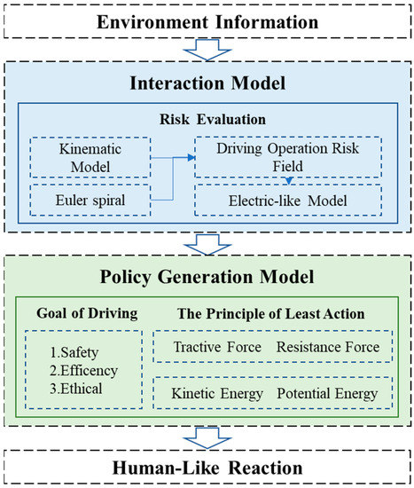
Figure 2.
Overview of the decision model for AVs.
The primary modeling entities for the current major research mostly pertain to cars because they are the primary traffic players in the vehicle driving scenario. By using scene identification and target tracking algorithms in a static environment, AVs’ perception abilities have advanced significantly in software. Additionally, the capacity of AVs’ perception systems and trajectory creation will be strongly impacted by the ability to precisely predict the motion trajectories of nearby traffic participants using tools like kinematic dynamics models or Gaussian noise simulations. As a result, the problem of environmental risk assessment and local path planning for smart vehicles is receiving increasing attention from the scientific community. The primary modeling entities for the current major research mostly pertain to cars because they are the primary traffic players in the vehicle driving scenario. Existing local path planning methodologies can be divided into three primary groups: those that use driver intent prediction, driver physics models, and social interaction. For example, ref. [6] constructs costly maps and obtains the least costly local path by the RRT (Rapidly-exploring Random Trees) method. Whereas [7] reduces the risk during driving by computing trajectories that maximize visibility, the problem of violating certain rules often arises. To avoid such problems, ref. [8] proposed a method to synthesize only the motions that violate the lowest priority rules in the shortest time possible, and although it seems to work, the integrated challenge of autonomous driving makes it challenging in non-deterministic systems and environments. In addition, In [9], the authors use two optimal search algorithms, A* and D*, to find the globally optimal path that connects the initial position of each cell to the target position. The researchers in [10] used the tentacle method to generate a set of tentacles as feasible trajectories on a self-centred occupancy grid around a running vehicle.
Among these, the artificial potential field-based approach, in the area of autonomous cars, includes risk assessment techniques based on vehicle physics models and driver intent-based predictions, enabling efficient risk modeling of the immediate environment surrounding the vehicle. Due to its ability to easily visualize the static environment information surrounding a robot, the traditional artificial potential field method has historically been one of the most well-liked research directions for robot path planning algorithms. However, while the algorithm has a workable solution in time, it has the disadvantage of exponentially increasing in spatial complexity as the spatial extent increases. Additionally, it is not guaranteed to produce globally optimal outcomes due to its weak capacity to service local minimum traps. To address this issue, numerous researchers have developed techniques including shape representation approaches [11] and simulated annealing algorithms [12]. Ref. [13] constructed a discrete artificial potential field, which was customised and tuned to achieve a fast and efficient solver that could operate in near real-time in complex environments. A unified model of “driving risk field” was constructed for the closed-loop system of human-vehicle-road in order to expose the mechanism of human-vehicle-road interaction, the influence law of each element of traffic on driving safety, and to anticipate the dynamic changing trend of driving risk [14]. The model is based on field theory and introduces the new concept of “driving risk field”, which includes “kinetic field” determined by motor vehicles, non-motorized vehicles, and other moving objects on the road, “potential field” produced by road environment elements, and “behavior field” determined by individual characteristics of drivers. Based on the findings of the research, ref. [15] proposed a spring-like model risk assessment method to improve the artificial potential field. When combined with the minimum action method, the action generation problem was subsequently reduced to an optimization problem, leading to improved experimental outcomes at the intersection. However, because the spring-like model created by the model is unable to properly separate some unimportant aspects, it is challenging to guarantee the smooth passage of vehicles in complicated road conditions. This work provides a unified driving operation risk field model and enhances the artificial potential field creation method to circumvent such issues. The model employs The Euler spiral to determine the predicted driving arrival range of vehicles and influences the host vehicle based on a single criterion (maximum overlap area), guaranteeing that it does not slip into a local optimum in complex circumstances.
2. Materials and Methods
2.1. Driving Operation Risk Field
As was previously indicated, the majority of the hazards that the vehicle encounters come from factors that are dangerous up front and that also fall within the driver’s operable range while driving on the road. To define this range, we propose a driving operation risk field boundary, as illustrated in Figure 3.
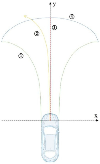
Figure 3.
Driving operation risk field boundary.
The most effective technique a driver can do to avoid the front’s largest hazard is emergency braking, and taking into account the self-braking vehicle’s requirements, the following (Time To Stop) based on speed is implied:
where is the ego vehicle’s speed at time , an is the braking deceleration applied by the driving system at time , and is the amount of environmental road friction present where the vehicle is located because both the environment and the road conditions have an impact on the vehicle’s braking performance [16].
Additionally, as most drivers use adaptive maneuvers to protect the security and comfort of their own vehicles, the autonomous driving system’s estimation of the threat level should take this into account. In order to satisfy the braking requirements for collision avoidance, we take into consideration three deceleration thresholds in this study and build the driving operation risk field based on them. The three recently established deceleration thresholds are: (1) emergency braking, (2) moderate braking to slow, and (3) gentle braking for comfort while driving [17]. The following are the deceleration thresholds that correspond to them:
Therefore, the corresponding to the three thresholds is defined as:
For the described risk field, a simplified two-wheel model of the vehicle is used in this paper. The risk field of driving operation is delimited by four curves, as depicted in Figure 3, namely ① Euler spiral, ② normal driving trajectory line, ③ braking trajectory line, and curve ④ which fits the extreme points of ① and ③.
For curve ①, which is characterized by a curve whose radius of curvature r decreases with the length of the curve s and describes the turning maneuver of the vehicle in the limit situation (when the centrifugal acceleration and the vehicle deceleration reach a maximum combination), we introduce the Eulerian spiral [18], which is defined as:
where , are the distance traveled and the farthest distance measured along the spiral curve from the initial position, respectively, and the constant is referred to as the flatness of the gyrus line or the isospin parameter, expressed as:
where is the radius of rotation of the gyrus line at . Expressing the distance s traveled by the vehicle at moment with the radius of rotation as a kinematic parameter, we obtain:
where denotes the initial velocity of the vehicle, denotes the centripetal acceleration, and denotes the longitudinal backward deceleration of the vehicle in the AV coordinate system. Ultimately, curve ① can be expressed as
where is the vehicle width, is the time required for the vehicle speed to become 0, denotes the initial steering wheel turning angle of the vehicle, and the constant denotes the weights of the two Eulerian spirals to the left and right of the specialized vehicle.
For curve ②, which is used to contrast with the Eulerian trajectory curve, describes the steering trajectory during routine vehicle operation without reacting to an emergency scenario. The curve behaves as a circle, specified by the following equation, because it is defined by the highest centrifugal acceleration, , and moves at the original speed.
For curve ③, the trajectory for the vehicle to maintain the initial steering wheel angle while reaching the maximum deceleration. This paper is divided into two cases for discussion.
(1) When the vehicle steering angle is zero, represented by a straight line, defined by a simple parametric equation.
(2) When the vehicle steering angle is non-zero, similar to curve 2, but since the velocity is not constant, the travel trajectory curve can be obtained from the simplified two-degree-of-freedom steering model as follows.
where is the vehicle length, is a constant, and v is the velocity component along the -axis in the body coordinate system.
For curve ④, it is the fitted circular curve of curve ① and curve ③ out at the end point. The range bounded by curves ①, ③ and ④ indicates the braking range of the vehicle in the limit avoidance condition, into which the driving operation can no longer be used to avoid a collision. The relaxation of conditions, for example by reducing the expected braking acceleration, mimics the risk field that human drivers are concerned with during driving. As a comparison, curve ② allows for a wider risk field than can be achieved by normal driving, thus leaving sufficient safety redundancy.
2.2. Electric-like Field Model
To interact with other traffic players and their operational risk fields, we presume in this model that the self-vehicle carries electric charge. The overlapping region will increase the charge q and accrue potential energy with the area of the region whenever other traffic participants or their risk fields enter the self-vehicle risk field. Depending on the severity, the cost borne by other traffic participants and their operational risk fields per unit area varies in size. As a result, it can be said as follows.
where represents the various areas where the same target’s operational risk field and the self-vehicle risk field overlap, where . is the area of the various risk field regions occupied by the overlapping regions, and is the risk weight of the risk field regions. is usually taken as 1. Assuming equal distribution of the charges in the electric field-like model, we can compare the overlapping regions to point charges at their centroid locations. The centroid position can be expressed as
where , are the horizontal and vertical coordinates in the region under the self-carriage coordinate system.
is the separation between the center of the overlapping region and the vehicle’s center of gravity, and the resulting Coulomb force is defined as
The computational basis of the electric field-like model is shown in Figure 4. As shown in this diagram, the green point is the centre of the overlap of the green vehicle in the risk field of the blue vehicle driving operation and influences the direction of the repulsive force on the blue vehicle . This overlap influences the magnitude of the repulsive force. Similarly, the effect of the orange vehicle on the blue vehicle is derived in this way. It demonstrates how other factors, such as the two vehicles’ speeds and heading angles, can also have an impact on how severe an encounter between two moving objects is. It is important to note that the red area in the diagram represents the range that the self-vehicle can travel in the case of an emergency. As a result, different entities are not permitted to enter this area because doing so would result in an accident. Additionally, if this range overlaps with another area, the operational risk field of other traffic participants would also be given a high risk weight.
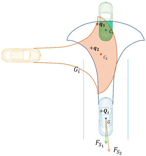
Figure 4.
Electric field-like model.
According to [12], accidents are anomalous transfers in the context of energy transfer theory. According to [19], the relationship between the various activities suggested determines the equivalent force caused by the self-vehicle when it is moving at a constant speed. Then, the self-vehicle ’s force with the virtual point charge is provided by
where and stand for the self-vehicle ’s mass and speed, respectively. So, it is established that
From this, we can obtain
Given that k and have constant values, must also be constant when is constant. The above equation demonstrates that when the self-vehicle maintains a constant speed, an increase in results in an increase in the risk to the self-vehicle, which must result in an increase in the distance r between the self-vehicle and the virtual point charge; conversely, a decrease in results in a reduction in the risk to the self-vehicle, and the self-vehicle can shorten the distance r between the virtual point.
The self-vehicle will experience inertial forces, which can be described as follows, when it travels at a constant rate of acceleration and deceleration.
In summary, in this study we apply the operational risk field and its resulting electric field-like forces and potentials to describe the interaction between vehicles.
Therefore, combining the above equation and (16) equation, the Coulomb force applied to the self-car can be expressed as
2.3. Decision-Making Model
2.3.1. Decision-Making Goals
In various traffic situations, drivers have varied driving objectives. For instance, in high-speed road conditions, drivers must keep a steady speed to conserve fuel and time. In urban road environments, drivers must be mindful of non-motorized vehicles and pedestrians around to reduce the occurrence of ghost probes. Additionally, there are certain standards to guarantee the comfort of the passengers. For example, careful driving is necessary in traffic jams to prevent frequent and excessive acceleration and deceleration.
As a result, “safety” and “efficiency” were selected as the drivers’ key aims to take into account while driving, with “orderliness” selected as a secondary priority. Among these, safety entails avoiding collisions and using defensive driving, high efficiency entails making decisions quickly and with as little change as possible, and orderliness entails adhering to traffic regulations. This additional objective was established because, in some severe emergency scenarios, the system will prioritize safety over traffic compliance.
We introduce the principle of least action and the decision model based on it in the following subsections.
2.3.2. The Principle of Least Action
The car can be thought of as an energy conservation mechanism during the ideal driving process, which is to say, disregarding road friction. The attraction potential energy G exists to provide an attractive force that prompts the vehicle to travel to the target point. As this potential energy G was released, the vehicle’s kinetic energy gradually increased, where the release and absorption of energy were in accordance with the law of energy conservation. The concept of least action has been extensively used in the study of electromagnetic fields, gravitational fields, and classical dielectric mechanics. It is a fundamental variational principle for particles and continuous systems. The principle is first applied by [15] in the field of trajectory generation for autonomous driving. In [15], by imagining all possible trajectories that the system can imagine, computing the actions (functions of the trajectory) for each trajectory, finding the true dynamic trajectory of the system between the initial and final configurations in a specified time, and choosing an action that makes the actions partially stationary (traditionally called “least”), then the true trajectories are those with the fewest actions. If we use 𝑆 to represent the action, the principle can be expressed as .
The primary objective of automated driving systems is to maximize gains and minimize losses, similar to the primary objective of human driving. Whereas gains stand in for effectiveness and safety, and losses for improper driving and violations. The minimum action can be described as follows if we use the kinetic energy of the vehicle along with the force and potential energy produced by interaction with other traffic participants as the safety criterion and the trip time as the efficiency requirement. The primary objective of automated driving systems is to maximize gains and minimize losses, similar to the primary objective of human driving. Whereas gains stand in for effectiveness and safety, and losses for improper driving and violations. The minimum action can be described as follows if we use the kinetic energy of the vehicle along with the force and potential energy produced by interaction with other traffic participants as the safety criterion and the trip time as the efficiency requirement.
where and stand for the vehicle’s kinetic and potential energy, respectively, and L is the Lagrangian quantity. Ref. [12] defines an accident as an abnormal transfer of a vehicle’s potential energy, which is followed by the vehicle’s elastic and plastic deformation. As a result, the vehicle’s kinetic energy can be thought of as its own risk, and the process of accelerating the vehicle from a stop to a particular speed can be thought of as the accumulation of the vehicle’s risk. The relationship between the vehicle and the goal point as well as the relationship between the vehicle and the surrounding traffic environment are both included in the potential energy . As an illustration, Figure 4 illustrates how, in the adjacent lane, the potential energy associated with the target point always decreases while the kinetic energy increases. In contrast, the potential energy associated with the vehicle and the surrounding traffic environment increases and then decreases as the risk field state changes as a result of oncoming traffic coming from the opposite direction, while the kinetic energy appropriately releases the energy before absorbing it. Additionally, the times and , which in this calculation stand in for the start and finish times, respectively, signify the efficiency of the passage as well as the accumulation of risk. Therefore, the safer and more effective the driving procedure, the less the value of .
2.3.3. Decision-Making Model
As seen in Figure 5, the gravitational force that the target point exerts on the AV serves as its driving force. The acceleration brought on by the pseudo-gravitational force will be constrained by the expected speed with the limited speed in order to prevent unrestricted acceleration in special circumstances. It is capable of defining the driving force as:
where denotes the mass of vehicle i, and denotes the acceleration due to class gravity. We define as
where is a constant (here we take = 0.2), is the driver’s desired velocity, is the limiting velocity, and is denoted as the gravitational acceleration.
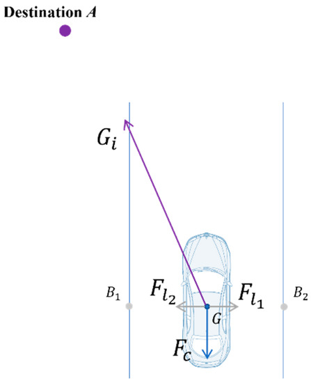
Figure 5.
Schematic diagram of the effect of basic forces.
In addition, traffic rules also exert a force on the driver to keep the speed within a reasonable range: the driving force will drive the vehicle to accelerate when the self vehicle speed is less than the required minimum speed of the current road, and the binding force will constrain the vehicle to slow down when the self vehicle speed is greater than the required maximum speed of the current road. We define the traffic rule binding force as.
Also, to ensure that AVs do not change lanes unnecessarily and maintain their current lane at intersections or other non-lane change scenarios, we define lane repulsion as follows.
where denotes the road type (where we take dot line for and solid line for with intersection lane line ), denotes the distance between the lane line and the vehicle center point on both sides and is a constant (take ).
Although UDORF has simplified the in-junction scenario significantly, further extraction of key information is still needed to shorten the evaluation process. Figure 5 illustrates that natural driving scenarios can be obtained from the following equations.
where denotes the attractive force acting on vehicle i and denotes the hindering force, which includes the traffic rule binding force , the lane repulsion force and the electric field-like force .
Therefore, the driving action of the vehicle can be obtained by the following equation.
The same is true for the cost function of the multiple objective decision model. The cost function takes into account safety and efficiency to optimize the driving decision process. In addition, we will illustrate this cost function in the next section using specific examples.
3. Results
To verify the efficacy of the suggested cost function S, we conduct some simulation experiments in this section. As shown in Figure 6, where the blue vehicle (vehicle i) represents the self-vehicle and the brown vehicle (vehicle j) represents the leading vehicle in the traffic flow, we design an unprotected intersection to verify the effectiveness of the proposed behavioral decision model approach. This addresses the current challenge for self-driving cars to pass in complex urban intersection scenarios. We streamline the traffic flow to the leading vehicle j in the analysis to make it simpler to comprehend.
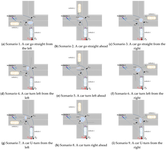
Figure 6.
Different scenarios of left-turn at an unprotected intersection.
When self-vehicle i approaches the intersection along the trajectory line obtained from global path planning and turns left, it will encounter one of the following nine unit scenarios or a combination thereof: (a) vehicle j approaches the intersection from the left; (b) vehicle j approaches the intersection from the right; (c) vehicle j approaches the intersection from the front; (d) vehicle j makes a left turn on the left side of the intersection; (e) vehicle j makes a left turn in front of the intersection; (f) vehicle j makes a left turn on the right side of the intersection; (g) vehicle j makes a right turn on the left side of the intersection; (h) vehicle j makes a right turn in the front of the intersection; (k) vehicle j makes a right turn on the right side of the intersection. The objective of the AV i is to turn left from the current lane into the left side of the intersection according to the pre-planned global route without crossing the invisible intersection lane line and without colliding with the surrounding traffic participants.
3.1. Decision Making on Unit Scenarios
The self-driving automobile is impacted by the following four primary factors, as previously mentioned: attraction force , binding force on traffic rules , lane repulsion force , and electric field-like force . These forces are explained in Figure 6. Since each model used in this study is built using the self-vehicle coordinate system, the cost function of the decision model is given by the equation below.
There is a path along which an AV can modify its behaviors the fewest number of times, in accordance with the principle of least action. This route here corresponds to the safest and most effective driving technique. As a result, this approach has theoretically zero S variation. It is described by the equation below.
The lagrangian quantities are transformed to a self-carrying Cartesian coordinate system under to make computations simpler.
where is the angle between the potential field force and the binding force , , and is the angle between the driving force and the binding force , . The counterclockwise direction is set as the positive direction.
Bringing the above equation into the Eulerian Lagrange equation, it is obtained that
According to the aforementioned equation, the vehicle always satisfies the mechanical balance in both longitudinal and lateral directions when traveling along the ideal path indicated above. In this scenario, the aforementioned equation enables the calculation of the vehicle’s minimum movement and the associated amount of transverse-longitudinal control at various times.
3.2. Simulation Results
The MATLAB Driving Scenario Designer Toolbox created the driving simulation scenario for this investigation. In the tool box scenario editor, we first add the road model and apply a binding force to the target vehicle by setting the constants as described above. After that, we add sensors and adapt them to sense where the lane lines on either side are closest to the vehicle; artificially set target points and add functions to make them attractive to the vehicle; add road friction and set friction coefficients. In addition, during the actual simulation, the area and center point of the overlap range of the risk field of the driving operation of the target vehicle and other vehicles, calculated by the function, with the current coordinate point of the center of gravity of the target vehicle, provides the repulsive force to the target vehicle. For the purpose of algorithm verification, the environment automatically delivers all vehicle status data, including absolute/relative position, absolute/relative speed, and heading angle.
The algorithm for the behavioral decision model is displayed in Algorithm 1. The primary vehicle identifies the surrounding vehicles’ states. An interaction model built based on the risk field is then used to determine the size and direction of the potential field forces on the main vehicle. In order for the car to cross the intersection smoothly, the algorithm determines the lowest amount of horizontal and vertical control.
| Algorithm 1 Decision making based on artificial potential field | |
| Input | t |
| Output | |
| 1 | Initialize ←3.5, S←0, T←0, U ← 0 |
| 2 | Get the terminal point |
| 3 | Define the attractive force: |
| 4 | Define the constraint resistance force: |
| 5 | Define the lane marker force: |
| 6 | while True do |
| 7 | Get the absolute states of ego vehicle (), |
| 8 | if |
| 9 | Break |
| 10 | end if |
| 11 | Get the relative states of surrounding vehicles (), j = 1,2,… |
| 12 | Construct the ego vehicle’s operation risk field and other vehicles’ driver risk field respectively |
| 13 | Calculate the centroid and area of the interactive region |
| 14 | Calculate the potential energy and force obtained by the vehicle through the risk field |
| 15 | Define the kinetic energy of the vehicle: |
| 16 | Calculate the cost function of the minimum action principle |
| 17 | Get the acceleration and heading angle of the ego vehicle by calculating the constraints of and |
| 18 | end while |
We initially presummated that the cars in the simulation tests, aside from the target vehicle I, were moving like a human. The beginning conditions of vehicle speed from 7 to 24 m/s and vehicle distance from 15 to 50 m were used to replicate each of the nine aforementioned scenarios 100 times.
We evaluate the proposed method from three perspectives, namely its adaptability to the scenario, its stability and its effectiveness. We generated mean S-value plots from the experimental results to reflect the sensitivity of the method to each parameter in the scenario. Transverse and longitudinal velocity and heading angle plots were generated to reflect the stability of the method’s decisions, which is ensure the comfort of the passengers. Pass-by plots were generated to compare with the TTI method to reflect the effectiveness of the method in the scenario. Figure 7 illustrates the average S-values generated in nine typical scenarios for driving operational risk fields at different distances and speeds. This S-value represents the corresponding magnitude of risk that the AV responds to. We represent the reaction mechanism of the ego vehicle in this scenario by the lateral and longitudinal speed and heading angle of the ego car. Figure 8 shows a typical curve of the speed and heading angle of the vehicle when other agents enter from the left side of the intersection. It can be seen that under different initial conditions, the vehicle’s lateral speed always maintains a smooth increase, which means that in the task of turning left at the intersection, the response mechanism provides a long-term effect and keeps the whole process of turning coherent. In addition, the host vehicle frequently keeps the vehicle in a relatively safe position and coasts forward in terms of longitudinal velocity by briefly setting longitudinal acceleration to zero, similar to how a human driver handles the same situation. In addition, Figure 9 and Figure 10 show the speed curve and heading angle curve of the vehicle when other agents enter from the front and the right side of the intersection, respectively. Finally, we counted the intersection performance results obtained by applying the algorithm under these 9 scenarios, as shown in Figure 11.
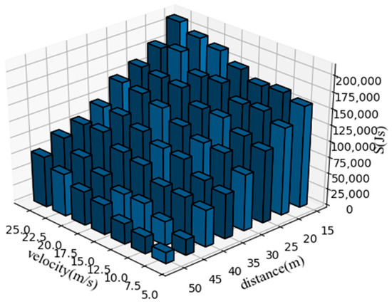
Figure 7.
Average S-values extracted from nine typical scenarios, at different speeds and distances..
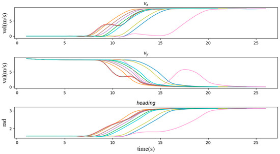
Figure 8.
The speed and heading angle curves of the vehicle when other agents enter the scene (1, 4, 7) from the left side of the intersection.
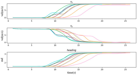
Figure 9.
The speed and heading angle curve of the vehicle when other agents enter the scene (2, 5, 8) from the front of the intersection.
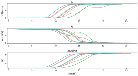
Figure 10.
The speed and heading angle curve of the vehicle when other agents enter the scene (3, 6, 9) from the right side of the intersection.
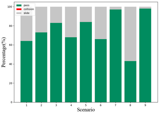
Figure 11.
Results of the decision model of the vehicle in different scenarios.
We examine the cost function graph (Figure 7) first. The cost function diagram for these nine cases demonstrates that, when the vehicle’s speed is constant, the cost function S’s value increases as the initial distance decreases. Similar to this, when the beginning distance is fixed, the cost function S has a bigger value the faster the vehicle j is moving. And if the uniform speed criterion is not met when the cost function crosses a particular level, this car will decide to slow down or change directions; if it continues to pass the intersection at this moment, an accident will happen.
Second, we verify the speed and heading angle graphs in three types of scenarios. From the graphs of the speed variation over time in these three types of examples, the vehicle entering the intersection from the right side of the intersection has the least impact on the vehicle. It can be seen that most of the speed lines change evenly, which represents most situations. The vehicle can easily pass through the intersection without being affected by other vehicles, and the green line shows that the vehicle is waiting for the other vehicle to pass the intersection while coasting at a reduced speed, and then quickly increases the speed to pass through the intersection. Similarly, Figure 9 and Figure 10 also have typical lines that wait for other vehicles to pass the intersection and then speed up to pass through the intersection. Among them, we noticed that the brown line corresponds to the scene where the vehicle is followed by another car after passing the intersection, which is similar to the operation of a skilled human driver. In most other cases, the vehicle maintains the current speed for a while, and then quickly passes through the intersection. Figure 11 can also support this point, the pass rates of scenarios 1 to 9 are 64%, 73%, 83%, 68%, 84%, 66%, 97%, 47% and 98% respectively. The results show that the impact of the left car on the target vehicle is greater than that of the right car, because the pass rates of scenarios 1, 4, and 7 are lower than those of scenarios 3, 6, and 9, respectively. However, the pass rate of scene 8 is much lower than that of other scenes, which means that the situation where the oncoming vehicle in front of the intersection turns left is much more dangerous than other scenes.
To verify the effectiveness of the proposed decision algorithm, we use the TTI threshold method to conduct a total of 8100 simulations under the same simulation conditions. The experimental simulation results are shown in Figure 12. We set experimental scenarios based on TTI from 1 to 9 s. As shown in Figure 12, each TTI condition was simulated 100 times separately. When the TTI threshold of 9 scenarios is less than 2 s, the pass rate reaches the highest value. The highest pass values for these scenarios 1 to 9 are 55%, 59%, 64%, 57%, 65%, 55%, 79%, 45%, and 81%, respectively. However, it can be observed that an increase in the TTI threshold results in a reduced probability of passing and collision, but a higher glide rate, thus reducing the passing efficiency. Therefore, it is necessary to select an appropriate TTI threshold to satisfy both driving safety and efficiency.
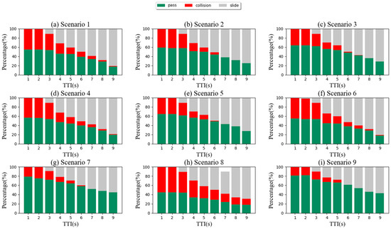
Figure 12.
Performance graph of the TTI threshold method in the nine-unit scene.
The experimental results based on the TTI threshold are the same as the change trend of the decision model’s pass rate. Under the same TTI threshold, the pass rates of scenarios 7 and 9 are much larger than other scenarios in most cases, while the pass rate of scenario 8 is lower than that of other scenarios. This means that scenario 8 has a more dangerous situation than the other scenarios, while scenarios 7 and 9 are relatively safe.
One of the remarkable things we see is that, regardless of the circumstances, this car always crosses the crossing without colliding with another vehicle or coming to a complete stop, with the only difference being the amount of time it takes to lower speed. Additionally, compared to the TTI method, the car is still able to cross the junction smoothly and in less time on average when another vehicle is traveling at a higher speed and a shorter distance, such as in situations 1 and 3 with a time to intersection (TTI) of less than 0.9 s or scenario 2 with a TTI of less than 1.3 s. The automobile can go ahead slowly before another vehicle j has completely past the intersection in scenario 5 with a smaller TTI, while in scenario 4 the car is even capable of moving after vehicle j, being more aggressive than earlier planning algorithms and closer to an experienced human driver.
In the first three scenarios, other vehicles travel in a straight line, while the middle three scenarios involve left turns. In scenario 6, the car behaves more cautiously than in scenarios 4 and 5, at least until vehicle j completely crosses the car’s lane line, at which point the car begins to accelerate and passes the intersection.
Comparing the behavioral decision model to the TTI method reveals that the former significantly increases passage efficiency while maintaining safety, with the latter showing relative improvements of 16.3%, 23.7%, 29.6%, 19.2%, 29.2%, 20.0%, 22.7%, 4.5%, and 20.9% for the nine aforementioned scenarios, respectively. The TTI method ‘s comparatively straightforward risk estimate in the various unit scenarios resulted in comparatively mechanical behavioral choices. In order to ensure traffic safety and increase traffic efficiency, driver operational risk field models offer an edge over TTI method.
4. Discussion
Road intersections are a common feature in urban and suburban areas, and can take many forms, such as a simple two-way stop or a complex interchange. Unprotected intersections are intersections where there are no traffic signals or stop signs to control the flow of traffic. These types of intersections can pose a significant safety risk to all road users, including drivers, pedestrians, and bicyclists. One of the main safety concerns with unprotected intersections is the potential for collisions between vehicles. Without traffic signals or stop signs, drivers may not know who has the right of way, leading to confusion and accidents. Additionally, unprotected intersections can be especially dangerous for pedestrians and bicyclists, who may not be visible to drivers or may not be able to predict the actions of drivers.
AVs are designed to navigate roads and intersections safely, but like any technology, they are not infallible and can make mistakes. In the case of unprotected intersections, AVs may encounter challenges similar to those faced by human drivers, such as determining who has the right of way and predicting the actions of other road users. There have been some reported incidents of AVs encountering issues at unprotected intersections, such as failing to yield to other vehicles or pedestrians [20]. These incidents are relatively rare, but they highlight the importance of continuing to test and improve AV technology to ensure that these vehicles can safely navigate all types of intersections. And according to [20], the probability of an accident is on average 5.5% higher in the left-turn case than in the right-turn case. Therefore, the left-turn scenario at unprotected intersections for autonomous driving is a subject for further study under current technology.
Furthermore, as the left-turn scenario at unprotected intersections is more complex than almost all urban road scenarios, the approach discussed in this paper could theoretically be applied to other urban road scenarios such as ramp meeting, high-speed cruising and T-junctions. Further experimental validation of these scenarios is also required and is the subject of the next work.
5. Conclusions
In this essay, we examine the components and conceptualizations of drivers’ assessments of driving risks. A new vehicle interaction model is suggested based on the analysis of the relationship between the risk field of driving operation and the electric field-like model. This model can increase the decision-making effectiveness by successfully filtering out irrelevant traffic participants while precisely describing the driving risk. Additionally, we show that applying Coulomb forces and electric potential energy to assess driving risks is practical and suitable. Finally, based on the idea of doing the least amount of action possible, we suggest a brand-new modeling technique for driving decisions that can be used in challenging situations involving numerous traffic players. The following is a summary of the study’s main findings.
- The proposed unified driving operation risk field, which consists of two parts: a quantitative assessment of driving risk based on the attributes and motion states of traffic participants in the current scenario using Coulomb force and potential energy, can effectively describe the driving risk during driving.
- Based on the idea of minimum action, we modified a behavioral decision-making model that can quantitatively alter driving objectives. Multi-objective situations can be handled by the model with effectiveness. In addition, from the standpoint of system optimization, a behavioral choice cost function is established. The method enhances the minimal action-based behavioral choice algorithm to make it more flexible to a dynamic environment.
- To test the suggested risk assessment approach and behavior decision model, we created numerous typical urban intersection scenarios. For the purpose of evaluating the effectiveness of the suggested algorithms, several actual urban intersection scenarios are also gathered and simulated.
In contrast to conventional behavioral decision-making techniques, the model establishes a specific area of concern and incorporates efficiency and safety. It can also be used in other situations, such as following the speed limit and changing lanes.
The following three topics will be the focus of future research. The first is to enhance the risk assessment model by taking into account the ambiguity of other traffic participants’ intentions, the second is to enhance the algorithm’s computational effectiveness and its ability to adapt to other complex scenarios, and the third is to conduct hardware-in-the-loop experiments to confirm the proposed algorithm’s effectiveness in real-time.
Author Contributions
Conceptualization, Z.L. and W.Z.; methodology, Z.L.; software, Z.L.; validation, Z.L., W.Z. and B.Z.; formal analysis, Z.L.; investigation, Z.L.; resources, Z.L.; data curation, Z.L.; writing—original draft preparation, Z.L.; writing—review and editing, Z.L.; visualization, Z.L.; supervision, Z.L.; project administration, Z.L.; funding acquisition, W.Z. All authors have read and agreed to the published version of the manuscript.
Funding
This research was funded in part by National Natural Science Foundation of China (No. 51805312, 52172388) And The APC was funded by Zhang.W.
Conflicts of Interest
The authors declare no conflict of interest.
References
- Waymo Finally Launches an Actual Public, Driverless Taxi Service|Ars Technica [EB/OL]. Available online: https://arstechnica.com/cars/2020/10/waymo-finally-launches-an-actual-public-driverless-taxi-service/ (accessed on 8 November 2022).
- Honda Global|March 4, 2021 Honda to Begin Sales of Legend with New Honda SENSING Elite[EB/OL]. Available online: https://global.honda/newsroom/news/2021/4210304eng-slegend.html (accessed on 8 November 2022).
- Toyota Seizes Olympic Glory by Shuttling Athletes Autonomously -Bloomberg[EB/OL]. Available online: https://www.bloomberg.com/news/newsletters/2021-08-02/toyota-seizes-olympic-glory-by-shuttling-athletes-autonomously (accessed on 8 November 2022).
- Baidu, Pony. Ai Approved for Robotaxi Services in Beijing|Reuters[EB/OL]. Available online: https://www.reuters.com/technology/baidu-ponyai-approved-robotaxi-services-beijing-2021-11-25/ (accessed on 8 November 2022).
- We Tried Out a Self-Driving Robotaxi in China—It Was a Very ‘Considerate’ Ride|South China Morning Post[EB/OL]. Available online: https://www.scmp.com/tech/start-ups/article/3040896/we-tried-out-self-driving-robotaxi-china-it-was-very-considerate (accessed on 8 November 2022).
- Kuwata, Y.; Teo, J.; Fiore, G.; Karaman, S.; Frazzoli, E.; How, J.P. Real-Time Motion Planning With Applications to Autonomous Urban Driving. IEEE Trans. Control Syst. Technol. 2009, 17, 1105–1118. [Google Scholar] [CrossRef]
- Andersen, H.; Schwarting, W.; Naser, F.; Eng, Y.H.; Ang, M.H.; Rus, D.; Alonso-Mora, J. Trajectory optimization for autonomous overtaking with visibility maximization. In Proceedings of the 2017 IEEE International Conference on Intelligent Transportation Systems (ITSC), Yokohama, Japan, 16–19 October 2017. [Google Scholar]
- Tumova, J.; Hall, G.C.; Karaman, S.; Frazzoli, E.; Rus, D. Least-violating control strategy synthesis with safety rules. In HSCC ’13: Proceedings of the 16th International Conference on Hybrid Systems: Computation and Control; ACM: New York, NY, USA, 2013; pp. 1–10. [Google Scholar]
- Xu, W.; Pan, J.; Wei, J.; Dolan, J.M. Motion planning under uncertainty for on-road autonomous driving. In Proceedings of the 2014 IEEE International Conference on Robotics and Automation (ICRA), Hong Kong, 31 May–7 June 2014; pp. 2507–2512. [Google Scholar] [CrossRef]
- Mouhagir, H.; Cherfaoui, V.; Talj, R.; Aioun, F.; Guillemard, F. Using evidential occupancy grid for vehicle trajectory planning under uncertainty with tentacles. In Proceedings of the 2017 IEEE 20th International Conference on Intelligent Transportation Systems (ITSC), Yokohama, Japan, 16–19 October 2017; pp. 1–7. [Google Scholar] [CrossRef]
- Ahuja, N.; Chuang, J.-H. Shape representation using a generalized potential field model. IEEE Trans. Pattern Anal. Mach. Intell. 1997, 19, 169–176. [Google Scholar] [CrossRef]
- Fu, G. Safety Management-A Behavior-Based Approach to Accident Prevention; Science Press: Beijing, China, 2013. [Google Scholar]
- Lazarowska, A. Discrete Artificial Potential Field Approach to Mobile Robot Path Planning. IFAC-PapersOnLine 2019, 52, 277–282. [Google Scholar] [CrossRef]
- Jian-Qiang, W.; Jian, W.U.; Yang, L.I. Concept, principle and modeling of driving risk field based on driver-vehicle-road interac-tion. China J. Highw. Transp. 2016, 29, 105. [Google Scholar]
- Zheng, X.; Huang, H.; Wang, J.; Zhao, X.; Xu, Q. Behavioral decision-making model of the intelligent vehicle based on driving risk assessment. Comput. Civ. Infrastruct. Eng. 2021, 36, 820–837. [Google Scholar] [CrossRef]
- Li, G.; Wang, Y.; Zhu, F.; Sui, X.; Wang, N.; Qu, X.; Green, P. Drivers’ visual scanning behavior at signalized and unsignalized intersections: A naturalistic driving study in China. J. Saf. Res. 2019, 71, 219–229. [Google Scholar] [CrossRef] [PubMed]
- Li, G.; Yang, Y.; Zhang, T.; Qu, X.; Cao, D.; Cheng, B.; Li, K. Risk assessment based collision avoidance decision-making for autonomous vehicles in multi-scenarios. Transp. Res. Part C Emerg. Technol. 2021, 122, 102820. [Google Scholar] [CrossRef]
- Levien, R. The Euler Spiral: A Mathematical History; Electrical Engineering and Computer Sciences, University of California at Berkeley: Berkeley, CA, USA, 2008; p. 16. [Google Scholar]
- Zheng, X.; Zhang, D.; Gao, H.; Zhao, Z.; Huang, H.; Wang, J. A Novel Framework for Road Traffic Risk Assessment with HMM-Based Prediction Model. Sensors 2018, 18, 4313. [Google Scholar] [CrossRef] [PubMed]
- Petrović, R.; Mijailović, R.; Pešić, D. Traffic Accidents with Autonomous Vehicles: Type of Collisions, Manoeuvres and Errors of Conventional Vehicles’ Drivers. Transp. Res. Procedia 2020, 45, 161–168. [Google Scholar] [CrossRef]
Disclaimer/Publisher’s Note: The statements, opinions and data contained in all publications are solely those of the individual author(s) and contributor(s) and not of MDPI and/or the editor(s). MDPI and/or the editor(s) disclaim responsibility for any injury to people or property resulting from any ideas, methods, instructions or products referred to in the content. |
© 2023 by the authors. Licensee MDPI, Basel, Switzerland. This article is an open access article distributed under the terms and conditions of the Creative Commons Attribution (CC BY) license (https://creativecommons.org/licenses/by/4.0/).