1. Introduction
The theoretical basis for determining non-conducting bodies in seawater is the problem of diffraction of the field of a grounded cable on a conductive elongated spheroid [
1]. The elongated spheroid is a model of a swimmer in a light diving suit. The excitation of the primary electromagnetic field in seawater is carried out by an electrode antenna (EA) in the form of a grounded cable, the electric field of which is determined by free charges on metal electrodes, compared to which the field from the connecting cable can be neglected [
2]. The field of a grounded cable excites a secondary field on a dielectric spheroid, which can be represented by the fields of two equivalent dipoles, one of which is oriented along the large semi-axis of the spheroid, and the second along the small semi-axis of the spheroid [
1].
In shallow water conditions, seawater forms a conductive layer bound by the seabed and atmosphere. The problem of a horizontal electric dipole placed over a semi-conducting space in the air has been solved [
3,
4]. In our case, the field in the conducting layer is excited by an electrode antenna located inside the conducting layer. The problem of the diffraction of an electromagnetic field on an elongated dielectric spheroid, in this case, should take into account the distortion of the primary field of the EA and the secondary field of the spheroid by a conductive layer. There is no ready-made solution for such a case.
The purpose of this article is to solve the diffraction problem for an elongated non-conducting spheroid in the field of a grounded cable in a conductive layer, with an accuracy level acceptable for practice. This is achieved by strictly solving the problem of diffraction of a homogeneous field at a direct current on an elongated dielectric spheroid in free space, decomposing it into a Taylor series and representing the first dipole term of the expansion at alternating currents, taking into account the influence of the conducting layer.
The authors were able to calculate the flow characteristics of an elongated dielectric spheroid in a conductive layer using real data and comparing it with the results of an experiment on a mock-up of a device protected by a patent [
5].
2. Materials and Methods
When an object enters the field of spreading currents of the transmitting EA, the conductivity of which differs from the conductivity of the environment, the primary field will be distorted. For an infinite homogeneous space, an exact solution to the secondary field of a conducting elongated spheroid at a direct current is known, as is the decomposition of this solution into a Taylor series with the analytical continuation of the first dipole term of this series into the frequency domain [
1]. The solution to the problem of a non-conducting elongated spheroid is reduced to replacing the dipole moment with an equivalent dipole, which can be obtained from the known exact solution of a non-conducting elongated spheroid at a direct current [
6].
Let the spheroid move at a distance
h from the bottom parallel to the boundaries of the layer depth
H. The transmitting and receiving EA are located at the bottom at right angles (
Figure 1). In this case, the secondary field of the spheroid can be represented as a sum of the field equivalent to the horizontal and vertical dipoles relative to the boundaries of the layer [
4].
The determination of the horizontal electric dipole field in the Cartesian coordinate system (
Figure 1) is determined by two components of the vector potential
Ax and
A—satisfying inhomogeneous and homogeneous Helmholtz levels [
3,
4]:
where Δ is the Laplace differential operator in the Cartesian coordinate system;
jx is the density of the equivalent current of the secondary field of the spheroid.
The potential of the electric field
U is determined by the known Lorentz calibration condition for the harmonic field [
3,
4]:
where
is the divergence of the vector potential in the Cartesian coordinate system;
Gn/m is the magnetic constant;
is the relative magnetic permeability of seawater;
F/m is the electric constant;
is the complex permittivity of seawater;
is the relative permittivity of water;
is the wavelength of electromagnetic radiation;
is the specific electrical conductivity of seawater.
Taking into account (1) and (2), Equation (3) will take the form:
Equation (3) satisfies the boundary conditions [
4,
7]:
where
U2 is the potential of the secondary field in seawater;
U1 is the potential of the secondary field in the soil; the interface is a smooth plane whose equation is
Z = 0,
;
are the specific conductivities of the bottom soil and seawater.
The solution to the system of Equation (1) for
Ax and
A with boundary conditions (3) has the form [
7,
8]:
where
is the Fresnel reflection coefficient for homogeneous and inhomogeneous plane waves perpendicular to the plane of incidence;
are coefficients of the propagation of plane waves along the
z axis.
where
.
For a given soil at
z <0 for
Ax and
Az we have:
With the integration of Equations (5)–(8), it is convenient that they are carried out using cylindrical coordinates
r,
φ,
z. The connection with Cartesian coordinates is well known [
9]:
In cylindrical coordinates, expressions (5)–(8) will take the form [
4,
6]:
To transform (11) and (12), we use the Jacobi-Unger decomposition [
9]:
where
Jm(
x) is a Bessel function of the first kind of the
m-th order. Integrate (11) and (12) by φ taking into account (13), then expressions (11) and (12), taking into account (14) will take the form [
9]:
The conductivity of the bottom soil differs little from the conductivity of seawater due to the humidity of the soil compared to the sea water. Therefore,
and
Az = 0, in this case, (9) will take the form [
7]:
that is, the secondary potential of the spheroid is not affected by the lower boundary of the layer. Let us now consider the upper boundary of the seawater–air interface. To do this, in (9), (10), (15), and (16), it is necessary (
Figure 1) to perform substitutions:
replace with
—the coefficient of the propagation of the plane homogeneous waves in the air;
q1—the coefficient of the propagation of the plane waves along the
z axis in the air.
Moreover, since
, then the Fresnel coefficient for the upper interface is
. Thus, (9) and (15) can be rewritten as [
8]:
We determine the secondary potential of the spheroid, taking into account the water-air boundary, by substituting (18) and (19) in (3):
The function (20) is called the flow characteristic of a spheroid when it moves in a conducting layer. When calculating (20), it is taken into account that [
9]
From the integral tables, we have [
10]:
where
R1 is the distance from the center of the spheroid to the first receiving electrode;
is the distance from the “mirror” source of the secondary field of the spheroid to the first receiving electrode (
Figure 1). The equivalent dipole moment of the spheroid
P, taking into account the work of [
7,
11], has the form:
where
U0 is the voltage of the primary harmonic field;
A and
C are the major and minor semi-axes of the elongated spheroid;
is the eccentricity of the spheroid; α
1 and β
1 are auxiliary functions; and:
—the distance from the center of the spheroid to the center of the antenna system;
—the modulus of the field propagation coefficient in seawater.
Thus, to calculate the difference signal of the secondary field on the electrodes of the receiving EA, two factors must be taken into account:
(1) The secondary field of the spheroid is excited by the sum of the fields of the grounded cable and its “mirror” image in the upper boundary of the layer;
(2) The secondary field of the spheroid is equal to the difference between the secondary field of the spheroid excited by the transmitting EA and its “mirror” image at the upper boundary of the layer.
The secondary field of the spheroid (21), taking into account the value of the dipole moment (22) on the receiving electrodes, has the form:
where
is the distance from the center of the spheroid to the first and second receiving electrodes;
is the distance from the “mirror” source of the secondary field to the first and second receiving electrodes;
are coordinates of the first and second receiving electrodes in the Cartesian coordinate system associated with the center of the spheroid. By converting the dipole moment of the spheroid (8) and considering the volume of the spheroid
and
, we get [
12,
13]:
where
is the depolarization coefficient of an elongated dielectric spheroid along the
x-axis.
Similarly, for the dipole moment along the
z-axis we have [
12,
13]:
where
is the depolarization coefficient of an elongated dielectric spheroid along the
z-axis.
3. Practical Implementation
To detect a dielectric object in a conductive layer (
Figure 1), a mobile object-monitoring device was developed and patented, which consists of a linear generator and a receiving EA with orthogonal axes. The generator EA is connected to the symmetrical output of a low-frequency alternating voltage generator, and the receiving EA is connected to the symmetrical input of a differential amplifier. We called such a device a module. To create a protected boundary, several independent modules are placed along it, which are close to the protected water area. Another implementation of an active electromagnetic system for the protection of a water area consists of two independent detection channels: electric and magnetic, complementing each other. This increases the reliability of object detection and their classification based on conductivity [
5,
12].
When developing the receiving part of the device, the following tasks were defined:
1. Signal filtering in order to increase the signal-to-noise ratio;
2. Amplification and conversion of the signal to a form convenient for further processing;
3. Ensuring operational changes in the parameters of the electronic path for the purposes of the experiment.
The basis of the experiment was an electrical circuit with two quadrature channels, which have wide functionality [
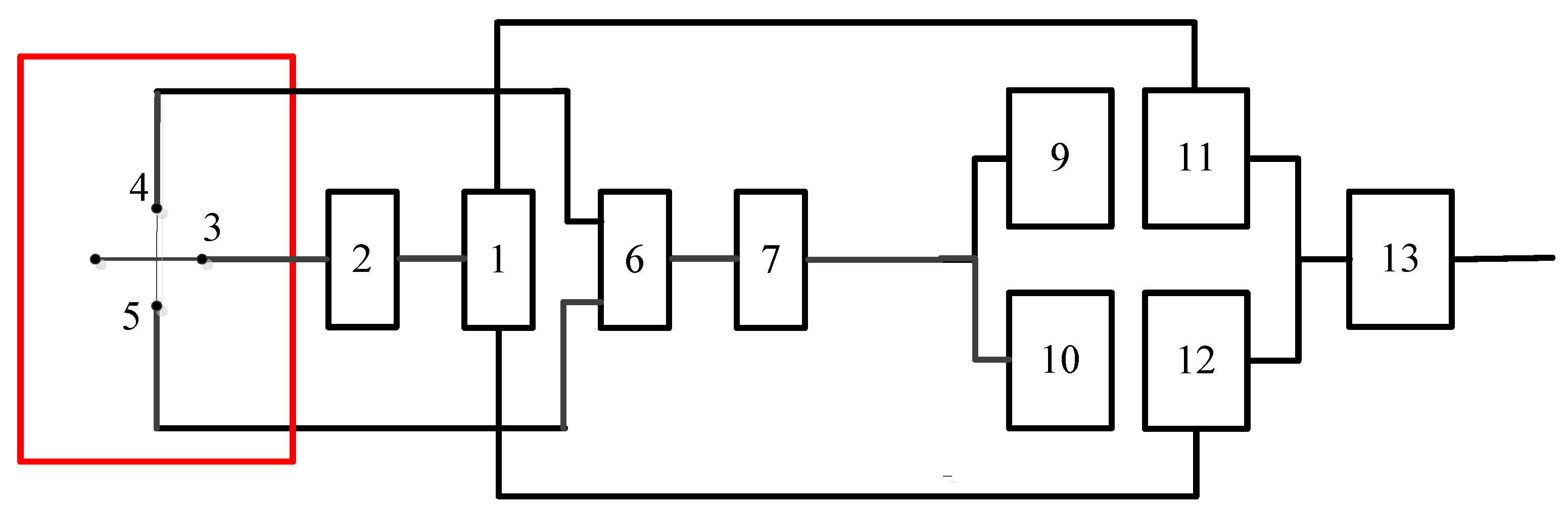
8]. The functional diagram of the receiving part of the device is shown in
Figure 2. The device contains a series-connected generator (1), amplifier (2) and linear EA (3) two identical receiving antennas (4) and (5) connected to the inputs of a differential amplifier (6), whose output through a pole filter is connected to the input of a phase shifter (8), whose output is connected in parallel to an amplifier with a variable coefficient of the amplifier (9) and to the amplifier with a constant gain of (10). The outputs of the amplifiers are connected to the signal inputs of two synchronous detectors (11) and (12).The inputs of the reference signals are connected to the sine and cosine outputs of the generator (1). The outputs of the detectors are connected to the outputs of the adder (13).
The signal from the adder output was recorded in parallel using a digital voltmeter (V7-27/I) and an amplifier (I-37) with an output to the recorder (H37). The device works as follows. A harmonic signal
(where
A is the amplitude,
is the circular frequency) pre-amplified by a power amplifier (2) is fed to the transmitting antenna (3). In the absence of an object, there are harmonic signals
and
at the input terminals of the first and second receiving antennas (4) and (5). At the output of the differential amplifier (6), the difference signal has the form
where
is the amplitude of the difference signal;
K is the amplifier coefficient of the differential amplifier;
—a phase of the difference signal.
The presence of the object leads to the appearance of an additional useful signal at the output of the differential amplifier
where
is the amplitude of the useful signal;
Q is the phase of the useful signal.
After passing the bandpass filter (7), the total signal is received at the input of the processing unit
After passing the phase shifter (8), the total signal is shifted in phase by an angle
.
Further, signal processing is carried out in parallel channels. In the first channel, the signal is amplified by an amplifier (9) and then multiplied by an analog multiplier of the synchronous detector (11) of
and passed through the low-pass filter of the detector (11). As a result, at the output of the first detector, we have
where
is a variable gain of (9).
In the second channel, processing occurs similarly with the difference that the signal
is multiplied in block (12) by the value
. As a result, at output (12) we have
where
is the constant gain of the amplifier (10).
The total output signal (13)
is equal to
In the absence of a signal from the object, we will find the phase
and the amplifier coefficient
from the condition that the difference signal is equal to zero:
from where
Substituting the previous expression
into the found value, we will find the signal from the object at the output of the adder (13):
As the object moves, the amplitude Ac and phase θ of the signal coming from the object will change. Thus, the output of the adder will generate a signal about the presence of an object at any given time.
The electrode antennas were made of symmetrical shielded VRD cable. At the same time, both cable cores were released from the screens at a length of l = 1.5 m. The antenna wires were attached to a wooden bar, 3.5 m long, forming a cross. Next, the wire cores were soldered to a disc copper electrode with a radius of b = 0.125 m. The places for the rations were carefully isolated from the water with bitumen. The electrical circuit was assembled on operational amplifiers.
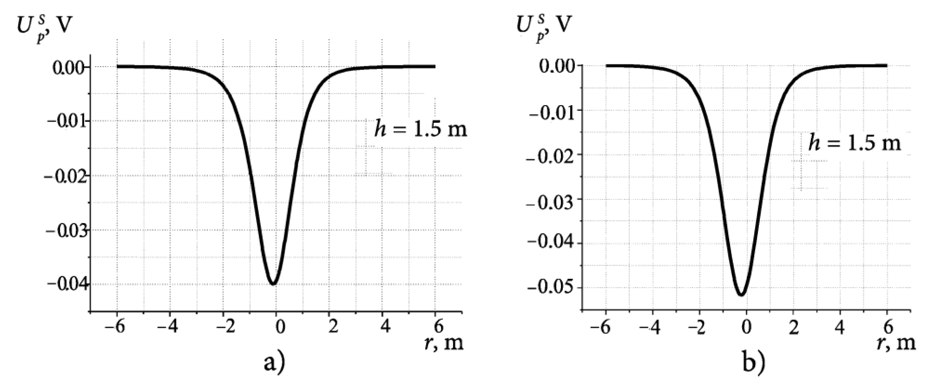
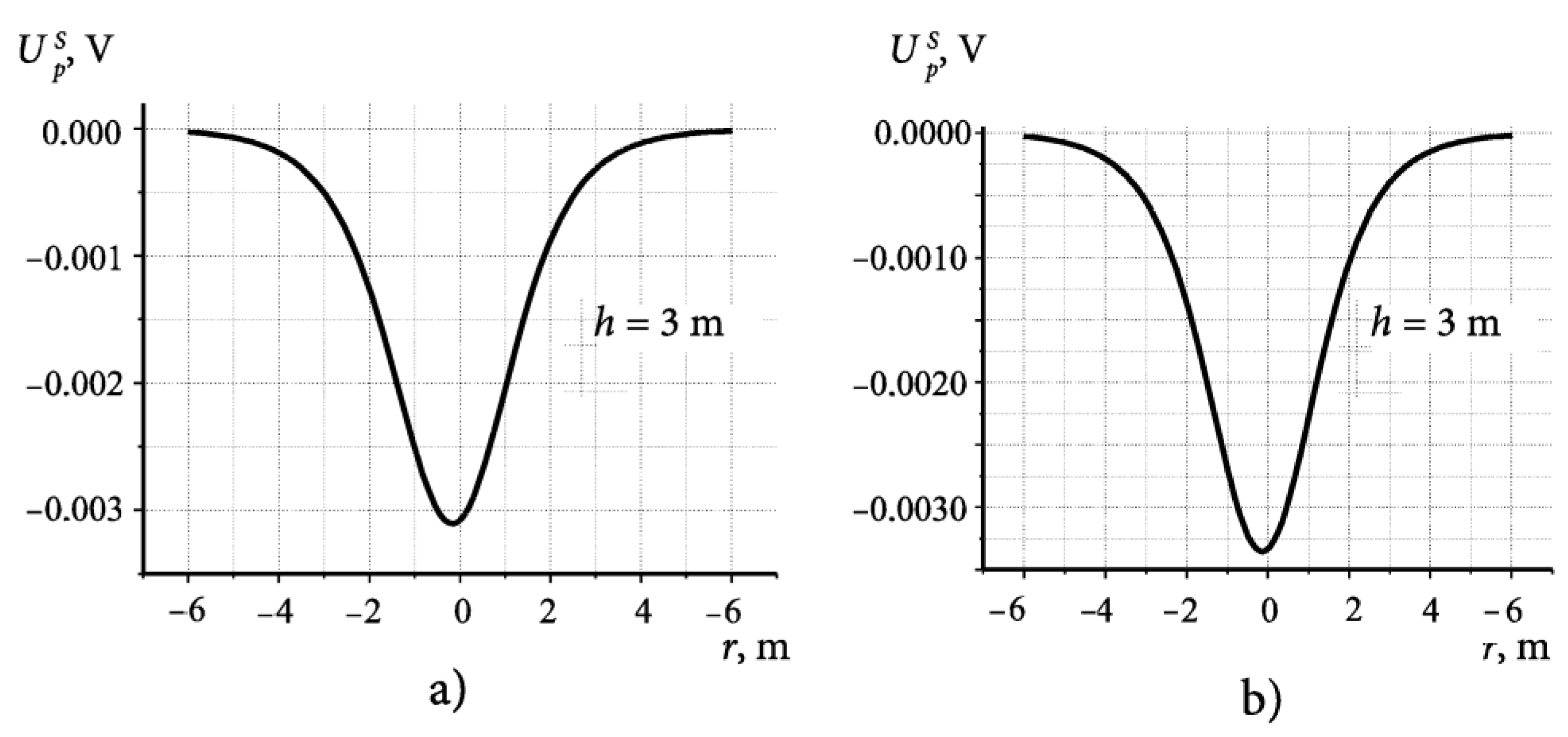
4. Results
To calculate the flow characteristics of the object, it is necessary to set the variables r and φ and constants: H—the depth of the reservoir; h—the height of the object passing over the bottom; b—the radius of the disk electrodes; l—the base of the receiving and transmitting EA; U0—the voltage amplitude of the generator antenna; ω—the circular frequency of the primary harmonic field; Vcf—the volume of a spheroid; n0—the eccentricity of an elongated spheroid; A—the large semi-axis of the spheroid; σ2— the conductivity of seawater. We will accept H = 6 m; h = 1, 5, 3, и 4.5 m; l = 1.5 m; b = 0.125 m; A = 0.9 m; Vcf = 120 l; at the same time c = 0.18 m, c/A≈ 0.2, η0 = 0.98; f = 4·103 Hz ( = 8 · 103 1/c); U0 = 20 B; Nx′ = 0.944; A′ = 0.318 B·м5; k0= 2π·10−2 ≈ 0.2.
Experimental work with the layout of the device was carried out in the waters of the Gulf of Finland. The water conductivity was σ
2 = 0.5 Ohm, and the immersion depth of the antenna module
H varied from 1.5 to 2.5 m. A wooden log with a diameter of 2
C = 0.30 m and a length of 2
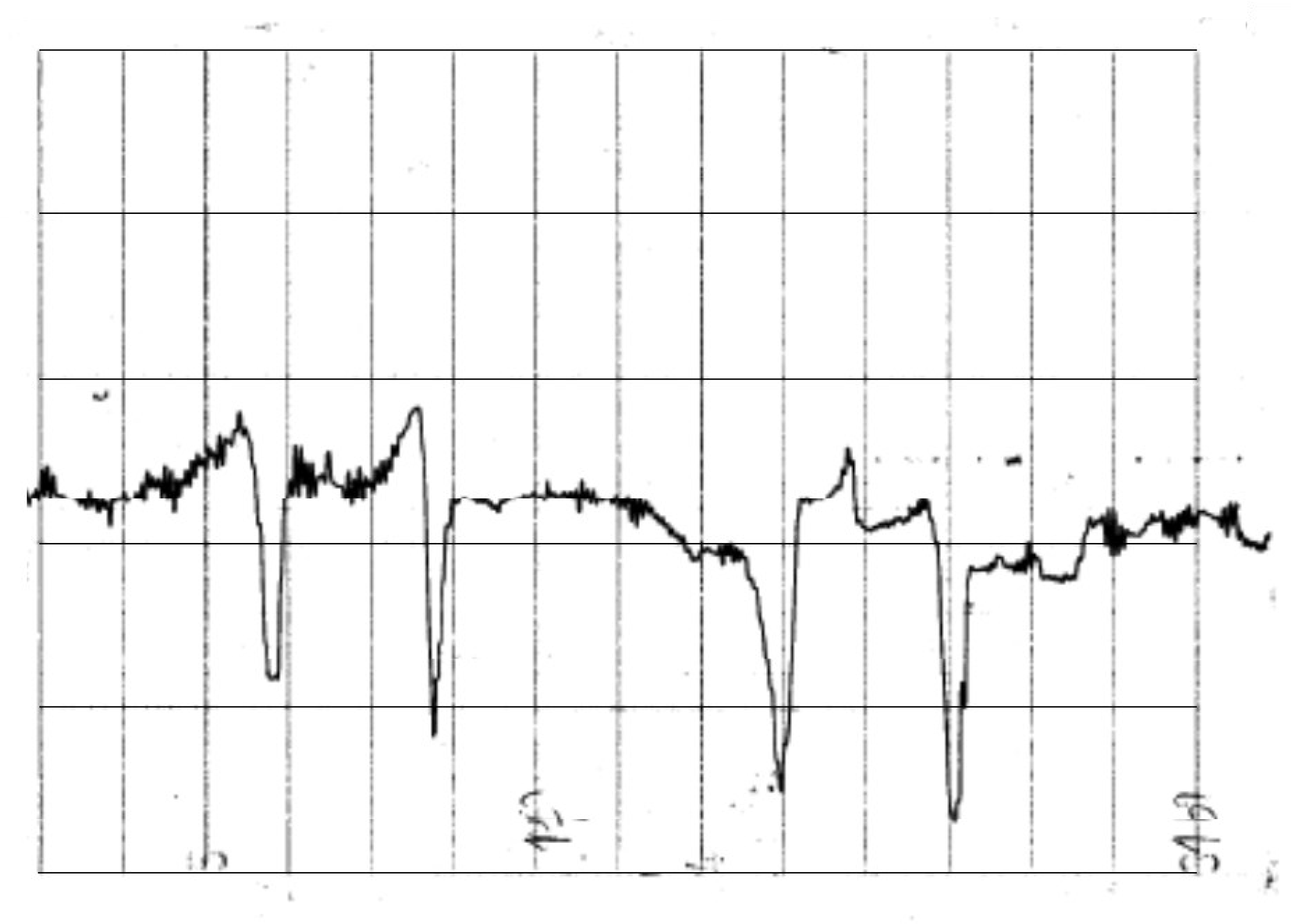
A = 1.2 m was used as a dielectric object. The object was buried with the help of loads while maintaining a positive buoyancy. A fragment of the recorder tape that recorded four passes of the object at a height of
h = 1.5 m is shown in
Figure 3.
The parameters of the experiment: l = 1.5 m; b = 0.125 m; f = 4 103 Hz; U0 = 20 V; k0= 2π 10−2 ≈ 0,2; A = 0.6 m; Vcil = 85 l; at the same time C= 0.15 m, C/A≈ 0.25, recorder sensitivity S = 0.1 v/s.
6. Conclusions
This article develops the fundamental works of Grinberg, G.A. [
3], Koshlyakov, N.S., and others [
4], in which the solution to the problem of the field of a horizontal dipole placed over a semi-conducting medium using the Fourier–Bessel integral transformation is given. Moreover, the problem solved in this article is not identical to the original problem of the horizontal dipole field. Our emitter is a grounded cable of finite length, the field of which is investigated in the work of the first author of the article Kuzmin, Y.I. [
2]. The field of this emitter at distances greater than 3
b can be represented as the sum of the fields of two-point antiphase-powered sources. This fact made it possible to represent the field in the conducting layer with a scalar potential
U, which significantly reduced the amount of calculations. To determine the diffraction field of an elongated dielectric spheroid, an exact solution was taken in a homogeneous field at a constant current of J. Stratton [
3], which was decomposed into a Taylor series. The first dipole term of the series is represented by an alternating current. As a result, the resulting diffraction field was obtained in the form of equivalent fields of horizontal and vertical dipoles. To determine the field in the conducting layer, we used some ideas of Brekhovskikh, L.M. [
8], who studied electromagnetic and acoustic fields in layered media. This article proves that the bottom practically does not affect the field in the conductive layer, and the water-air boundary provides a mirror image of the fields of the vertical and horizontal dipoles of the spheroid and the field of the grounded cable.
Such a solution in elementary functions was obtained for the first time by the original method. As an example, the diffraction field of an elongated dielectric spheroid in a conducting layer excited by the field of a transmitting EA is calculated (
Figure 1). As a result, a good agreement of the theoretical calculations with the results of the experimental data obtained from a life-size model of a security device on the sea shelf of the Gulf of Finland was achieved. We believe that active water area security systems using linear electrode antennas are more promising than acoustic security systems in shallow water at a
H of up to 10 m.
Thus, the developed mathematical model makes it possible to calculate the flow characteristics of conductive and non-conductive bodies in the water with sufficient accuracy for practice, which allows digital filtering of the received signal and significantly increases the signal-to-noise ratio and the detection range of the object. This is the theoretical basis for the creation of various security systems in rivers, canals, and on the sea shelf. This article was prepared as part of the Mining University publication plan for 2022.

