Investigation on the Association of Differential Evolution and Constructal Design for Geometric Optimization of Double Y-Shaped Cooling Cavities Inserted into Walls with Heat Generation

Featured Application

A new complex geometry cavity is optimized by associating the constructal design (CD) method with the differential evolution (DE) algorithm. Statistical analyses are performed to indicate the best parameters of the meta-heuristic to be applied during the optimization process. Kruskal–Wallis and Dunn’s statistical tests were applied to investigate the DE algorithm and its parameters to reproduce the effects of design on the thermal performance of a cooling cavity inserted into a wall with heat generation. Results demonstrated the best parameters of the metaheuristic that improve the algorithm’s performance in the geometric optimization process.

Abstract

In the constructal design method, the comprehension of the effect of design on the system performance is crucial to understanding the contributions of the degrees of freedom or constraints in the system evolution in direction of optimal configurations. However, problems with many degrees of freedom are prohibitive of optimization with exhaustive search, requiring meta-heuristic strategies. Therefore, the investigation of the optimization algorithms is essential. This work investigates the canonical differential evolution algorithm associated with the constructal design for the geometric optimization of an isothermal double Y-shaped cooling cavity inserted into a wall with internal heat generation. The effect of four degrees of freedom over the thermal performance of the system is investigated using sixteen different combinations of differential evolution algorithms: four variations of mutation parameter, two values of amplification factor (F) and two values of crossover rate (CR). The non-parametric statistical methods of Kruskal–Wallis and Dunn test were used to identify the parameters that improve the meta-heuristic efficiency. Results indicated that the proposed methodology selected the proper combination of DE algorithm parameters (CR, F, and mutation) that led to the best effect of degrees of freedom over the thermal performance in all optimization levels investigated.

1. Introduction

The constructal theory is the view that the design of any finite-size flow system is ruled by a physical principle named the constructal law of design and evolution. This law states that the geometrical patterns in the flow system result from its evolution in such a way as to facilitate the access of its internal currents (fluid flow, heat flux, stress flow, people, goods) [1,2]. The method used for the application of constructal theory is named constructal design (CD) and it is based on the definition of constraints, degrees of freedom, and performance indicators [3,4]. Constructal design is not an optimization method, but a method for geometrical investigation of flow systems seeking to comprehend the design evolution and effects of degrees of freedom over the performance of the system and other geometrical parameters. For geometrical optimization, the constructal design is used to define the search space of investigation and the performance indicator, while an optimization method is associated to define the sweep of the search space to obtain the optimal configurations [5,6].

The heat transfer field has been a prolific field for the investigation of the design of flow systems subjected to streams of high/low resistance, generating patterns similar to those seen in many natural flow systems, e.g., trees, rivers, and vascular systems. In this sense, the study of cavities inserted into heat generation walls has been widely investigated to comprehend the generation of design in this kind of system: I, T, Y, X, H, and ψ-shaped cavities [7,8,9,10,11,12,13]. Most of the investigations performed in the literature used the exhaustive search method to perform the geometrical optimization. Although the exhaustive search is a benchmark solution, mainly for the representation of the effect of degrees of freedom over the performance indicators, for the investigation of geometries with a high level of complexity, the number of required simulations can become prohibitive. As a consequence, some meta-heuristic methods have been employed jointly with the constructal design in the recent literature, such as genetic algorithm (GA), simulated annealing (SA), and Luus–Jakola (LJ) [6,14,15,16,17,18,19]. The metaheuristic parameters were also investigated to adequate the computational intelligence strategy to solve other optimization problems in engineering, as can be seen in Echevarria et al. [20]. The authors analyzed the parameters of particle swarm optimization and the ant colony optimization algorithm, and as a result, a new version of PSO emerges.

Concerning the association between computational intelligence and constructal design, Lorenzini et al. [14,15] performed the first studies that associate evolutionary computation with the CD method for geometric optimization of a Y-shaped cavity. The GA was used to reduce the computational effort during the geometric optimization process, as well as allow the study of other conditions as different fraction areas of the cavity and the convection heat transfer coefficient imposed at the cavity’s surfaces, and also its effect over the design of the cavities. Later, Gonzales et al. [16] investigated different functions of the cooling schedule (CS) of the simulated annealing (SA) algorithm over the effect of degrees of freedom on the thermal performance of the Y-shaped cavity previously studied in Lorenzini et al. [14]. The results revealed a more suitable reproduction of the geometry effects over the thermal performance of the system for specific conditions of CS parameters. In Gonzales et al. [17] the SA algorithm was compared with the Luus–Jakola (LJ) heuristic to optimize a double T-shaped cavity. Results demonstrated that the SA algorithm showed better performance to reach the optimal geometries with more regularity than the LJ method. The results of this study were the base for the use of SA associated with the CD method for the complete optimization and geometric evaluation of the double T-shaped cavity in Gonzales et al. [6]. A first attempt at the use of differential evolution (DE) with constructal design (CD) was performed in the work of Gonzales et al. [18], where four different versions of the DE algorithm for the geometrical evaluation of a double T-shaped cavity were investigated. This study observed that the mutation operator DE/rand/1/bin achieved better results than the operator DE/best/2/bin, and the best parameters for crossover rate and amplification factor were CR = 0.7 and F = 1.5. Recent studies that analyze the parameters of the meta-heuristics associated with the CD method show that the algorithm parameter variations affect the geometrical evaluations and reproduction of the geometries effect over the thermal performance of the system [6,16,17,18]. As a consequence, the investigation of the parameters of the algorithms used for geometric optimization is extremely important to guarantee the adequate achievement of optimal configurations and, mainly, for the reproduction of the effect of degrees of freedom over the performance indicators of the system.

In this work, a rigorous investigation of the parameters of the canonical differential evolution algorithm when it is associated with constructal design for geometrical optimization of a double Y-shaped cavity (not previously studied in the literature) is performed. It investigated the parameters of crossover rate, amplification factor, and four different mutation operators. The combination of the algorithm parameters generated 16 versions of the DE that were analyzed. The DE algorithm versions were executed to obtain the optimization of four degrees of freedom. The results of the experiments were analyzed by non-parametric statistical tests of the Kruskal–Wallis and post hoc test of Dunn. Firstly, the Shapiro–Wilk procedure is applied to verify the population distribution. The statistical tools applied make possible the identification and discernment of the parameters that improve the performance of the DE algorithm. In the recent literature, a non-parametric statistical test was used to validate and compare the algorithm results [21,22]. The parameters recommended in the preliminary work of Gonzales et al. [18] were compared with new values of F and CR and new mutation operators. The findings contribute to new recommendations about the DE parameters that enhance the algorithm performance associated with the CD method for geometrical optimization of the cavity problem. The best parameters found in this work will be applied to optimize all seven degrees of freedom of the complex double Y-Shaped cavity in a future study.

2. Mathematical and Numerical Modeling

2.1. Description of the Cavity Inserted in the Solid Domain Problem

Figure 1 shows the double Y-shaped cavity in a two-dimensional domain. The third dimension (W) is perpendicular to the plane of Figure 1. The gray region in Figure 1 represents the solid domain which has a constant and uniform heat generation at the volumetric rate given by q^‴ (W∙m⁻³). Due to the symmetry of the domain about the y-axis, only half of the computational domain of the solid is solved. The thermal conductivity k is constant in the solid domain, and its outer boundary surfaces are perfectly insulated (adiabatic conditions). The double Y-shaped cavity surfaces are kept at a minimum temperature (T_min). In this case, the cavity acts by removing the heat generated by the solid domain. The lowest imposed temperature simulates a condition where a phase change convection heat transfer flows through the cavity. As a simplifying hypothesis, the heat transfer coefficient on the cavity wall is assumed high enough in such way the convective resistance can be neglected compared to the solid conduction resistance. The problem studied here is subjected to the simplification hypothesis listed below:

1

The problem is considered at the steady-state;

2

The heat generation per unit volume (q^‴) is constant in the solid domain;

3

The thermal conductivity is also constant;

4

The domain is two-dimensional.

Therefore, the problem is modeled by the heat diffusion equation, which after the imposition of the simplification hypothesis is given by [23]:

$$\frac{{\partial }^{2}T}{\partial x^2}+\frac{{\partial }^{2}T}{\partial y^2}+\frac{q^{‴}}{k}=0$$

(1)

where T is the temperature (K), x and y are the spatial coordinates (m), q^‴ is the heat generation per unit volume (W∙m⁻³) and k is the thermal conductivity (W∙m⁻¹∙K⁻¹).

The objective of the present study is to determine the optimal geometry (H/L, H₀/L₀, H₁/L₁, H₂/L₂, S₁/H₀, α, and β) that minimizes the maximum excess of temperature (T_max − T_min)/(q^‴A). In the present work, four parameters are investigated (α, β, S₁/H₀, and H₀/L₀) while the others are kept constant. According to the CD method, the geometrical investigation is subjected to two constraints, the total area of the domain and cavity area, which are given, respectively, by:

$$A=HL$$

(2)

$$A_c=H_0{L}_0+2H_1{L}_1+2H_2{L}_2$$

(3)

The dimensionless form of the Equations (2) and (3) are represented by the following equations:

$$\tilde{H}\tilde{L}=1$$

(4)

$${\phi }_c=\frac{A_c}{A}={\tilde{H}}_0{\tilde{L}}_0+2{\phi }_1+2{\phi }_2$$

(5)

where:

$${\phi }_1={\tilde{H}}_1{\tilde{L}}_1$$

(6)

$${\phi }_2={\tilde{H}}_2{\tilde{L}}_2$$

(7)

The temperature fields in the solid domain were determined by solving the heat diffusion equation given in dimensionless form by:

$$\frac{{\partial }^2\theta }{\partial {\tilde{x}}^2}+\frac{{\partial }^2\theta }{\partial {\tilde{y}}^2}+1=0$$

(8)

In the dimensionless process of the heat diffusion equation, the term q^‴/k is evidenced in all terms, given rise to the unity in the third term of Equation (8). The dimensionless variables can be written as:

$$\theta =\frac{T-T_{min}}{q^{‴}·\frac{A}{k}}$$

(9)

$$\tilde{x},\tilde{y}, \tilde{H}, {\tilde{H}}_0, {\tilde{H}}_1, {\tilde{H}}_2, \tilde{L}, {\tilde{L}}_0, {\tilde{L}}_1, {\tilde{L}}_2, {\tilde{S}}_1=\frac{x, y, H, H_0, H_1, H_2, L, L_0, L_1, L_2, S_1}{A^{1/2}}$$

(10)

For the sake of brevity, the boundary conditions equations of null flux in the outer surfaces are not addressed here. More details can be seen in the work of Ref. [16] which studied a similar problem but with a T-shaped cavity configuration. The boundary condition of minimal temperature (θ = θ_min) is imposed at all cavity surfaces and described in the following equations:

$$\theta ={\theta }_{min} in 0 \le \tilde{y} \le {\tilde{S}}_1-\frac{{\tilde{H}}_1}{2sin\left(90°-\alpha \right)} and \tilde{x}=-\frac{{\tilde{L}}_0}{2} or \tilde{x}=\frac{{\tilde{L}}_0}{2}$$

(11)

$$\begin{gathered} \theta ={\theta }_{min} in {\tilde{S}}_1-\frac{{\tilde{H}}_1}{2sin\left(90°-\alpha \right)} \le \tilde{y} \le {\tilde{L}}_{1}sin\alpha +{\tilde{S}}_1-\frac{{\tilde{H}}_1}{2sin\left(90°-\alpha \right)} \\ and-\frac{{\tilde{L}}_0}{2}-{\tilde{L}}_{1}cos\alpha \le \tilde{x} \le -\frac{{\tilde{L}}_0}{2} or \frac{{\tilde{L}}_0}{2} \le \tilde{x} \le \frac{{\tilde{L}}_0}{2}+{\tilde{L}}_{1}cos\alpha \end{gathered}$$

(12)

$$\begin{gathered} \theta ={\theta }_{min} in \tilde{x}=-\frac{{\tilde{L}}_0}{2}-{\tilde{L}}_{1}cos\alpha or \tilde{x}=\frac{{\tilde{L}}_0}{2}+{\tilde{L}}_{1}cos\alpha \\ and {\tilde{L}}_{1}sin\alpha +{\tilde{S}}_1-\frac{{\tilde{H}}_1}{2sin\left(90°-\alpha \right)} \le \tilde{y} \le {\tilde{L}}_{1}sin\alpha +{\tilde{S}}_1+\frac{{\tilde{H}}_1}{2sin\left(90°-\alpha \right)} \end{gathered}$$

(13)

$$\begin{gathered} \theta ={\theta }_{min} in {\tilde{S}}_1+\frac{{\tilde{H}}_1}{2sin\left(90°-\alpha \right)} \le \tilde{y} \le {\tilde{H}}_0-\frac{{\tilde{H}}_2}{sin\left(90°-\beta \right)} \\ and \tilde{x}=-\frac{{\tilde{L}}_0}{2} or \tilde{x}=\frac{{\tilde{L}}_0}{2} \end{gathered}$$

(14)

$$\begin{gathered} \theta ={\theta }_{min} in-\frac{{\tilde{L}}_0}{2}-{\tilde{L}}_{2}cos\beta \le \tilde{x} \le -\frac{{\tilde{L}}_0}{2} or \frac{{\tilde{L}}_0}{2} \le \tilde{x} \le \frac{{\tilde{L}}_0}{2}+{\tilde{L}}_{2}cos\beta \\ and {\tilde{H}}_0-\frac{{\tilde{H}}_2}{sin\left(90°-\beta \right)} \le \tilde{y} \le {\tilde{H}}_0-\frac{{\tilde{H}}_2}{sin\left(90°-\beta \right)}+{\tilde{L}}_{2}sin\beta \end{gathered}$$

(15)

$$\begin{gathered} \theta ={\theta }_{min} in \tilde{x}=-\frac{{\tilde{L}}_0}{2}-{\tilde{L}}_{2}cos\beta or \tilde{x}=\frac{{\tilde{L}}_0}{2}+{\tilde{L}}_{2}cos\beta \\ and {\tilde{H}}_0-\frac{{\tilde{H}}_2}{sin\left(90°-\beta \right)}+{\tilde{L}}_{2}sin\beta \le \tilde{y} \le {\tilde{H}}_0+{\tilde{L}}_{2}sin\beta \end{gathered}$$

(16)

$$\begin{gathered} \theta ={\theta }_{min} in {\tilde{H}}_0 \le \tilde{y} \le {\tilde{H}}_0+{\tilde{L}}_{2}sin\beta \\ and-\frac{{\tilde{L}}_0}{2}-{\tilde{L}}_{2}cos\beta \le \tilde{x} \le -\frac{{\tilde{L}}_0}{2} or \frac{{\tilde{L}}_0}{2} \le \tilde{x} \le \frac{{\tilde{L}}_0}{2}+{\tilde{L}}_{2}cos\beta \end{gathered}$$

(17)

$$\theta ={\theta }_{min} in \tilde{y}={\tilde{H}}_0 and-\frac{{\tilde{L}}_0}{2}\le \tilde{x}\le \frac{{\tilde{L}}_0}{2}$$

(18)

The objective is to minimize the dimensionless maximum excess of temperature, given by:

$${\theta }_{max}=\frac{T_{max}-T_{mix}}{q^{‴}\cdot \frac{A}{k}}$$

(19)

In this paper, the notation Nm is used for the dimensionless maximum excess of temperature N times minimizes and No for geometry N times optimized, e.g., (θ_max)_2m and (β)_2o represents the dimensionless maximum excess of temperature two times minimized and the angle β two times optimized. For the determination of the (θ_max)_7m, the seven degrees of freedom must be optimized (H/L, H₀/L₀, H₁/L₁, H₂/L₂, S₁/H₀, α, and β) considering the cavity area constraints (φ_c, φ₁, and φ₂) and the total area of the solid. It is worth mentioning that one of the main aspects of constructal design is the comprehension about the influence of the degrees of freedom over the performance indicator and other degrees of freedom from the second level of investigation onward. Therefore, the reliability of the optimization algorithm studied here is not only important to find the optimal configuration, but also for the above-mentioned investigation about the design of the flow system.

2.2. Numerical Solution of Heat Transfer in Solid Domain

The temperature field is determined numerically by solving Equation (8) for every assumed geometry (H/L, H₀/L₀, H₁/L₁, H₂/L₂, S₁/H₀, α, and β) during the optimization process. With the temperature field calculated, the θ_max is defined by a function given by Equation (19), which represents the objective function (OF) of the optimization problem. The numerical solution is obtained in this work with the finite element method (FEM) [24]. The code for numerical solutions is developed in the MATLAB^® environment, using the PDE (partial differential equations) toolbox [25], based on triangular quadratic elements. The grid is non-uniform in both $\tilde{x}$ and $\tilde{y}$ directions and varied from one geometry to the next. The appropriate mesh size is defined by successive refinements, multiplying the number of elements four times from a current mesh size to the next. The used mesh grid was determined after successive refinements and tests to reach the independent mesh solution in the computational domain. The criterion employed to find the correct mesh with the total number of elements is represented by the following equation:

$$\left|\frac{\left({\theta }_{max}^i-{\theta }_{max}^{i+1}\right)}{{\theta }_{max}^i}\right|<2\times {10}^{-4}$$

(20)

The appropriated mesh size is found when the Equation (20) is satisfied, θⁱ_max representing the max temperature value evaluated with current mesh size, and θⁱ⁺¹_max corresponds to the refined mesh value, i.e., approximately four times more elements than previous mesh.

Table 1. Results of grid independence test.

Number of Elements	θmax	|(θimax − θi+1max)|/θimax
1.265	0.16767	1.2 × 10−3
5.132	0.16787	4.579 × 10−4
20.486	0.16795	1.866 × 10−4
82.592	0.16798	7.307 × 10−5
325.431	0.16799	-

shows the test of the solution independent of the mesh, it can be noted that the independent solution is achieved before three refinements with a total of 20.486 triangular elements. Figure 2a,b shows the coarse and fine mesh with triangular elements, respectively. Figure 2b also show the one half of the domain numerically solved. The mesh test was implemented with a follow geometric configuration: φ_c = 0.1; φ₁ = 0.015; φ₂ = 0.015; H/L = 1; H₀/L₀ = 6; S₁/H₀ = 0.5; H₁/L₁ = 0.4; H₂/L₂ = 0.4; α = β = 0.

The implemented code accuracy was validated from the comparison of results of other cooling cavities, investigated in the work of [7,10] for a T-shaped cavity, and the result of [6], for a double T-shaped cavity. However, an extra area constraint is required, named here as ψ for the adequate comparison of the numerical model present in this work with the literature references. This new constraint means the occupied area of solid by the cavity. Therefore, considering α = β = 0°, for the double Y-shaped cavity, the ψ is given by the following equation:

$$\psi =\frac{H_0\left(2L_2+L_0\right)}{HL}$$

(21)

The geometry used to the accuracy test is similar to the second construction in T-shape [7] and has the following geometric configuration: ψ = 0.5, φ_c = 0.1; φ₁ = 0.02; φ₂ = 0.02; H/L = 1; H₀/L₀ = 20; S₁/H₀ =0.45; H₁/L₁ = 14; H₂/L₂ = 0.14; α = β = 0°.

Table 2. Validation of the computational method used in present work with references in the literature [6,7,10].

Number of Elements	θmax
Present Work	0.0756
Gonzales et al. [6]	0.0756
Lorenzini et al. [10]	0.0762
Biserni et al. [7]	0.0755

shows the comparison between results obtained with numerical method and codes employed in this work with results in the literature.

2.3. Application of Constructal Design to Design of Double Y-Shaped Cavity

The optimization methodology is oriented by the CD method that defines a hierarchy path between the degrees of freedom to perform the geometrical evaluation, i.e., the CD defines the search space and the order of DOFs investigated. The optimization process starts with the investigation of one degree of freedom while the other is kept at constant magnitudes. In the present work, it is optimized the degrees of freedom α, β, S₁/H₀, and H₀/L₀, i.e., a four-level optimization. For all optimization levels, the constraints were defined as φ_c = 0.01, φ₁ = φ₂ = 0.015. The degrees of freedom H₁/L₁ and H₂/L₂, which describe the double Y-shaped cavity branches, were kept with minimal values on the search space, following the recommendations of the best configuration of double T-shaped cavity studied in [6,17,18]. For the first level of the optimization process, the cavity branch angles (α and β) were optimized synchronously with the same values, as if they were just one degree of freedom (α = β). Then, the meta-heuristic is applied to find the optimal geometry of (α)_o and (β)_o that returns the (θ_max)_m. The search space of angles investigated was α = β ∈ [−80°, 80°] with the discrete variation of Δα = Δβ = 1°. The values of other ratios are fixed, H/L = 1.0, H₀/L₀ = 10, and S₁/H₀ = 0.5.

The second level of the optimization process searched for the optimal values of α and β independently (α ≠ β) in the same search space as the previous optimization level. The other geometric parameters and constraints were kept constant during the optimization process and with the same values used in the previous optimization level. Therefore, the optimization method seeks the optimal geometries of (α)_o and (β)_2o that lead to (θ_max)_2m. For the third optimization level, the degree of freedom S₁/H₀ was added to the investigation, so the optimization algorithms seek for (S₁/H₀)_o, (α)_2o, and (β)_3o that reaches the three times minimized dimensionless maximum excess of temperature, (θ_max)_3m. The other geometric parameters continued to be kept fixed with the same magnitudes of the previous optimization process, except for H₀/L₀ = 16. Finally, the last experiment performs a fourth optimization level, i.e., taking also into account the ratio H₀/L₀. Therefore, the three degrees of freedom α, β, and S₁/H₀ were optimized for different magnitudes of H₀/L₀ in the last investigation.

Considering that the CD method has the main aim to understand the effect of the degrees of freedom over the optimal geometries and performance indicators, the experiments performed here focus on adapting the meta-heuristic to the problem of interest. Supposing the algorithm presents an adequate performance to reach the optimal geometries, it will probably be capable of reproducing the correct effects of geometries over the system performance for complete optimization and evaluates all seven degrees of freedom in future studies with a much lower computational effort than that required with the exhaustive search.

3. Optimization Methodology

3.1. Differential Evolution Algorithm

The differential evolution (DE) algorithm was proposed by Storn and Price [26] as an efficient meta-heuristic for continuous search spaces of non-linear and/or non-differentiable functions. Storn and Price [26] tested extensively several types of functions and optimization problems, showing the efficiency of the method compared with other well-known optimization heuristics. The canonical form of the DE method has the following parameters: population size (NP), the total number of generations (NG), crossover rate (CR), mutation operator (M), and amplification factor (F). As a population-based meta-heuristic, the DE method uses NP vectors of optimization problem dimension size to compose its population. In the canonical form of the method, the population size does not change during the algorithm iteration, as well as the total number of generations (NG). The NG also determines the stopping criterion of the DE method. The initial population must be generated randomly and uniformly distributed over the search space [25]. The steps of the DE algorithm are described below:

• Generate a first population with NP vectors x_i,G, and i = 1, 2, 3, ..., NP, being G the current generation.
• Apply the mutation operator for each vector in the population as given by:

  $$v_{i,G+1}=x_{r_1,G}+F\times \left(x_{r_2,G}-x_{r_3,G}\right) \forall F>0$$

  (22)

  where the indexes r₁, r₂, r₃ ∈ 1, 2, 3, ..., NP are integers randomly generated and mutually different. The F controls the amplification of the differential term $\left(x_{r_2,G}-x_{r_3,G}\right)$.
• Create u_i,G+1 = (u_1i,G+1, u_2i,G+1, ..., u_Di,G+1) which is a trial vector, being D the length of the vector (dimension of the problem). The trial vector is a combination between x_i,G and v_i,G+1 determined by:

  $$u_{ji,G+1}=\left\{\begin{array}{c}{v}_{ji,G} if rnd\left(0,1\right) \le CR or j=j_r\\ x_{ji,G} otherwise\end{array}\right.$$

  (23)

  where rnd() is a function that generates a random number between 0 and 1, and CR is the crossover probability. The j_r ∈ [1...D] is randomly generated and assurances that v_ji,G differs from x_ji,G by inserting at least one of the v_i,G elements.
• Select the best solution for the next generation G+1 comparing x_i,G with u_i,G+1 by a Greedy criterion:

  $$x_{i,G+1}=\left\{\begin{array}{c}{u}_{i,G+1} if OF\left(u_{i,G+1}\right) \le OF(\left(x_{i,G+1}\right)\\ x_{ji,G} otherwise\end{array}\right.$$

  (24)

The steps are repeated while G $\le$ NG is true. The mutation operator shown in Equation (12) is considered the DE/rand/1/bin by notation DE/x/y/z [25]. The x represents the vector target of the mutation, y is the number of subtractions performed, and z is the crossover type, which for Equation (12) is binomial. More three mutation operators are analyzed in this work, called DE/best/1/bin, DE/best/2/bin, and DE/current-to-best/1/bin, respectively, described by the following equations:

$$v_{i,G+1}=x_{best,G}+F\times \left(x_{r_1,G}-x_{r_2,G}\right)$$

(25)

$$v_{i,G+1}=x_{best,G}+F\times \left(x_{r_1,G}+x_{r_2,G}-x_{r_3,G}-x_{r_4,G}\right)$$

(26)

$$v_{i,G+1}=x_{i,G}+F\times \left(x_{best,G}+x_{i,G}\right)+F\times \left(x_{r_1,G}-x_{r_2,G} \right)$$

(27)

Figure 3 shows the flowchart of the differential evolution algorithm applied to the geometric optimization of the double Y-shaped cavity. The flowcharts represent the algorithm that integrates the meta-heuristic to the solver of the heat transfer problem. The solution of the heat diffusion equation, Equation (8), and corresponding boundary conditions are performed by the finite element method (FEM) implemented in the PDE toolbox of MATLAB^® platform [25]. This part of the algorithm solves the heat transfer problem and determines the thermal fields on the computational domain, returning the value of θ_max for each geometric configuration and acting as an Objective Function (OF) in the geometric optimization problem. All the DE code was made in the MATLAB^® platform and the results were saved in CSV format for posterior statistical analyzes in the Software-R environment [27].

3.2. Experiments and Statistical Analysis

This study analyzed various combinations of DE algorithm parameters, which resulted in sixteen versions of DE. The different versions of DE were named according to the following code DExy, where x represents the variation of mutation parameter and y the combination of the F and CR parameters.

Table 3. Parameters combinations and versions of DE algorithm.

DExy Encoded Name	Crossover	Amplification Factor
DEx1	0.7	1.5
DEx2	0.7	1
DEx3	0.9	1.5
DEx4	0.9	1
	Mutation Operator
DE1y	rand/1/bin
DE2y	best/1/bin
DE3y	best/2/bin
DE4y	current-to-best/1/bin

shows the parameters investigated in this work, and the versions of the DE algorithm with the DExy encode. According to Table 3, the algorithm version with the name DE14 means that the parameters of this version were: rand/1/bin, CR = 0.9, and F = 1.0.

The experiments consist of thirty runs of each algorithm to achieve the dimensionless maximum excess of temperature n times minimized (θ_max)_nm for each optimization level, as well as the statistical analysis of results to identify the better versions of the DE. The statistical analysis starts with the use of the Shapiro–Wilk test to determine the population distribution, Shapiro and Wilk [28]. If the test validates the free distribution, then the non-parametric test of Kruskal–Wallis (KW) [29] is performed to identify if exists a significant difference between the algorithms’ results. The KW test verifies the null hypotheses h₀ represented by:

$$\begin{array}{c}{h}_0={\mu }_1={\mu }_2=\dots ={\mu }_a\\ h_1={\mu }_i \ne {\mu }_a\end{array}$$

(28)

If the h₀ is accepted, there is evidence that the algorithms results come from the same population. Otherwise, the alternative hypotheses h₁ is accepted and there is at least one algorithm whose results are different from the other.

The KW test helps to find a difference in one of the algorithms evaluated. However, it is not enough to know which one of the versions are different. For this purpose, the post hoc test of Dunn is applied to identify differences between the DE algorithm versions. Dunn test implements multiple comparisons based on rank sums [30]. The significance level used for all statistical test was α_s = 0.05. All tests were performed in the Software-R environment [27].

The Dunn test uses the following equation to determine the difference between the analyzed factors (algorithm):

$$\left| R-R^{\prime }\right| \ge Z_{{\alpha }^{\prime }} {\left[\frac{N\left(N+1\right)}{12}\right]}^{1/2}\times {\left(\frac{1}{n}+\frac{1}{n}\right)}^{1/2}$$

(29)

where R and R′ are the mean of ranks of each factor (algorithm), N is the total number of observations, n and n′ are the numbers of observations for each of the algorithm version. The α´ represents α_s (a − 1), where α_s is the significance level and a is the number of factors (algorithm versions). Z is the normal distribution. The right term of the equation is the minimal significance difference between the mean of ranks of the factors for a given α_s. If the absolute difference between R and R′ is greater or equal than the minimal significance difference, right-hand term of the Equation (29), then the h₀ is rejected, and the compared factors (algorithms) have statistically significant difference.

4. Results and Discussion

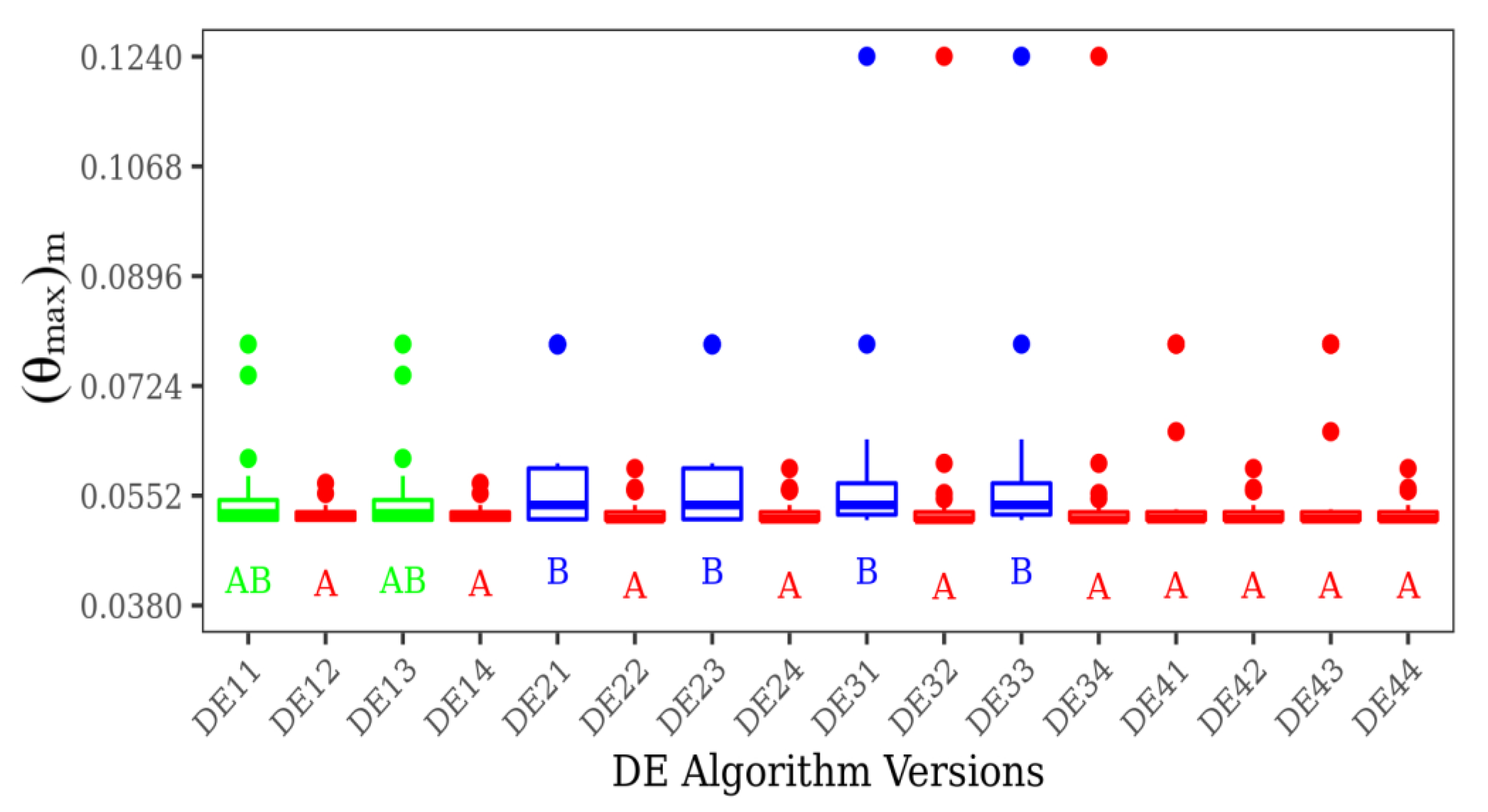
4.1. Optimization Results for One Degree of Freedom

The first experiment consists of the optimization of one degree of freedom of the double Y-shaped cavity, represented by the angles α and β. For this first level optimization, all DE versions were configured with NP = 5 and NG = 10. The results of 30 runs obtained with each of the DE versions for the average (θ_max)_m and the statistical metrics as variance, standard deviation, and root mean square error (RMSE) are presented in

Table 4. Statistical metrics of the results achieved for (θ_max)_m.

DE Versions	Average (θmax)m	Variance (×10−4)	Standard Deviation (×10−3)	RMSE (×10−3)
DE12; DE14	0.05232	0.017	1.33	1.61
DE22; DE24	0.05253	0.038	1.96	2.24
DE41; DE43	0.05491	0.728	8.53	9.10
DE31; DE33	0.05770	1.870	13.70	14.9

. For the sake of brevity, only the best two groups and the worst two ones are shown in Table 4, sorted in ascending order. The versions of the DE algorithm which reach the best results are DE12 and DE14. They conducted the lowest values for the average of (θ_max)_m, as well as the lowest magnitudes of standard deviation and RMSE. These algorithms only have in common the mutation operator (rand/1/bin) and the parameter F = 1.0. The CR parameter does not have an influence on the results of versions ED12 and ED14. The second group with satisfactory results is the one having versions DE22 and DE24. These versions have as mutation operators the parameter best/1/bin and F = 1.0. Again, the difference in CR parameters does not affect the results of these versions of the DE algorithm. The results of the Table 4 indicated that the DE versions with F = 1.0 are more efficient to obtain the lowest mean magnitude of (θ_max)_m. On the other hand, the last two groups in Table 4 conducted the worst performance. The versions DE31, DE33, DE41, and DE43 achieved more divergent values from the (θ_max)_m average, which indicate that the versions obtained several local minimum magnitudes of (θ_max)_m. These versions consider the mutation parameters best/2/bin and current-to-best/1/bin, Equations (16) and (17). For this level of investigation, the mutation operator best/2/bin led to the worst performance in comparison with the others.

Shapiro–Wilk (SW) and Kruskal–Wallis (KW) statistical tests were applied to determine the statistically significant difference between the 16 versions of DE algorithm results, as can be seen in

Table 5. Statistical hypotheses test of DE versions for (θ_max)_m.

Shapiro–Wilk: Normality Test
DE Versions	p-Value		Distribution
DE12; DE14	2.785 × 10−6		Non-normal
DE22; DE24	3.275 × 10−7		Non-normal
DE31; DE33	1.489 × 10−9		Non-normal
DE41; DE43	1.870 × 10−4		N on-normal
Kruskal–Wallis: Rank Sum Test
DE Versions	p-Value	αs	Differences
DE [12; 14; 22; 24; 31; 33; 41; 43]	1.932 × 10−6	0.05	Significant
All versions	1.109 × 10−7	0.05	Significant

. According to the SW test, all algorithm results have a free distribution that allows non-parametric statistical analysis. The results of the KW test presented in Table 5 confirm a significant difference between the results of the algorithm for the first-level optimization of the double Y-shaped cavity, corroborating the findings of Table 4. The next step in the analysis of the algorithm’s results is to identify which versions of DE differ from the other. For this purpose, the Dunn test is performed, and the results are illustrated in Figure 4 and Figure 5. The distribution of each algorithm version is shown through the BoxPlot graph with the color representing the classification groups generated by the Dunn test. Figure 4 shows two groups of performance, A and B, which indicates that the algorithms in the same group have similar statistical performance, while algorithms in different groups have statistical performance differences. Figure 4 indicates differences between DE12 and DE31 versions, but it is impossible to distinguish in statistical viewpoint differences between the algorithms DE12, DE14, DE22, DE24, DE41, and DE43, even with some differences in the achievement of global point of minimum magnitude of (θ_max)_m.

Figure 5 presents the Dunn test for all versions of DE, given a broader view about the comparison of all algorithms studied. Results of Dunn test indicate the sensitivity of the analyzed versions to the F parameter. The predominant parameter of F used in algorithms of group A is F = 1.0, which indicates this is a good magnitude for this parameter. However, the algorithms of type DE4y are an exception. For that, the parameters F and CR do not have a significant effect on their performance. From Figure 5 it is possible to observe that the best algorithms to achieve the minimal values of (θ_max)_m with the highest frequency of achievement of the optimal solution are those classified in group A, followed by the intermediate group AB and group B with the worst results. For the latter group, the variance of (θ_max)_m in comparison with the best configuration is high and the number of times of achievement of the best performance is low. It is worth mentioning that group AB has no statistical differences in comparison with groups A and B in isolated form. Results from Dunn’s test corroborate the hypothesis that the most influential parameters are the F and mutation operator. For the present investigated conditions, the crossover rate magnitudes studied here (CR = 0.7 and 0.9) do not affect the algorithm results.

In general, even the results for the first level of optimization demonstrate that the statistical analysis of the results reached with the optimization method is important to improve adequate comprehension of the influence of design over the performance of the system. On the contrary, the use of algorithms that leads to several local points of optimum can deviate from the physical analysis of the influence of design over the system performance, which is critical in the investigation of constructal design.

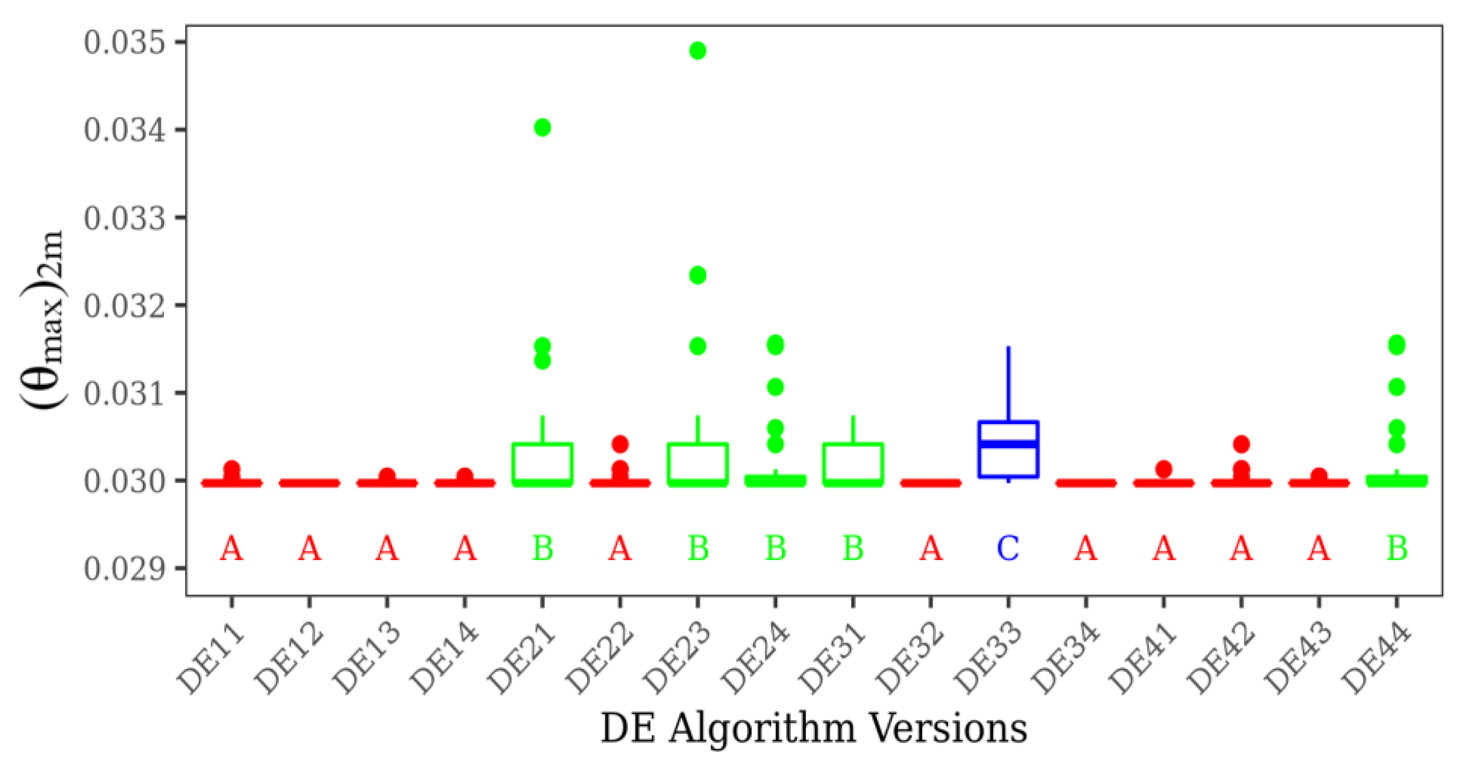
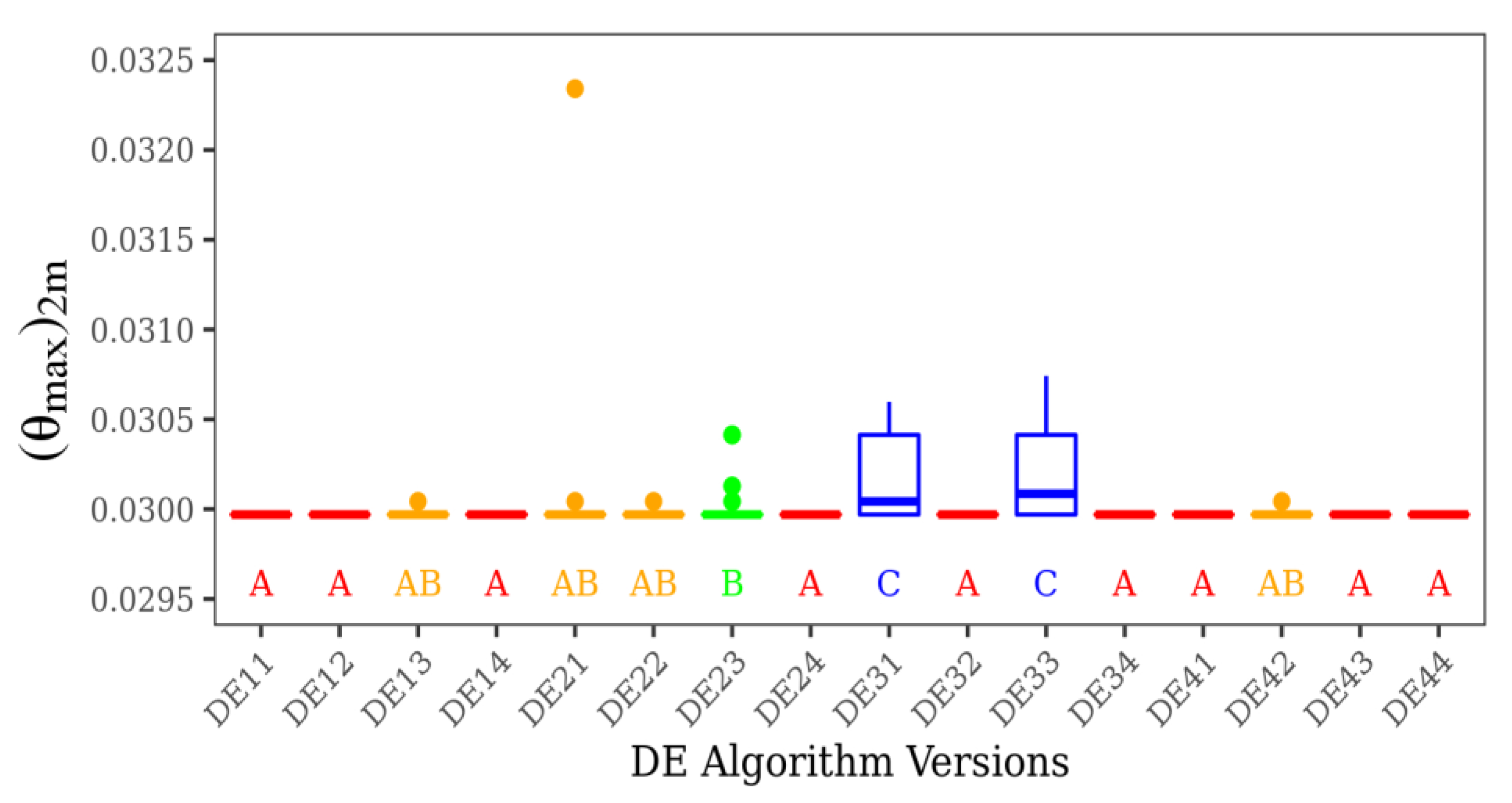
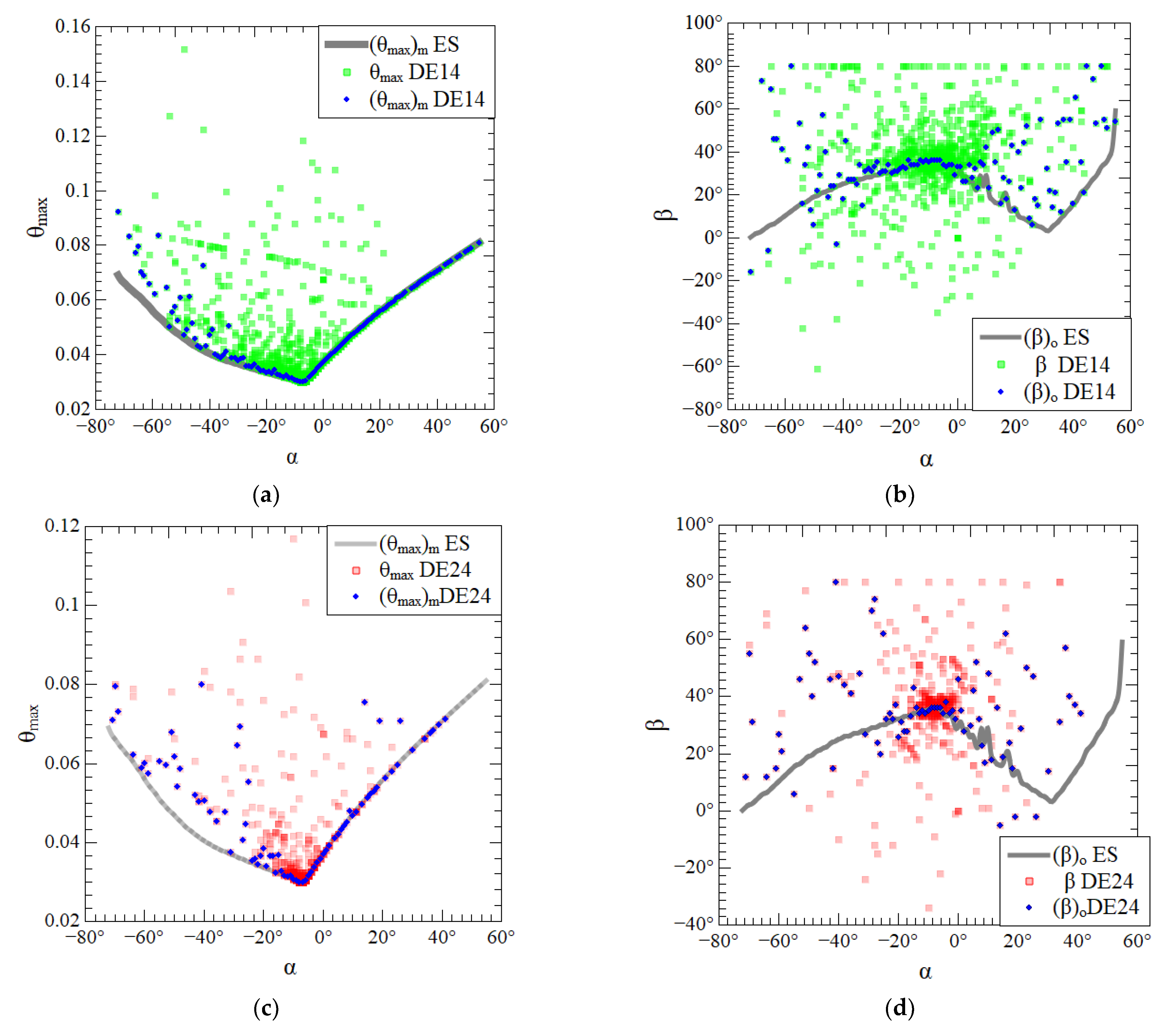
4.2. Optimization Results for Two Degrees of Freedom

For the second level optimization of the double Y-shaped cavity geometry, the algorithms searched for the best angles of (α)_o, and (β)_2o, independently. Two experiments were performed, one with NP = 20 and NG = 50, for all sixteen versions of DE, and a second experiment with NP = 30 and NG = 50.

Table 6. Statistical metrics of the results achieved for achievement of (θ_max)_2m obtained with NP = 20 and NG = 50.

DE Versions	Average (θmax)2m	Variance (× 10−7)	Standard Deviation (×10−5)	RMSE (×10−3)
DE12; DE32; DE34	0.029969	-	-	-
DE13; DE14	0.029974	0.00344	1.86	1.89
DE24; DE44	0.030169	1.94	44.1	47.7
DE33	0.030410	1.66	40.7	59.6
DE21	0.030322	6.53	80.8	86.9
DE23	0.030472	11.2	106.0	115.3

shows the statistical metrics for the first experiment, with NP = 20. The first line of the Table 6 presents the algorithm versions that reached the optimal geometry of (α)_o = −7°, and (β)_2o = 36° for all 30 runs. Therefore, the values of variance, standard deviation, and RMSE are null. The DE versions seem in second line of Table 6 also have a suitable performance (not good as DE12, DE32, and DE34) with low magnitudes of variance, standard deviation and RMSE. In general, the best versions consider the parameter F = 1, except for DE13, that uses F = 1.5. The other algorithms led to a poorer performance in comparison with those of first two lines of Table 6, especially with the increase in the magnitudes of variance, standard deviation, and RMSE.

The impact of the change in population size on the DE algorithm version can be seen in the statistical metrics of

Table 7. Statistical metrics of the results achieved for achievement of (θ_max)_2m obtained with NP = 30 and NG = 50.

DE Versions	Average (θmax)2m	Variance (× 10−8)	Standard Deviation (×10−4)	RMSE (×10−4)
DE11; DE12; DE14; DE24; DE32; DE34; DE41; DE43; DE44	0.029969	-	-	-
DE13; DE22; DE42	0.029972	0.0178	0.134	0.134
DE23	0.030014	1.36	1.17	1.23
DE33	0.030236	7.57	2.75	3.80
DE21	0.030051	18.7	4.33	4.33

. In comparison with the experiment where NP = 20, the population with NP = 30 led to more versions of DE able to reach the optimal geometric configuration on all runs (100%). The worst results continue to emerge from the same versions (DE21, DE23, and DE33). Even with a significant reduction in the variance, standard deviation, and RMSE, the last versions in Table 6 do not reach a similar performance as that achieved for the best codes. The statistical analysis performed by the SW and KW methods validate the significant difference between the investigated algorithm versions. The results of statistical test for both experiments, NP = 20, and NP = 30, are shown in

Table 8. Results of statistical tests for achievement of (θ_max)_2m for DE versions with NP = 20 and NG = 50.

Shapiro–Wilk: Normality Test
DE Versions	p-Value	Distribution
DE12; DE32; DE34	-	Same results for all runs
DE13; DE14	4.402 × 10−11	Non-normal
DE24; ED44	7.169 × 10−9	Non-normal
ED23	1.479 × 10−8	Non-normal
Kruskal–Wallis: Rank Sum Test
DE Versions	p-Value	αs	Differences
DE12–14; DE23, DE24; DE34, DE44	1.576 × 10−8	0.05	Significant
All versions	2.2 × 10−16	0.05	Significant

and

Table 9. Results of statistical tests for achievement of (θ_max)_2m for DE versions with NP = 30 and NG = 50.

Shapiro–Wilk: Normality Test
DE Versions	p-Value	Distribution
DE11, DE12, DE14, DE24, DE32, DE34, DE41, DE43, DE44	-	same results for all runs
DE13, DE22, DE42	7.76 × 10−12	Non-normal
DE33	9.32 × 10−5	Non-normal
ED23	8.97 × 10−12	Non-normal
Kruskal–Wallis: Rank Sum Test
DE Versions	p-Value	αs	Differences
All versions	2.2 × 10−16	0.05	Significant

, respectively. Table 8 and Table 9 show the SW and KW tests for all algorithms and the results presented a non-normal distribution, except those that reached the same magnitude of (θ_max)_2m for all runs.

Figure 6 and Figure 7 show, respectively, the non-parametric multiple comparisons of Dunn tests for the achievement of (θ_max)_2m considering NP = 20 and 30. In Figure 6, three groups were identified by the test of Dunn: A, B and C. Again, group A consists of the algorithms with the best performance, i.e., those where the minimum magnitude of (θ_max)_2m is achieved in almost 100% of the runs, including the algorithms DE12, DE32, and DE34 which obtained the global optimum in all runs. The DE versions in group A have heterogeneous parameters with varied combinations of F, CR, and mutation operators. The algorithms with intermediate performance are classified in group B. Most of the DE versions in this group have the mutation parameter best/1/bin (ED2y) and show high variance. Group C is reserved for the algorithm DE33, which led to the worst performance in terms of achievement of the global point of optimum and variance of results for different runs. In general, the results of Figure 6 indicated that, among the DE versions with rand/1/bin (DE1y), there is no significant difference. For NP = 20 and NG = 50, parameters F and CR do not have significant influence over the optimization performance. However, for the DE2y versions (best/1/bin), the algorithm with parameters F = 1 and CR = 0.7 show a better performance in comparison with others with the same mutation operator.

In Figure 7, it is possible to notice the emergence of an intermediate group, AB, beyond the previous groups seen in Figure 6, which can be a result of the increase in population size from NP = 20 to 30. In Figure 7 it is also notice the predominance of algorithms with the parameter F = 1.0 classified in group A. More precisely, six of nine algorithms with F = 1.0 are in this group. Results also indicated that changes in parameter CR do not lead to significant variations in the performance of different DE versions.

The optimization process performed by the DEx4 versions, groups A and AB, is shown in Figure 8a,b. The optimization evolution of the degree of freedom β is illustrated in the Figure 8a, where it is possible to note the concentration of values near to the optimal angle of (β)_2o = 36°. Figure 8b shows the minimization of the (θ_max)_2m and the convergence to the magnitude (θ_max)_2m = 0.029969. For all versions, it is possible to observe a large spread on the attempts to find the optimal angle β for the first 500 iterations in the range of −60° ≤ (β)_2o ≤ 80°. With the increase in the number of simulations, the algorithms converge to optimal conditions. For the DE41 version, around 1000 iterations are required for convergence of (β)_2o, while D43 is slowly requiring near 1500 iterations for convergence. The fastest algorithms are versions DE42 and DE44, which converge for almost 700 iterations. A similar behavior is noticed in Figure 8b for convergence of the minimum magnitude of (θ_max)_2m. Figure 8 shows that for F = 1, the mutation operators best/1/bin and current-to-best/1/bin have the same behavior.

As previously mentioned, constructal design has its main concern with the comprehension of the effect of the degrees of freedom over the optimal geometry and thermal performance of the flow system. In this sense, Figure 9 shows a comparison of the effect of the degree of freedom α over the once optimized angle β, (β)_o, and the once minimized dimensionless maximum excess of temperature, (θ_max)_m, reached by the exhaustive search (ES) method, in comparison with the results of the differential evolution algorithms. The values registered by meta-heuristics during the search space exploration were ordered according to angle α and can be seen in the points with colors red and green in Figure 9. The effect of α generated by the exhaustive search (ES) method is represented by the gray curve in Figure 9. The blue points in Figure 9 represent the optimal values of (β)_o and minimum magnitudes of (θ_max)_m reached by the meta-heuristics for each value of α. Results for the DE14 version in Figure 9a show that it is possible to reproduce in an approximate form the effect of α over (θ_max)_mfor α > −40°. This behavior occurs due to the slow convergence of the DE14 algorithm version, resulting in scattered data. However, the results of the DE14 in Figure 9b show that this algorithm cannot reproduce the effect of α over (β)_o like the ES method, mainly in the regions near the inferior and superior extremes of the search space of α.

According to Figure 9b, it is possible to obtain an approximation of the effect of α over (β)_o near the optimal region of (α)_o = −7°. For values of α > 0°, the problem has more than one solution when different values of β led to similar values of (θ_max)_m, as can be seen in Figure 9a,c. This behavior happened due to the significant sensitivity of the angle α. For version DE24, the reproduction of the effect of α over (β)_o and (θ_max)_m is more inaccurate due to the fast convergence of the algorithm and the concentration of the exploration in the optimal region of (α)_o, as seen in Figure 9c,d.

Results indicated that different versions of DE were suitable for the prediction of the once minimized magnitude of (θ_max)_m and the corresponding optimal angle β, (β)_o, near the global optimal angle of α. This behavior is indicative that the DE version can be used for the prediction of optimal shapes. Despite that, the reproduction of the effect of one degree of freedom over the performance indicator and corresponding other optimal degrees of freedom is restricted to the global optimum point or limited region of the independent DOF investigated. This aspect should be taken into account in the association between the constructal design and the optimization methods based on computational intelligence.

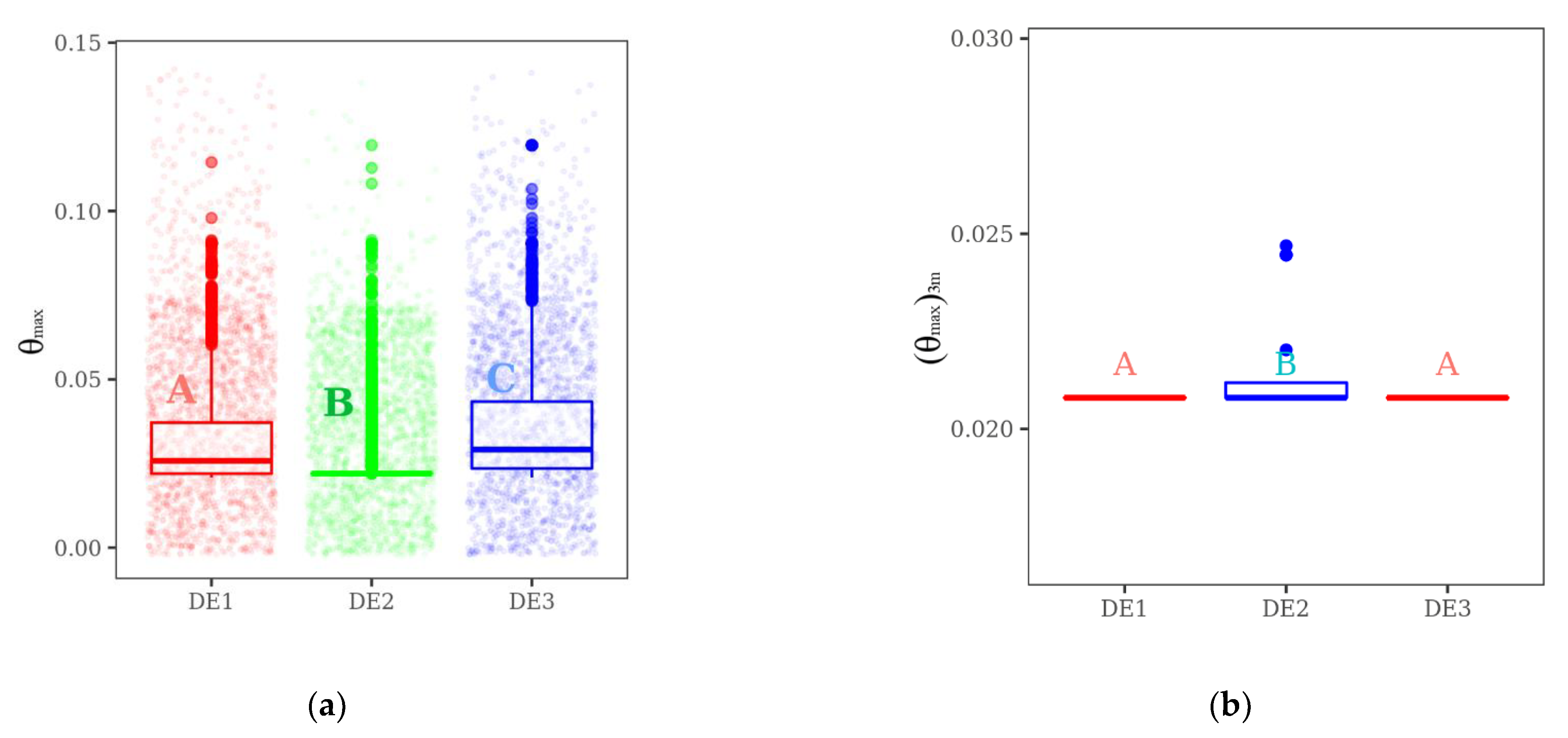
4.3. Optimization Results for Three Degrees of Freedom

Here, it is investigated the optimization of three degrees of freedom, more precisely the ratio S₁/H₀, and the angles α and β. In this investigation, 30 runs are also performed for each version of the DE algorithm. For the height of the inferior branch of the double Y-shaped cavity, represented by rate S₁/H₀, a discrete search space was investigated, S₁/H₀ ∈ [0.1; 0.9] with ∆S₁/H₀ = 0.1. The search space of degrees of freedom α and β was the same as in the previous section. The versions of the DE algorithm used at this level are the ones with better performance in the two degrees of freedom geometric optimization. The amplification factor (F) and crossover rate (CR) parameters are applied with F = 1 and CR = 0.9. The mutation operators investigated are the functions represented by Equations (12), (15) and (16). Therefore, the DE versions are named here as DE1, DE2, and DE3, respectively, according to the mutation operators rand/1/bin, best/1/bin, and best/2/bin. The population size (NP) and the total number of generation (NG) parameters were defined as NP = 30 and NG = 100.

Table 10. Statistical metrics for achievement of (θ_max)_3m for DE versions with NP = 30 and NG = 100.

DE Versions	Average (θmax)3m	Variance	Standard Deviation	Standard Error	RMSE (×10−3)
DE1; DE3	0.020797	0	0	0	0
DE2	0.021520	1.91 × 10−6	1.38 × 10−3	2.52 × 10−4	1.54 × 10−3

shows statistical metrics obtained for different versions of DE algorithms to obtain the three times minimized (θ_max)_3m. More precisely, it presented versions DE1 and DE3 that conducted to the best performance and the version DE2 that conducted to the worst performance. The algorithms DE1 and DE3 also led to the same optimal magnitudes of (S₁/H₀)_o, (α)_2o, and (β)_3o. It is worth mentioning that, even the worst version (DE2) conducted to a similar configuration was found with the best versions of DE.

Table 11. Results of statistical tests for DE versions with NP= 30 and NG =100.

Shapiro–Wilk: Normality Test
DE Versions	p-Value	Distribution
DE1; DE3	-	Same values
DE2	2.018 × 10−8	Non-normal
Kruskal–Wallis: Rank Sum Test
DE Versions	p-Value	αs	Differences
DE1. DE2. DE3	4.42 × 10−6	0.05	Significant

shows the statistical tests of Shapiro–Wilk (SW) and Kruskal–Wallis (KW) for the investigated DE versions. Results seen in Table 11 were calculated from the registry of (θ_max)_3m in the 30 runs of each algorithm. Results of the SW test show that the data do not come from a normal distribution. KW test indicates a significant difference between the DE versions analyzed since the calculated p-value is much smaller than the significance level α_s. Dunn test results were shown in Figure 10, being possible to classify the algorithm versions in groups according to the multiple comparisons, as well as the KW test.

Figure 10 shows the classification of Dunn’s test for the data of exploration of the search space, Figure 10a, and the classification for the convergence to the three times minimized dimensionless maximum excess of temperature, (θ_max)_3m, obtained for the 30 runs of each algorithm, Figure 10b. Points in Figure 10a represent the values of (θ_max)_3m reached by each algorithm during the optimization process of one run. The classification of Dunn’s test indicates that the DE versions have different behaviors in exploring the search space. According to the boxplot and points in Figure 10a, version DE2 has a more concentrated exploration of the search space than other versions, similar to the previous analysis performed in Section 4.2. The concentrated exploration conducted DE2 version to be retained at a local point of minimum. This behavior classifies the DE2 version in group B as different from the other versions, as seen in Figure 10b.

Figure 11 shows the evolution of the optimization process, considering one run for each algorithm, to obtain the three times minimized dimensionless maximum excess of temperature, (θ_max)_3m, and the corresponding optimal geometry, i.e., (S₁/H₀)_o, (α)_2o, and (β)_3o. Figure 11a shows the optimization of (S₁/H₀)_o, being possible to observe that, in general, the DE2 version reached an optimal ratio of (S₁/H₀)_o = 0.9 after almost 1000 simulations. In contrast, other versions of the DE algorithm alternated more, seeking the best configuration, and converged to a value only after 2000 simulations. The convergence velocity of the DE2 version is also observed in Figure 11b–d during the optimization process of (β)_3o, (α)_2o and search for (θ_max)_3m. DE1 algorithm version presents a significant concentration of β values near the optimal value before 1000 simulations but only converged after 2000 simulations, as shown in Figure 11b. DE3 version is the algorithm with more scattered data for the explorations of the β search space with the advancement of simulations. According to the data of Figure 11b, the DE3 version concentrated the results near the optimal configuration of β near the 2000 simulations, converging after this point. For the angle α, Figure 11c shows that the DE2 version reaches the optimal value of (α)_2o = −53° with approximately 750 simulations, i.e., 25 generations. It is also important to observe that, versions DE1 and DE3 did not converge to the optimal (θ_max)_3m for all population individuals. However, these versions have reached the minimum value of (θ_max)_3m for some individuals in the last generations. Slow convergence of these DE versions helps them to escape from the local minimum, explaining the results shown in Table 8 with null variance for all runs of the algorithms. On the other hand, the fast convergence of the DE2 version takes this algorithm to reach some local minimum, as shown in Figure 10b.

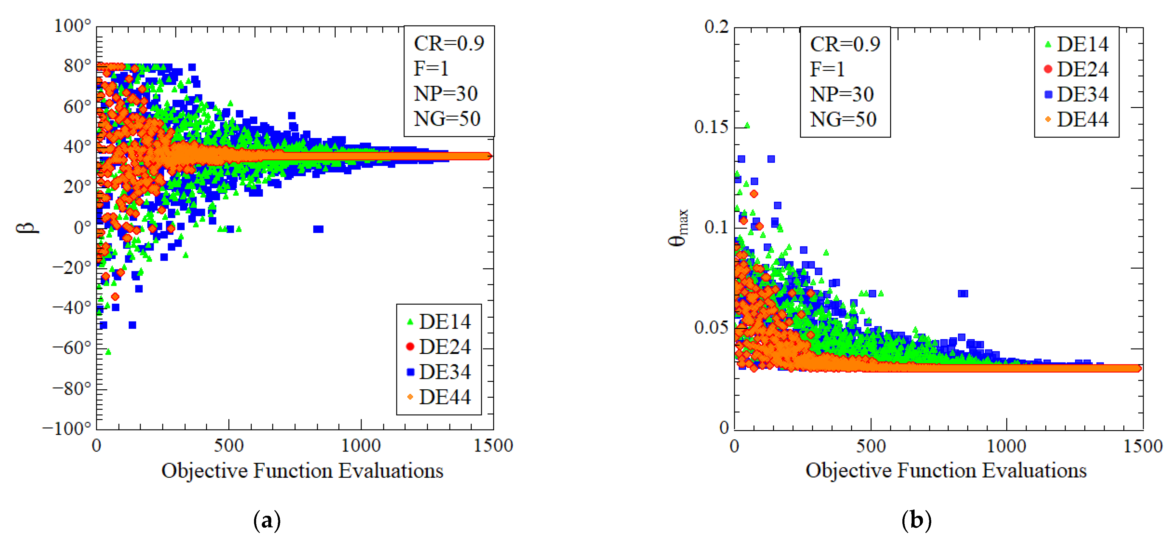
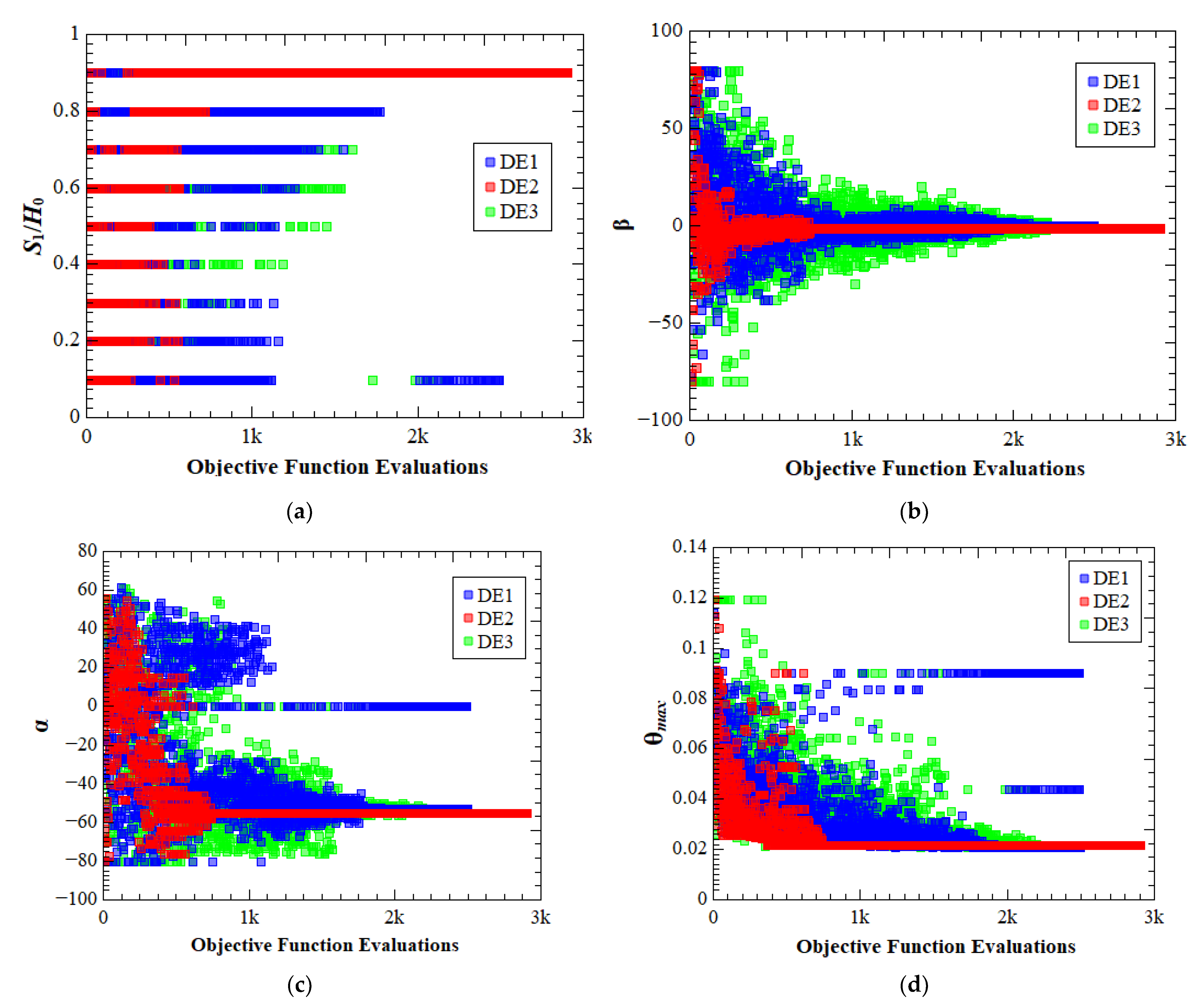
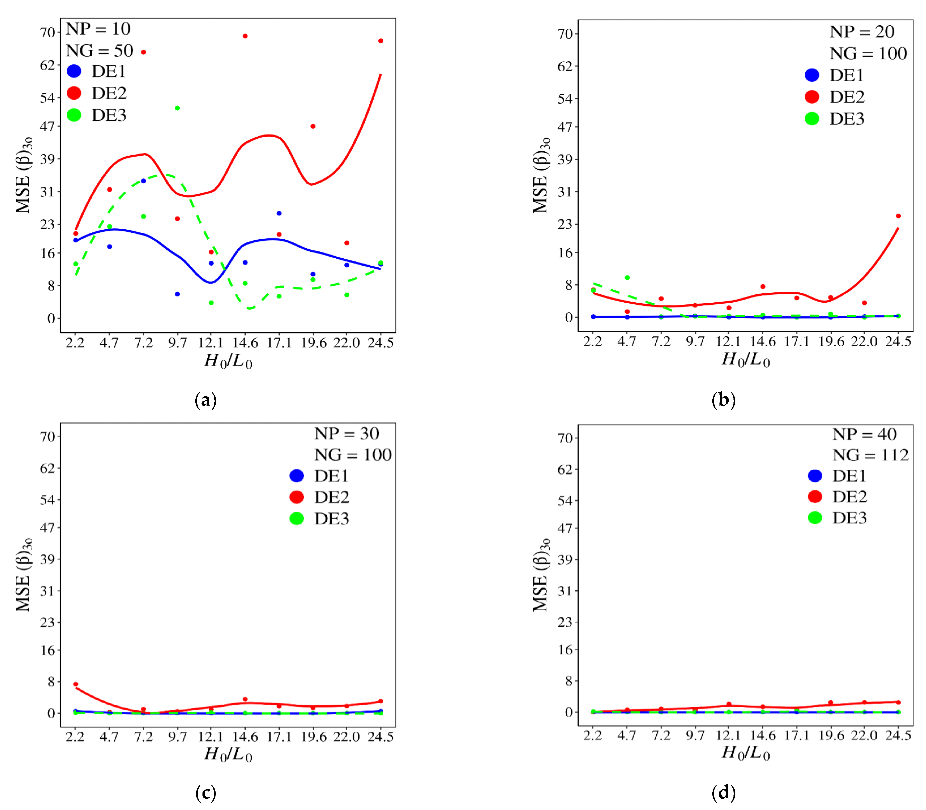
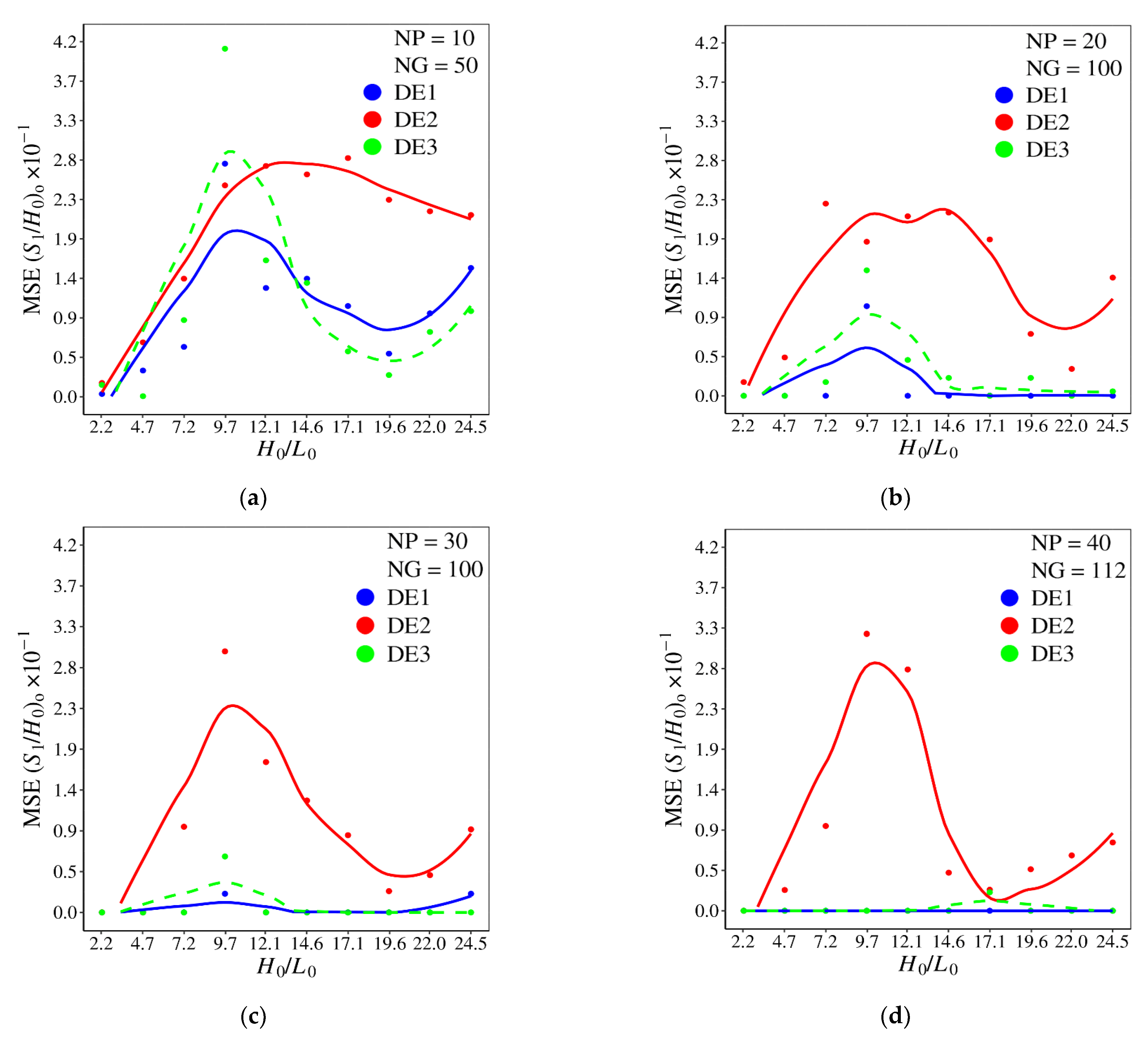
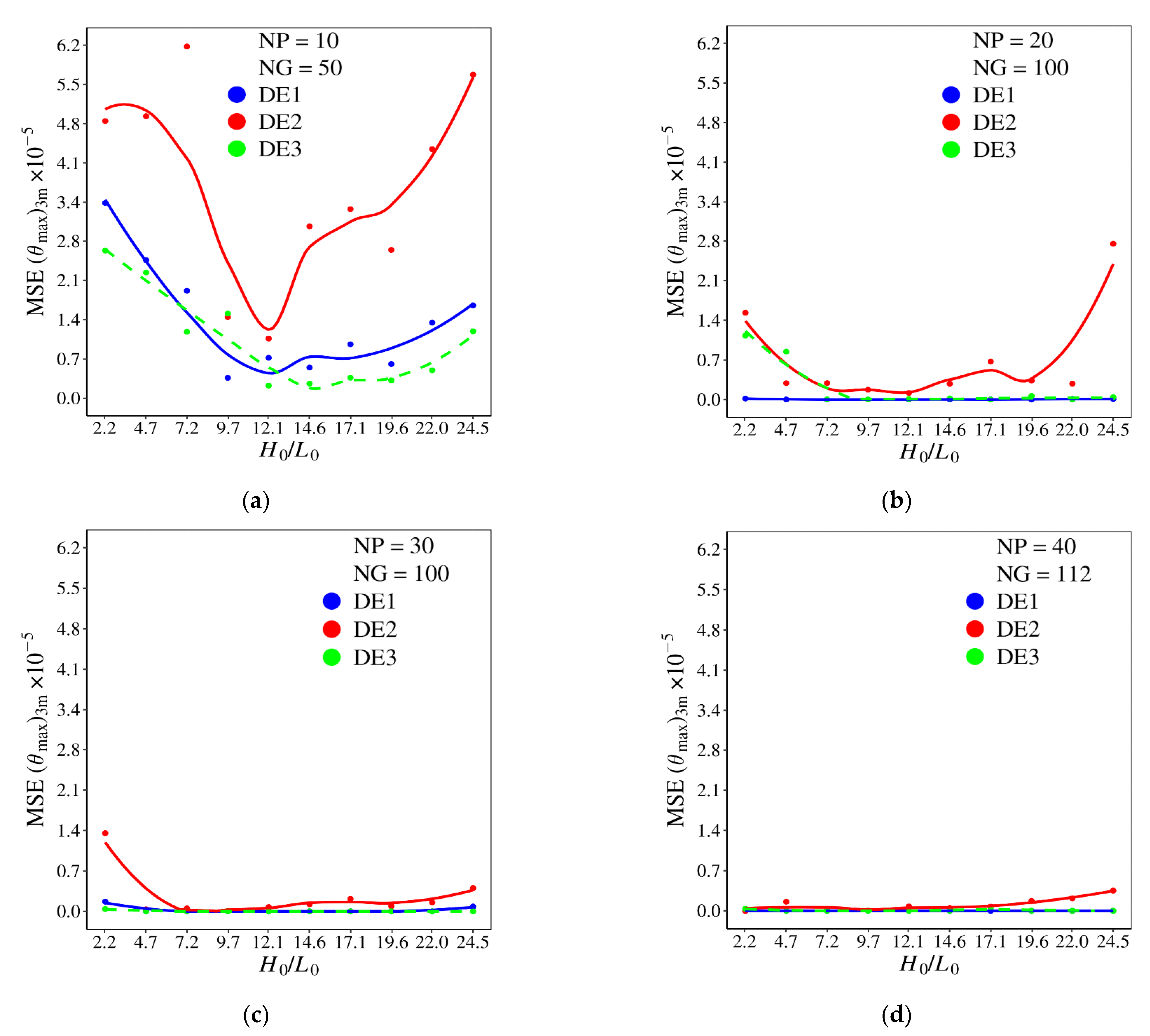
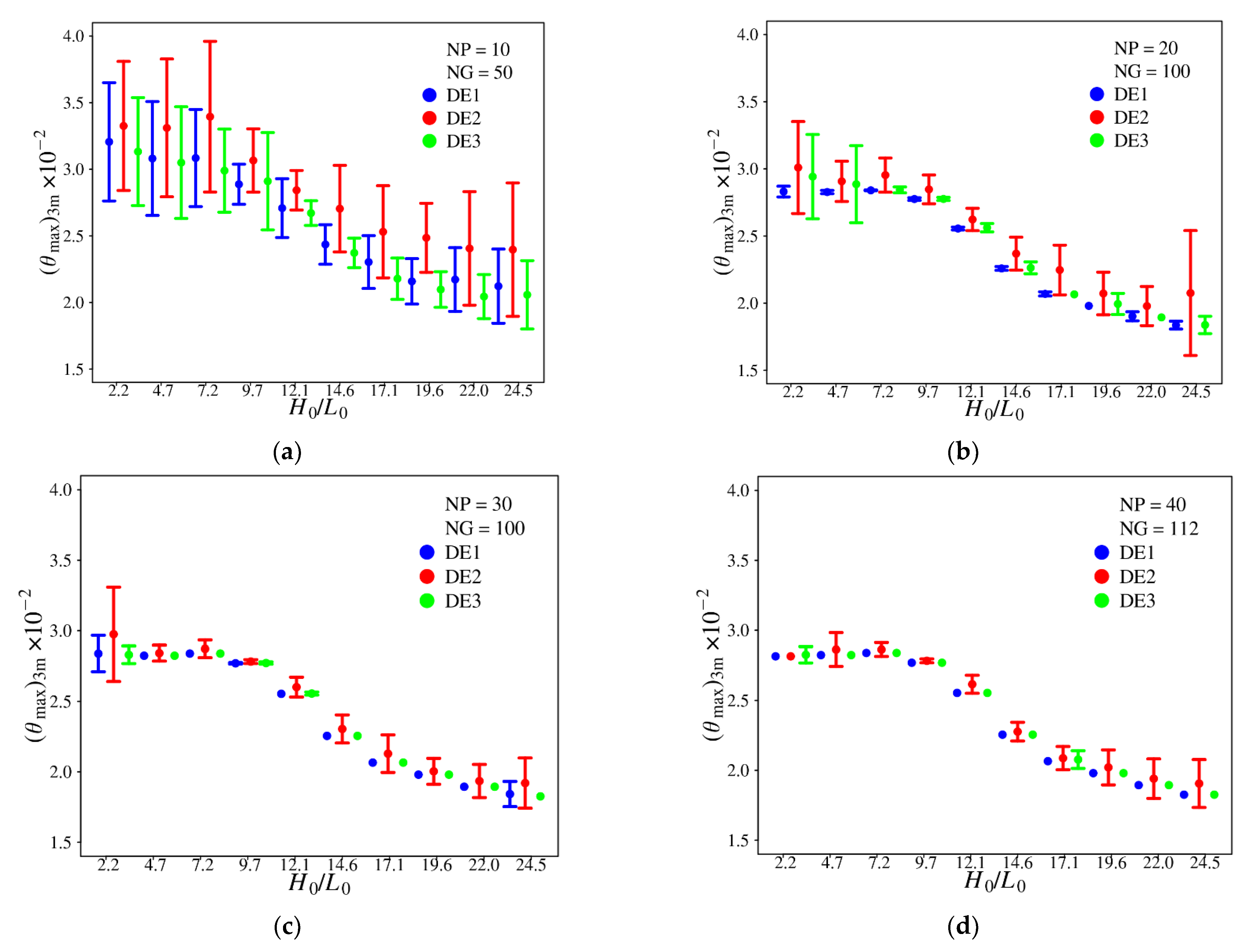
4.4. Optimization Results for Four Degrees of Freedom

In this section, the idea is to reproduce the effect of the ratio H₀/L₀ over the three times minimized maximum excess of temperature, (θ_max)_3m, and the mean square errors (MSE) for (θ_max)_3m and the corresponding optimal configurations, (S₁/H₀)_o, (α)_2o, and (β)_3o, for different versions of DE algorithm. The remaining degrees of freedom and constraints are kept constant, i.e., H/L = 1.0, φ_c = 0.01, and φ₁ = φ₂ =0.015. For geometric optimization it is assumed a discrete search space with α = β ∈ [−80°; 80°] and interval of Δα = Δβ = 1° and S₁/H₀ ∈ [0.1; 0.9] with an interval of ΔS₁/H₀ = 0.1. Based on the previous results, only DE1, DE2, and DE3 with F = 1.0 and CR = 0.0 are used here. An investigation performed here consists of the analysis of the influence of different combinations of the parameters NP and NG over the effect of the ratio H₀/L₀ over the thermal performance and optimal configurations. It executed 30 runs of each algorithm version for the following discrete search space of H₀/L₀:

$$H_0/L_0=\left[ 2.25; 4.72; 7.19; 9.66; 12.14; 14.61; 17.08; 19.55; 22.03;24.5\right]$$

(30)

Table 12. Results of statistical metrics of (θ_max)_3m for some values of H₀/L₀ and different combinations of NP × NG.

		DE1		DE2		DE3
H0/L0	NP × NG	Average (θmax)3m (×10−3)	Standard Deviation (×10−4)	Average (θmax)3m (×10−3)	Standard Deviation (×10−4)	Average (θmax)3m (×10−3)	Standard Deviation (×10−4)
2.25	10 × 50	32.05	44.37	33.25	48.44	31.32	40.51
	20 × 100	28.30	3.99	30.09	34.23	29.42	31.38
	30 × 66	28.39	12.86	29.75	33.39	28.30	6.20
	30 × 100
	40 × 75	28.16	0	28.16	0	28.26	5.81
	40 × 112
12.14	10 × 50	27.08	22.07	28.42	14.84	26.71	9.24
	20 × 100	25.55	1.09	26.23	8.34	25.62	4.43
	30 × 66	25.54	0	26.01	7.04	25.72	3.79
	30 × 100					25.55	1.07
	40 × 75			26.16	6.44	25.57	1.23
	40 × 112					25.54	0
24.50	10 × 50	21.22	27.83	23.96	50.06	20.57	25.65
	20 × 100	18.36	2.93	20.75	46.49	18.37	6.45
	30 × 66	18.45	9.00	19.20	17.84	18.51	5.44
	30 × 100	18.42	8.93			18.26	0
	40 × 75	18.26	0	19.05	17.11	18.30	1.53
	40 × 112					18.26	0

shows the statistical metrics calculated from the results of DE algorithm versions. The first column shows some H₀/L₀ search space values, and the second column shows the combinations of NP × NG investigated. The other columns show the statistical metrics of the average and standard deviation of (θ_max)_3m obtained with DE1, DE2, and DE3 versions. The first combination of NP = 10 and NG = 50 led to the worst results with high magnitudes of standard deviation and overall (θ_max)_3m for all cases of H₀/L₀. These results indicated the achievement of local points of optimum and dispersed magnitudes of thermal performance. In the second experiment, the magnitudes of NP and NG were increased two times (NP = 20 and NG = 100).

Table 12 data indicates a significant improvement in the results, especially in the magnitude of the standard deviation and the decrease in overall (θ_max)_3m close to the global point of (θ_max)_3m. The following experiment tests the population size of 30 individuals and 2 total numbers of generations, 66 and 100. In this case, the results of DE2 and DE3 show some progress. On the other hand, the performance of DE1 for H₀/L₀ = [2.25, 24.5] has a slight decrease. The increase in NG from 66 to 100 does not significantly influence the results, except for the DE3 version in H₀/L₀ = [12.14; 24.5]. For the final experiments with NP = 40 and NG = [75, 112], the DE1 algorithm version showed better results with null values for standard deviation, which means that the algorithm reached the optimal solution in all execution and for all values of rate H₀/L₀. The impact of the increase in NP was expected, but compared to other methods, the DE1 version shows better results even for NP = 20 and NG = 100. The DE2 version also achieved the optimal solution in all executions for H₀/L₀ = 2.25. However, for other values of H₀/L₀, the DE2 version does not reach the optimal solution in all runs. For the DE3 version, the parameters NP = 40 and NG = [75, 112] improved the algorithm results, mainly for NG = 112, with null standard deviation values. Nevertheless, for H₀/L₀ = 2.25, the results slightly decrease compared to NP = 30.

Figure 12 compares the mean square error of α (MSE α) for different combinations of NP × NG and different versions of DE investigated. As expected, in general, the MSE α decreased with the increase in NP and NG parameters. Despite that, in some conditions, the growth of NP and NG parameters does not influence the MSE α, e.g., for the interval 9.7 $\le$ H₀/L₀ $\le$ 12.1 with the DE2 version, a significant decrease in MSE α is not observed, as can be noticed in Figure 12a–d.

For H₀/L₀ $\ge$ 14.6, the decrease in MSE α is more accentuated for DE1 and DE3 versions, mainly for DE1 with NP = 20 and NG = 100. These two algorithm versions had more difficulty obtaining the optimal value of α for H₀/L₀ = 9.7, Figure 12a–c. This behavior indicates that, for this ratio of H₀/L₀, there are more points of local minimal for the prediction of (α)_2o. For NP = 40 and NG = 112, Figure 12d, the algorithms DE1 and DE3 led to MSE α tending to zero, except for H₀/L₀ = 17.1, when DE2 and DE3 have a similar performance.

The mean square error for β (MSE β) for each algorithm version in different NP and NG combinations is shown in Figure 13. For the first combination of NP and NG with NP = 10 and NG = 50, the three algorithm versions analyzed presents several errors for all values of H₀/L₀, Figure 13a. With the increase of the NP and NG parameters, a strong reduction in the magnitude of MSE β was efficiently obtained, as can be seen in Figure 13b–d, mainly for versions DE1 and DE3, which obtained MSE β almost null in all ranges of H₀/L₀ investigated.

It is worth mentioning that, for NP = 20 and NG = 100, Figure 13b, the DE1 version still shows almost zero errors for all ratios of H₀/L₀. Results of Figure 13 show that the DE2 version was not efficient in completely reducing the MSE β for different magnitudes of H₀/L₀. Despite that, the performance was enormously superior to that noticed for the reduction of MSE α, which can be associated with the sensitivity of the ratio H₀/L₀ over (α)_2o and (β)_o.

Figure 14 shows the mean square error for S₁/H₀ (MSE S₁/H₀) as a function of the ratio H₀/L₀ for different versions of DE and magnitudes of NP and NG. The increase in NP and NG led to a decrease in MSE S₁/H₀ in a similar form that happened for MSE α, Figure 12. In other words, the MSE S₁/H₀ had a strong decrease with NP and NG for the versions DE1 and DE3, Figure 14b–d, with more difficulties to reduce the MSE S₁/H₀ for H₀/L₀ < 14.6. The performance of DE2 was not strongly influenced by variation of NP and NG, leading to poor performance, regardless of the magnitude of NP and NG used. It is worth mentioning that the DE1 version shows zero error for all ratios of H₀/L₀ investigated, i.e., the algorithm reaches the optimal values of S₁/H₀ in all runs.

The error to achieve the three times minimized dimensionless maximum excess of temperature, (θ_max)_3m, generated by each DE algorithm version for different ratios of H₀/L₀ and magnitudes of NP and NG is shown in Figure 15. In Figure 15a, the MSE of (θ_max)_3m for NP = 10 and NG = 50 can be seen, showing the highest magnitude errors for the performance indicator, regardless of the DE version used. For the next population size, NP = 20, and total generation of NG = 100, Figure 15b, DE1 version conducted to the minimum error for all ratios of H₀/L₀, which is a strong indicator that this algorithm is able to reproduce the effect of H₀/L₀ over (θ_max)_3m and corresponding optimal configurations, (S₁/H₀)_o, (α)_2o, and (β)_3o, since the search is performed for fixed magnitudes of H₀/L₀ (the curve it is desired to reproduce). For the DE3 version, a similar prediction can be found, but more computational effort is required, since the lowest magnitudes of MSE (θ_max)_3m were obtained with higher values of NP and NG in comparison with DE1. For the DE2 version, the increase in the NP × NG parameters implies a significant reduction in MSE (θ_max)_3m, but still presents the highest errors among the analyzed algorithm, which is an indicative of the prediction of local points of minimum and local optimal configurations.

Figure 16 shows the effect of the ratio H₀/L₀ over (θ_max)_3m considering the overall magnitude, represented by the point, and the inferior and superior limits established by the standard deviation, represented by the bars. The effects of H₀/L₀ on the thermal performance reproduced by different versions of DE and combinations of NP and NG parameters are analyzed. The first experiment with NP = 10 and NG = 50, shown in Figure 16a, presents the highest average and standard deviation values of (θ_max)_3m for all DE algorithm versions and ratios of H₀/L₀. These NP and NG parameters are insufficient to reproduce the effect of H₀/L₀ over (θ_max)_3m for any version of the DE algorithm analyzed. For the next experiment, Figure 16b, with NP = 20 and NP = 100, it is possible to note an improvement in the reproduction of the effect of H₀/L₀ over (θ_max)_3m, mainly for DE1 where low magnitudes of standard deviation are noticed. The DE3 version also has adequate performance, but some magnitudes for overall (θ_max)_3m and standard deviations are higher than those reached with DE1. The performance of the DE versions was improved with the increase in NP and NG up to the configuration with NP = 40 and NG = 112, where the standard deviation for DE1 was null and the global optimal configuration is found for each magnitude of H₀/L₀, reproducing in a most adequate form the effect of H₀/L₀ over (θ_max)_3m. For the present study of the physical problem, the algorithm DE1 with NP = 40 and NG = 112 is highly adequate for the reproduction of the effect of degrees of freedom over the thermal performance and corresponding optimal configurations. As a consequence, it will be used in future studies associated with constructal design for optimization of a complex system with 6 or 7 degrees of freedom, significantly reducing the computational effort in comparison with exhaustive search (benchmark solution).

Figure 17 shows the evolution of the optimal configuration for some values of H₀/L₀, demonstrating the adaptation of the design for different heights of the main stem of a double Y-shaped cavity. Figure 17a–c shows that the optimal values of the (S₁/H₀)_o, (α)_2o, and (β)_3o changed to assume the configurations that led to three times minimized dimensionless maximum excess of temperature (θ_max)_3m in the solid domain for each value of H₀/L₀. In Figure 17c it is possible to notice the configuration that led to the dimensionless maximum excess of temperature four times minimized, (θ_max)_4m, when (H₀/L₀)_o = 24.5. For lower magnitudes of the height of the main stem of the double Y-shaped cavity, Figure 17a, the optimal angles are positive to improve the thermal distribution in the upper region of the solid domain. As the stem height increases, Figure 17b,c, the angles of the branches and the position of the inferior branch are reallocated to redistribute the heat in the center and inferior areas of the solid domain, minimizing the thermal resistance in the solid domain. Figure 17 also demonstrates that the number of hot regions in the solid domain changed from five to six from cases of Figure 17a,b to case Figure 17c, showing that the most homogeneous distribution of temperature leads to the best thermal performance. This behavior is in agreement with the constructal principle of “optimal distribution of imperfections”.

5. Conclusions

The present work analyzed the association between the canonical form of differential evolution (DE) algorithm and the constructal design (CD) for geometrical optimization of a double Y-Shaped cavity inserted in a solid domain with constant heat generation per unit volume. Several parameters of the DE algorithm were investigated to rationalize the search for the global point of optimum design, and mainly for the reproduction of the effect of degrees of freedom over the thermal performance and corresponding optimal configurations, which is essential for the physical analysis of the design. The parameters of the DE algorithm analyzed were the differential amplification factor (F), crossover rate (CR), and four mutation operators (rand/1/bin, best/1/bin, best/2/bin, and current-to-best/1/bin). The combinations of the investigated parameter values generated 16 different versions of the DE algorithm. For statistical analysis of each algorithm at each level of optimization, 30 runs for each version were performed. Results were analyzed with the statistical methods of Shapiro–Wilk, Kruskal–Wallis, and the Dunn test for multiple comparisons for non-parametric samples. With these statistical tools, the work identifies the best and worst sets of DE algorithm parameters when applied to the problem of interest.

In most cases observed, the DE algorithm versions with mutation operator rand/1/bin achieved the best performance, at all different optimization levels. On the other hand, the worst mutation operator was the best/2/bin for the conditions investigated in this study. For constant values of NP and NG, the parameter F significantly influenced the search for the best geometrical configuration. For the present conditions, the CR parameter did not show an important influence. For the first level of optimization, the best parameters to be applied, according to the results of this study, were a combination of parameters F = 1 with CR = 0.9 and the mutations operators rand/1/bin and best/1/bin. Results of the second level of optimization show that for correct reproduction of the effect of a determined degree of freedom over the other geometric parameters and thermal performance, is recommendable an association of the meta-heuristic with the exhaustive search method. In other words, the exhaustive search should be used at the level where the effect of degree of freedom over thermal performance and corresponding optimal shapes is investigated. It was also noticed that versions DE1 and DE3 have similar performance but different behavior to explore the search space. The DE2 version presented more errors and was classified as a different group from other methods. Despite the DE2 version error, it can be seen through the results that this algorithm has a fast convergence to the optimal region. Consequently, in most cases, this version reaches local optimal values. The last experiment carried out here was the optimization process to reproduce the effect of the ratio H₀/L₀ over the three times minimized maximum excess of temperature, (θ_max)_3m, and the mean square errors (MSE) for (θ_max)_3m and the corresponding optimal configurations, (S₁/H₀)_o, (α)_2o, and (β)_3o, for different versions of DE algorithm and parameters NP and NG. Results showed that the increase in parameters NP and NG generally improve the algorithm results, except for some cases of the DE2 version for degrees of freedom α and S₁/H₀. The DE3 version presents a significant reduction of standard deviation with the increase in NP and NG parameters reaching an intermediate performance. The performance of the DE1 version was the best in comparison with the other investigated methods. Even for NP = 20 and NG = 100, the method has obtained very close values to the optimal solutions and almost zero standard deviation. The DE1 method required lower computational effort than the DE2 and DE3 methods to sufficiently reproduce the effect of H₀/L₀ over (θ_max)_3m and the corresponding optimal geometries. In general, results indicated that the use of the DE algorithm can be associated with constructal design for prediction on the effect of the influence of different degrees of freedom over the thermal performance and corresponding optimal shapes with a computational effort significantly reduced in comparison with the exhaustive search. Therefore, for future studies, a complete optimization (with 6 or 7 degrees of freedom) of the double Y-shaped cavity will be performed.

References

1. Bejan, A. Constructal-theory network of conducting paths for cooling a heat generating volume. Int. J. Heat Mass Transf. 1997, 40, 799–816. [Google Scholar] [CrossRef]
2. Bejan, A. Freedom and Evolution: Hierarchy in Nature, Society and Science; Springer International Publishing: Cham, Switzerland, 2020; ISBN 978-3-030-34008-7. [Google Scholar]
3. Bejan, A. Shape and Structure, from Engineering to Nature; Cambridge University Press: Cambridge, UK, 2000. [Google Scholar]
4. Dos Santos, E.D.; Isoldi, L.A.; Gomes, M.D.N.; Rocha, L.A.O. The Constructal Design Applied to Renewable Energy Systems. In Sustainable Energy Technologies; Rincón-Mejía, E., de las Heras, A., Eds.; CRC Press: Boca Raton, FL, USA, 2017; pp. 45–62. ISBN 978-1-315-26997-9. [Google Scholar]
5. Rocha, L.A.O.; Lorente, S.; Bejan, A. Constructal Theory in Heat Transfer. In Handbook of Thermal Science and Engineering, 1st ed.; Springer International Publishing: Cham, Switzerland, 2017; pp. 1–32. [Google Scholar] [CrossRef]
6. Gonzales, G.V.; Lorenzini, G.; Isoldi, L.A.; Rocha, L.A.O.; Dos Santos, E.D.; Neto, A.S. Constructal Design and Simulated Annealing applied to the geometric optimization of an isothermal Double T-shaped cavity. Int. J. Heat Mass Transf. 2021, 174, 121268. [Google Scholar] [CrossRef]
7. Biserni, C.; Rocha, L.A.O.; Bejan, A. Inverted fins: Geometric optimization of the intrusion into a conducting wall. Int. J. Heat Mass Transf. 2004, 47, 2577–2586. [Google Scholar] [CrossRef]
8. Biserni, C.; Rocha, L.A.O.; Stanescu, G.; Lorenzini, E. Constructal H-shaped cavities according to Bejan’s theory. Int. J. Heat Mass Transf. 2007, 50, 2132–2138. [Google Scholar] [CrossRef]
9. Xie, Z.; Chen, L.; Sun, F. Geometry optimization of T-shaped cavities according to constructal theory. Math. Comput. Model. 2010, 52, 1538–1546. [Google Scholar] [CrossRef]
10. Lorenzini, G.; Biserni, C.; Isoldi, L.A.; dos Santos, E.D.; Rocha, L.A.O. Constructal Design applied to the geometric optimization of Y-shaped cavities embedded in a conducting medium. ASME-J. Electron. Packag. 2011, 133, 041008. [Google Scholar] [CrossRef]
11. Lorenzini, G.; Biserni, C.; Rocha, L.A.O. Geometric optimization of X-shaped cavities and pathways according to Bejan’s theory: Comparative analysis. Int. J. Heat Mass Transf. 2014, 73, 1–8. [Google Scholar] [CrossRef]
12. Hajmohammadi, M.R. Introducing a ψ-shaped cavity for cooling a heat generating medium. Int. J. Therm. Sci. 2017, 121, 204–212. [Google Scholar] [CrossRef]
13. Hajmohammadi, M.R. Optimal design of tree-shaped inverted fins. Int. J. Heat Mass Transf. 2018, 116, 1352–1360. [Google Scholar] [CrossRef]
14. Lorenzini, G.; Biserni, C.; da Silva Diaz Estrada, E.; Domingues Dos Santos, E.; André Isoldi, L.; Oliveira Rocha, L.A. Genetic Algorithm Applied to Geometric Optimization of Isothermal Y-Shaped Cavities. J. Electron. Packag. 2014, 136, 031011. [Google Scholar] [CrossRef]
15. Lorenzini, G.; Biserni, C.; Estrada, E.D.; Isoldi, L.A.; Dos Santos, E.D.; Rocha, L.A.O. Constructal Design of Convective Y-Shaped Cavities by Means of Genetic Algorithm. J. Heat Transf. 2014, 136, 071702. [Google Scholar] [CrossRef]
16. Gonzales, G.V.; da SDEstrada, E.; Emmendorfer, L.R.; Isoldi, L.A.; Xie, G.; Rocha LA, O.; Dos Santos, E.D. A comparison of simulated annealing schedules for constructal design of complex cavities intruded into conductive walls with internal heat generation. Energy 2015, 93, 372–382. [Google Scholar] [CrossRef]
17. Gonzales, G.V.; Dos Santos, E.D.; Isoldi, L.A.; Rocha, L.A.O.; Silva Neto, A.J.; Telles, W.R. Constructal Design of Double T-shaped cavity with stochastic methods Luus-Jaakola and Simulated Annealing. Defect Diffus. Forum 2017, 370, 152–161. [Google Scholar] [CrossRef]
18. Gonzales, G.V.; Isoldi, L.A.; Rocha, L.A.O.; Silva Neto, A.J.; Dos Santos, E.D. Evaluation of a differential evolution/constructal design algorithm for geometrical optimization of double T-shaped cavity intruded into a heat generating wall. Defect Diffus. Forum 2019, 396, 145–154. [Google Scholar] [CrossRef]
19. Fagundes, T.M.; Lorenzini, G.; Estrada, E.D.S.; Isoldi, L.A.; Dos Santos, E.D.; Rocha, L.A.O.; da Silva Neto, A.J. Constructal Design of Conductive Asymmetric Tri-Forked Pathways. J. Eng. Thermophys. 2019, 28, 26–42. [Google Scholar] [CrossRef]
20. Echevarría, L.C.; Santiago, O.L.; Fajardo, J.A.H.; Silva Neto, A.J.; Sánchez, D.J. A variant of the particle swarm optimization for the improvement of fault diagnosis in industrial systems via faults estimation. Eng. Appl. Artif. Intell. 2012, 28, 36–51. [Google Scholar] [CrossRef]
21. Platt, G.M.; Lima, L.V.P.D.C. Azeotropy in a refrigerant system: A useful scenario to test and compare metaheuristics. Int. J. Metaheuristics 2018, 7, 43. [Google Scholar] [CrossRef]
22. De-La-Cruz-Martinez, S.J.; Mezura-Montes, E. Boundary Constraint-Handling Methods in Differential Evolution for Mechanical Design Optimization. In Proceedings of the 2020 IEEE Congress on Evolutionary Computation, CEC 2020, Glasgow, UK, 19–24 July 2020. [Google Scholar]
23. Özisik, M.N. Heat Conduction, 2nd ed.; John Wiley and Sons Inc.: Raleigh, NC, USA, 1993. [Google Scholar]
24. Reddy, J.N.; Gartling, D.K. The Finite Element Method in Heat Transfer and Fluid Dynamics; McGrawHill: New York, NY, USA, 1994. [Google Scholar]
25. MATLAB. Partial Differential Equation Toolbox User’s Guide R2018b; The MathWorks, Inc.: Natick, MA, USA, 2018. [Google Scholar]
26. Storn, R.; Price, K. Differential Evolution—A Simple and Efficient Heuristic for Global Optimization over Continuous Spaces. J. Glob. Optim. 1997, 11, 341–359. [Google Scholar] [CrossRef]
27. R Core TEAM. R: A language and environment for statistical computing. In R Foundation for Statistical Computing; R Core Team: Vienna, Austria, 2021. [Google Scholar]
28. Shapiro, A.S.S.; Wilk, M.B. An Analysis of Variance Test for Normality (Complete Samples). Biom. Trust 1965, 52, 591–611. [Google Scholar] [CrossRef]
29. Kruskal, W.H.; Wallis, W.A. Use of ranks in one-criterion variance analysis stable. J. Am. Stat. Assoc. 1952, 47, 583–621. [Google Scholar] [CrossRef]
30. Dunn, O.J. Multiple Comparisons Using Rank Sums. Technometrics 1964, 6, 241–252. [Google Scholar] [CrossRef]
Figure 1. Computational domain of the double Y-shaped cavity.
Applsci 13 01998 g001
Figure 2. Triangular mesh used by FEM from MATLAB® PDE toolbox: (a) coarse mesh with 1250 triangular elements; (b) symmetric half of the domain numerically solved during optimization process with a fine mesh of triangular elements.
Applsci 13 01998 g002
Figure 3. Flowchart of the DE algorithm applied to double Y-shaped cavity geometric optimization.
Applsci 13 01998 g003
Figure 4. Dunn test of some DE versions for achievement of (θmax)m.
Applsci 13 01998 g004
Figure 5. Dunn test of all DE versions studied for achievement of (θmax)m.
Applsci 13 01998 g005
Figure 6. Dunn test of all DE versions for (θmax)2m with NP = 20 and NG = 50.
Applsci 13 01998 g006
Figure 7. Dunn test of all DE versions for (θmax)2m with NP = 30 and NG = 50.
Applsci 13 01998 g007
Figure 8. Optimization process of DEx4 versions with NP = 30 and NG = 50: (a) optimization of (β)2o; (b) minimization of (θmax)2m.
Applsci 13 01998 g008
Figure 9. Comparison between the effect of α over (θmax)m and (β)o generated with exhaustive search and the exploration of the search space with differential evolution algorithms: (a) effect of α over (θmax); (b) effect of α over (β)o; (c) effect of α over (θmax); (d) effect of α over (β)o.
Applsci 13 01998 g009
Figure 10. Results of the Dunn’s test for minimization of (θmax)3m optimization of tree degrees of freedom: (a) search space exploration of DE versions for one run; (b) results for thirty runs of each algorithm version.
Applsci 13 01998 g010
Figure 11. Search space exploration with differential evolution algorithms for the three times optimized configuration: (a) (S1/H0)o, (b) (β)3o, (c) (α)2o (d) (θmax)3m.
Applsci 13 01998 g011
Figure 12. Effect of H0/L0 over mean square error (MSE) of α for different DE versions and combinations of NP × NG: (a) NP = 10, NG = 50; (b) NP = 20, NG = 100; (c) NP = 30, NG = 100; (d) NP = 40, NG = 112.
Applsci 13 01998 g012
Figure 13. Effect of H0/L0 over mean square error (MSE) of β for different DE versions and combinations of NP × NG: (a) NP = 10, NG = 50; (b) NP = 20, NG = 100; (c) NP = 30, NG = 100; (d) NP = 40, NG = 112.
Applsci 13 01998 g013
Figure 14. Effect of H0/L0 over mean square error (MSE) of S1/H0 for different DE versions and combinations of NP × NG: (a) NP = 10, NG = 50; (b) NP = 20, NG = 100; (c) NP = 30, NG = 100; (d) NP = 40, NG = 112.
Applsci 13 01998 g014
Figure 15. Effect of H0/L0 over mean square error (MSE) of (θmax)3m for different DE versions and combinations of NP × NG: (a) NP = 10, NG = 50; (b) NP = 20, NG = 100; (c) NP = 30, NG = 100; (d) NP = 40, NG = 112.
Applsci 13 01998 g015
Figure 16. Effect of H0/L0 over overall (θmax)3m and standard deviation for different DE versions and combinations of NP × NG: (a) NP = 10, NG = 50; (b) NP = 20, NG = 100; (c) NP = 30, NG = 100; (d) NP = 40, NG = 112.
Applsci 13 01998 g016
Figure 17. Optimal geometries for different values of H0/L0: (a) H0/L0 = 2.25, (S1/H0)o = 0.1, (α)2o = 43°, (β)3o = 72°, (θmax)3m = 0.0281; (b) H0/L0 = 12.14, (S1/H0)o = 0.9, (α)2o = −45°, (β)3o = 27°, (θmax)3m = 0.0255; (c) (H0/L0)o = 24.5, (S1/H0)2o = 0.9, (α)3o = −62°, (β)4o = −29°, (θmax)4m = 0.0186.
Applsci 13 01998 g017