Kernel Density Derivative Estimation of Euler Solutions

Abstract

Conventional Euler deconvolution is widely used for interpreting profile, grid, and ungridded potential field data. The Tensor Euler deconvolution applies additional constraints to the Euler solution using all gravity vectors and the full gravity gradient tensor. These algorithms use a series of different-sized moving windows to yield many solutions that can be employed to estimate the source location from the entire survey area. However, traditional discrimination techniques ignore the interrelation among the Euler solutions, so they cannot be employed to separate adjacent targets. To overcome this difficulty, we introduced multivariate Kernel Density Derivative Estimation (KDDE) as an extension of Kernel Density Estimation, which is a mathematical process to estimate the probability density function of a random variable. The multivariate KDDE was tested on a single cube model, a single cylinder model, and three composite models consisting of two cubes with various separations using gridded data. The probability value calculated by the multivariate KDDE was used to discriminate spurious solutions from the Euler solution dataset and isolate adjacent geological sources. The method was then applied to airborne gravity data from British Columbia, Canada. Then, the results of synthetic models and field data show that the proposed method can successfully locate meaningful geological targets.

1. Introduction

The studies on the edges of geological bodies are significant for potential field data interpretation. Furthermore, when studying lateral inhomogeneity, especially the position of the edges of anomalous sources, gravity and magnetic surveys have advantages for detecting geological structures like faults and tectonic boundaries [1]. With the development of gravity gradient measurement methods and corresponding interpretation techniques, many edge-enhancement techniques have been proposed in recent years, such as edge detection [2], total variation [3], edge-preserved inversion [4], and focusing inversion [5]. Gravity gradient measurements are a multicomponent gradiometric surveying technology that measures different components of Full Tensor Gravity (FTG) data and have been widely carried out and have yielded large amounts of high-precision FTG data. However, FTG data impose higher requirements on their corresponding interpretation techniques because they often generate more complex anomalies for given sources [6].

Compared with other interpretation techniques of FTG data, Euler deconvolution is suitable for analyzing and interpreting large-area potential field data because it does not rely on prior geological information [7,8]. Euler deconvolution is based on the Euler homogeneity relationship and uses a moving window to traverse potential field data to determine locations and structural indices (SIs) of geological targets [9,10,11,12,13,14,15,16,17,18]. The SIs are associated with the source geometry [19,20,21] and need to be determined in advance for performing Euler deconvolution [22]. Nevertheless, the use of a single structural index (N) makes it difficult to characterize multiple anomaly sources [22,23,24,25,26].

Many extended Euler deconvolution methods have been presented to reduce the influence of the SIs [27,28,29,30,31]. However, traditional Euler deconvolution produces spurious solutions possibly because of noise, either natural or due to the fast Fourier transform (FFT) [32,33,34,35,36]. To overcome this difficulty, various methods have been proposed to optimize the determination of SIs [37,38,39,40,41], many extended Euler deconvolution methods are proposed to eliminate the dependence on predicted N [23,42,43,44,45,46,47], and several methods have been proposed to filter out spurious solutions [17,30,34,35]. For example, Gerovska and Araúzo-Bravo [14] eliminated spurious solutions using the differential similarity transformation based on the error estimations of singular point coordinates and SIs. Yao et al. [48] proposed a horizontal gradient filtering criterion for removing solutions with a small horizontal gradient modulus, a distance constraint criterion for rejecting solutions far from their corresponding moving windows, and a constraint criterion for eliminating solutions with low convergence. Reid et al. [30] filtered spurious solutions according to their clustering, misfit, and the depth and distance from the moving window.

Euler deconvolution with the correct predicted N yields a tight cluster, which is formed by Euler solutions [19,25,49]. Mikhailov et al. [50] developed a clustering technique based on artificial intelligence to select reliable Euler solutions. However, clustering methods cannot discriminate spurious solutions efficiently in shallow sources and neighboring bodies [50,51]. FitzGerald et al. [34] reported spurious solution rejection using skewness and kurtosis obtained by histogram; however, it was difficult to correct for multiple anomalous sources. The density histogram was employed to visualize each formation to check the coherency of the inversion process [52]; however, it was difficult to efficiently divide a multi-dimensional space into non-coherent histogram bins to keep the error rates small [53]. A probability density distribution is a continuous version of a histogram with density and is widely used in geophysical inversions. Such as, Rayleigh wave inversion [54], electromagnetic inversion [55], gravity inversion [56], and joint inversion of gravity and magnetic data [57,58,59,60].

Unlike the histogram, Kernel density estimation (KDE) produces smooth probability density distributions, indicating multimodality more convincingly. The deviation of the kernel estimator is one order of magnitude greater than that of the histogram estimator [61]. The KDE is a nonparametric method for estimating the probability density function of a random variable [62]. It can reject sparsely located solutions and retain dense clusters formed by compact Euler solutions. Moreover, KDE lays a solid foundation for density-based clustering algorithms, which are based on the idea that objects forming dense regions should be grouped into a cluster [63,64]. Ugalde and Morris [65] applied KDE to filter spurious solutions; then, a fuzzy c-means clustering algorithm (FCM) was employed in the filtered data set to locate anomalous sources. Michel [66] used KDE to estimate the relationship between data and predictions from geophysical 1D inversions. The former can be applied when the relationship deviates from linear and Gaussian assumptions. Eckert-Gallup and Martin [67] employed bivariate KDE for generating the joint probability distribution of significant wave height and energy period.

Traditional discrimination techniques use markers with different shapes, colors, or/and sizes to indicate depth and SI values for Euler solutions for locating anomalous sources [33,68,69]. However, these methods can hardly analyze complex Euler solution datasets. Furthermore, traditional discrimination techniques cannot evaluate the overall quality of the solutions or determine how dense/compact the clusters are [34,65], such as dense distributions (for example, the centroids of geological bodies) and sparse distributions, for example, the gaps among geological bodies, of Euler solutions. The multivariate Kernel Density Derivative Estimation (KDDE), extended from KDE, can be used to determine density clusters and distributions for given sample data [70]. Non-parametric statistical techniques, such as KDE and KDDE, have higher computational requirements because they need to evaluate joint probability density distributions on a multi-dimensional domain. Both KDDE and KDE can be considered a convolution, which can be quickly implemented using a FFT [71,72].

The tensor Euler deconvolution converges faster [33,73] and produces tighter clusters than traditional Euler deconvolution [74]. Therefore, we obtained Euler solutions from tensor Euler deconvolution of FTG data for coordinates x_o, y_o, z_o, and N. Then, we used multivariate KDDE with a comparative analysis process to obtain probability density curves, images, and isosurfaces for various combinations of elements of Euler solutions x_o, y_o, z_o, and N, such as {x_o}, {x_o, z_o}, {x_o, z_o, N}, and {x_o, y_o, z_o, N}. The results of synthetic models and field data show that probability density isosurfaces effectively discriminate spurious solutions and isolate complex geological sources.

2. Materials and Methods

2.1. Tensor Euler Deconvolution

Euler deconvolution is a semi-automatic/automatic interpretation method based on Euler’s homogeneity equation, and it has been widely used to interpret profile, grid, and ungridded potential field data. The higher-order differentiation of gravitational potential is the homogenous function in Euler’s sense. The tensor Euler deconvolution equation is composed of two similar Equations (1) and (2) and the traditional Euler Equation (3):

$$x_o\frac{\partial g_x}{\partial x}+y_o\frac{\partial g_x}{\partial y}+z_o\frac{\partial g_x}{\partial z}-N\left(B_x-g_x\right)=x\frac{\partial g_x}{\partial x}+y\frac{\partial g_x}{\partial y}+z\frac{\partial g_x}{\partial z}+{\gamma }_x$$

(1)

$$x_o\frac{\partial g_y}{\partial x}+y_o\frac{\partial g_y}{\partial y}+z_o\frac{\partial g_y}{\partial z}-N\left(B_y-g_y\right)=x\frac{\partial g_y}{\partial x}+y\frac{\partial g_y}{\partial y}+z\frac{\partial g_y}{\partial z}+{\gamma }_y$$

(2)

$$x_o\frac{\partial g_z}{\partial x}+y_o\frac{\partial g_z}{\partial y}+z_o\frac{\partial g_z}{\partial z}-N\left(B_z-g_z\right)=x\frac{\partial g_z}{\partial x}+y\frac{\partial g_z}{\partial y}+z\frac{\partial g_z}{\partial z}+{\gamma }_z$$

(3)

where (x, y, z) are the coordinates of the observation points; (x_o, y_o, z_o) is the location of the source; $g_x$, $g_y$, $g_z$ are the components of the gravity vector; for all pairs $\left(\alpha ,\beta \right)$ in $\left\{x,y,z\right\}$, $g_{\alpha \beta }$ represents a component of FTG, which is obtained by analytical solutions, or a FFT; the structural index N depends on the source geometry; the parameter $B_{\alpha }$ is simply the background, or regional field [33]; ${\gamma }_{\alpha }$ is a constant that usually vanishes except for N = 0 [65]. The N defining the geometry of the anomalous source needs to be determined in advance [22,38]. However, the use of a single N makes it difficult to characterize multiple anomaly sources [22,23,24,25,26]. Traditional Euler deconvolution uses a series of predefined SIs and yields many spurious solutions. Alternatively, using tentative SIs makes Euler deconvolution subjective and time-consuming because the interpreter/user must evaluate the quality of clusters of Euler solutions as the SIs change [19]. To overcome these problems, N will not be predicted [14,34,35].

Tensor Euler deconvolution uses a moving window (length × width = $w_x$ × $w_y$) with $w_n$ observation points to traverse gridded potential field data. Then, each window location generates a solution consisting of the causative source’s location (x_o, y_o, z_o) and N. For the ith moving window, Equations (1)–(3) are rewritten in matrix form as follows:

$$Am=b$$

(4)

where $A={\left[A_1, \dots ,A_l, \dots ,A_{w_n}\right]}^T$, $A_l=[{\left(\partial g_{\alpha }/\partial x\right)}_l,{\left(\partial g_{\alpha }/\partial y\right)}_l,{\left(\partial g_{\alpha }/\partial z\right)}_l,$ ${\left(g_{\alpha }-B_{\alpha }\right)}_l]$, $b={[b_1,}^{}$ ${\dots ,b_l, \dots ,b_{w_n}]}^T$, and $b_l={\left(x\partial g_{\alpha }/\partial x\right)}_l+{\left(y\partial g_{\alpha }/\partial y\right)}_l+$ ${\left(z\partial g_{\alpha }/\partial z\right)}_l$. The subscript l represents the sequence number of the moving sliding window, $m$ represents the Euler solution datasets $\left\{x_o,y_o,z_o,N\right\}$, and $m_i$ is the ith Euler solution written as $[x_o^i,y_o^i,z_o^i,N^i]$.

2.2. Multivariate KDDE of the Euler Solution Datasets

Multivariate KDDE is considered a nonparametric approach for calculating probability density distributions of data instances. Nonparametric approaches have the advantages of asymptotic unbiasedness, square consistency, and uniform convergence. Multivariate KDDE is a trendy tool for analyzing low-dimensional data instances [75,76]. Letting $X=\left(X_1, \dots ,X_i, \dots ,X_n\right)$ be a d-dimensional random sample drawn from a density function $F$, the general form of a multivariate kernel density estimator at any given estimation point $x=\left(x_1,\cdots ,x_d\right)$ can be defined as follows [77]:

$$\overline{F}(x;H)={\displaystyle {\sum }_{i=1}^n{K}_H\left(x-X_i\right)}$$

(5)

where $H$ is a symmetric positive definite $d\times d$ diagonal bandwidth matrix; the multivariate kernel function $K_H\left(x\right)=n^{-1}{\left|H\right|}^{-1/2}K\left(H^{-1/2}x\right)$ is the inner product of the scaled kernel, which is a rescaling of the unscaled kernel $K$ by the bandwidth matrix $H$ [62]; $\left|H\right|$ is the matrix determinant of $H$ and $H^{-1/2}$ is the inverse square root of its matrix. $X_i=\left(X_{i1},\cdots ,X_{id}\right)$ is the various combinations of the elements of Euler solutions, such as $x_o^{}$, $\left(x_o^{},z_o^{}\right)$, $\left(x_o^{},z_o^{},N\right)$, and $\left(x_o^{},y_o^{},z_o^{},N\right)$. Hence, in this paper, $1\le d\le 4$.

Traditional discrimination techniques cannot evaluate the overall quality of the solutions or determine how dense/compact the clusters are [65]. There is no difference between sparse and dense distributions of Euler solutions in a scatter plot drawn by traditional discrimination techniques. Crucial information about the potential density structure fails to be recovered using density estimation results, such as saddles, peaks, and valleys. In contrast, the density derivative estimation effectively overcomes this problem. Therefore, taking the partial derivative of Equation (5) concerning $\overline{F}$, the yielded kernel density derivative estimator is:

$$\nabla \overline{F}(x;H)={\displaystyle {\sum }_{i=1}^n\nabla K_H\left(x-X_i\right)}$$

(6)

where the Nabla Operator $\nabla$ is used to find higher dimensional derivatives [76] and $\nabla K_H(x)=n^{-1}{\left|H\right|}^{-1/2}\nabla K\left(H^{-1/2}x\right)$ [62]. Because $K$ is not very susceptible to the shape of the estimator, different kernel functions can be applied to yield good results [78]. The most widely used kernel is the zero-mean unit variance Gaussian [79]. Therefore, a Gaussian kernel $K\left(x\right)={\left(2\pi \right)}^{-1/2}{e}^{-x^2/2}$ is used to estimate a density function in this paper.

For isolating complex geological sources, we are required to evaluate $\nabla \overline{F}(x;H)$ on a grid $\chi$ of estimation points, which are expressed as ${\chi }_{l_1,\cdots ,l_k,\cdots ,l_d}$, for dimension indices $l_k=1,\cdots ,M_k$, $1\le k\le d$ and $M={\displaystyle {\prod }_{k=1}^d{M}_k}$. Then supposing $\chi$ along the kth direction to be an equally spaced grid and covering precisely the input samples, we define the lower and upper bounds of the grid using the marginal sample minima $\left\{a_k\right\}$ and maxima $\left\{b_k\right\}$, respectively. The kth bandwidth is denoted by

$$H_k=\left(b_k-a_k\right)/\left(M_k-1\right)$$

(7)

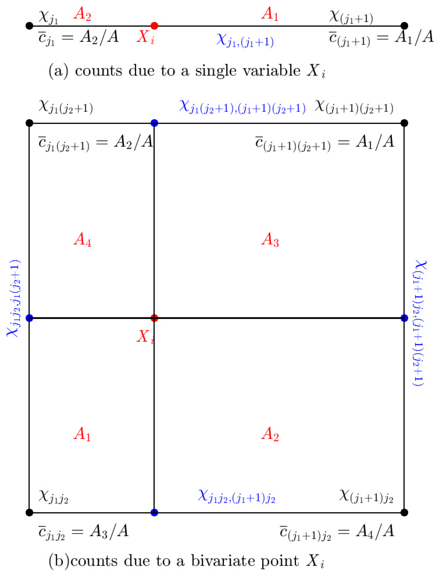
2.2.1. Computational Algorithm for Multivariate KDDE

Calculating $\nabla \overline{F}(x;H)$ on a given estimation grid $\chi$ by directly looping over the grid points and sample data points is time-consuming, especially for large n and/or $M$ values. To reduce the calculation burden, according to the algorithm of Wand [80], the KDDE can be a computationally efficient approximation by using a fast linear binning approximation [81,82]. Therefore, by supposing that $X_i$ falls into a hyper-rectangle (also called a bin) with 2^d facets and 2^d vertices, following Gramacki and Gramacki [77] and Wand [80], the calculation process of Equation (6) is detailed with three steps.

The first step is to convert the original sample data $X$ into grid counts using a fast linear binning approximation. Comparing the natural coordinate’s definition in Rao’s book [83] with the grid count’s definition in Chacón and Duong’s book [76], the grid count at a grid point of the hyper-rectangle due to $X_i$ is equal to the value of the natural coordinate at the same grid point. Then, these counts are accumulated into a large matrix C.

Take univariate data (d = 1) as an example, the hyper-rectangle (also called a bin) is a line segment with two endpoints ${\chi }_{j_1}$ and ${\chi }_{j_1+1}$. Then, suppose that the ith sample data $X_i$ is inside the line segment. Further, assume that the length of the bin is A and the length of the line segments, divided by $X_i$, are $A_1$ and $A_2$ as shown in Figure 1a. According to the natural coordinate’s definition, the grid counts correspond to the two endpoints ${\chi }_{j_1}$ and ${\chi }_{j_1+1}$ are expressed as ${\overline{c}}_{j_1}$ and ${\overline{c}}_{j_1+1}$, respectively. Then the counts are defined as

$${\overline{c}}_{j_1}=A_2/A, {\overline{c}}_{j_1+1}=A_1/A$$

(8)

To further illustrate the computational process of the multivariate KDDE in more detail, we focus on the bivariate case for the remainder of this section. Take a bivariable sample data (d = 2) as an example, the hyper-rectangle/bin is a rectangle, as shown in Figure 1b. Then, suppose that the ith sample data $X_i$ falls into a hyper-rectangle/bin whose vertices are ${\chi }_{j_1,j_2}$, ${\chi }_{j_1+1,j_2}$, ${\chi }_{j_1+1,j_2+1}$, and ${\chi }_{j_1,j_2+1}$. The areas of the rectangles subtended from $X_i$ are $A_1$, $A_2$, $A_3$, and $A_4$. The grid count is defined as the area of its diagonally opposite rectangle divided by the total area A of the bin. Thus,

$$\{\begin{array}{l}{\overline{c}}_{j_1,j_2}=A_3/A\hfill \\ {\overline{c}}_{\left(j_1+1\right),j_2}=A_4/A\hfill \\ {\overline{c}}_{j_1,\left(j_2+1\right)}=A_2/A\hfill \\ {\overline{c}}_{\left(j_1+1\right),\left(j_2+1\right)}=A_1/A\hfill \\ A_1+A_2+A_3+A_4=A\hfill \end{array}$$

(9)

By a similar process as above, extending it to the case of high-dimensional samples is easy. Then, the individual counts at the grid points are accumulated by looping this calculation over all sample data points. For a given estimation grid $\chi$ with a size of $M=M_1{M}_2$, the grid count $c_{l_1,l_2}$ at ${\chi }_{l_1,l_2}$ due to $X$ is given by

$$c_{l_1,l_2}={\displaystyle {\sum }_{i=1}^n{\overline{c}}_{l_1,l_2}\left(X_i\right)}$$

(10)

where, $l_k=1,\cdots ,M_k$, $1\le k\le d$, and the function ${\overline{c}}_{l_1,l_2}\left(X_i\right)$ is a natural coordinate value due $X_i$ on ${\chi }_{l_1,l_2}$.

Following Gramacki and Gramacki [77] and Wand [80], the fast linear binning approximation of Equation (6) at a grid point ${\chi }_{j_1,j_2}$ is the discrete convolution of grid counts and the kernel evaluations:

$$\nabla {\overline{F}}_{\mathrm{bin}}\left({\chi }_{j_1,j_2}\right)={\displaystyle \sum _{l_1=1}^{M_1}{\displaystyle \sum _{l_2=1}^{M_2}{c}_{l_1,l_2}\nabla K_H\left({\chi }_{j_1,j_2}-{\chi }_{l_1,l_2}\right)}}$$

(11)

The second step is to evaluate the kernel function on the same grid $\chi$. Equation (11) is rewritten in the bi-dimensional convolution form, as introduced by Wand [80]:

$$\nabla {\overline{F}}_{\mathrm{bin}}({\chi }_{j_1,j_2})={\displaystyle \sum _{l_1=-\left(M_1-1\right)}^{M_1-1}{\displaystyle \sum _{l_2=-\left(M_2-1\right)}^{M_2-1}{c}_{j_1-l_1,j_2-l_2}{k}_{l_1,l_2}}}$$

(12)

where $k_{l_1,l_2}=$$n^{-1}\nabla K_H\left(H_1{l}_{ 1},H_2{l}_{ 2}\right)$, and $c_{l_1,l_2}=0$, $\mathrm{for} \left(l_1,l_2\right)\notin$ $\{1,\dots ,M_1\}\times \{1,\dots ,M_2\}$.

The third step is to carry Equation (12) out by nested for-loops. However, its computational complexity is $O\left(M^2\right)$ time. Many fast algorithms of computing convolution were proposed, such as the Cook-Toom algorithm [84], the Agarwal-Cooley algorithm [85], and the Winograd algorithm [39], to reduce the computational complexity significantly.

In fact, KDE can also be considered a convolution [71,72]. The Winograd algorithm is known as a fast convolution to improve computational efficiency and save computational costs through the FFT [80]. This approach does not impose any restrictions on the kernel. The convolution between $c_{l_1,l_2}$ and $k_{l_1,l_2}$ can be carried out quickly by the FFT with only the operation $O\left(M{\displaystyle {\prod }_{j=1}^d\left(\log M_j\right)}\right)$. The convolution can be rewritten as [77,80,86]:

$$Y={\phi }^{-1}\left(\phi \left(C\right)\phi \left(K\right)\right)$$

(13)

where $\phi$ is the discrete Fourier transform and ${\phi }^{-1}$ is its inverse transform. Letting $P_k$ be a power of 2 greater than size $M_k$, and $Y$ be a $P_1\times P_2$ matrix. Writing $0_{m;n}$ for the $\left(m\times n\right)$ zero matrix. The zero-padded version of the binning counts $C$ is

$$C=\left[\begin{array}{ccccc}{0}_{M_1-1;M_2-1}& & 0_{M_1-1;M_2}& & 0_{M_1-1;P_2-2M_2+1}\\ & c_{1,1}& \cdots & c_{1,M_2}& \\ 0_{M_1;M_2-1}& ⋮& & ⋮& 0_{M_1;P_2-2M_2+1}\\ & c_{M_1,1}& \cdots & c_{M_1,M_2}& \\ 0_{P_1-2M_1+1;M_2-1}& & 0_{P_1-2M_1+1;M_2}& & 0_{P_1-2M_1+1;P_2-2M_2+1}\end{array}\right]$$

(14)

and of the kernel evaluations $K$ is

$$K=\left[\begin{array}{cc}\begin{array}{ccccc}{k}_{-M_1,-M_2}& \cdots & k_{-M_1,0}& \cdots & k_{-M_1,M_2}\\ ⋮& & ⋮& & ⋮\\ k_{0,-M_2}& \cdots & k_{0,0}& \cdots & k_{0,M_2}\\ ⋮& & ⋮& & ⋮\\ k_{M_1,-M_2}& \cdots & k_{M_1,0}& \cdots & k_{M_1,M_2}\end{array}\hfill & \begin{array}{c}\\ \\ 0_{2M_1+1;P_2-2M_2+1}\\ \\ \end{array}\hfill \\ \begin{array}{ccccc}& & & 0_{P_1-2M_1+1;P_2-2M_2+1}& \end{array}\hfill & 0_{P_1-2M_1+1;P_2-2M_2+1}\hfill \end{array}\right]$$

(15)

Details about zero-padding versions of involved matrices for performing the FFT operation can be found instance in Teukolsky et al. (1992, Chapter 13) [87] and Arndt (2010, Chapter 22) [88].

The result of the approximate density estimator from Equation (12) evaluated on the estimation grid $\chi$ is

$$\nabla {\overline{F}}_{\mathrm{bin}}\left(·;H\right)={\left({\displaystyle {\prod }_{j=1}^d{P}_j}\right)}^{-1}real\left(Y\left[\left(2M_1-1\right):\left(3M_1-2\right),\left(2M_2-1\right):\left(3M_2-2\right)\right]\right)$$

(16)

where the function $real(\cdot )$ returns the real part of the complex number, and $Y\left[ro{w}_1:ro{w}_2,co{l}_1:co{l}_2\right]$ denotes the submatrix of $Y$ formed by selecting the elements in rows $ro{w}_1$ to $ro{w}_2$ and columns $co{l}_1$ to $co{l}_2$. For simplicity, Equations (14) and (15) only present two-dimensional variants, which are easily extended to the higher-dimensional case. The result of Equation (16) is a probability or probability value, written as the p-value. This procedure is given in Algorithm 1.

In line 1, the gridded data $g_{\alpha },g_{\alpha \beta }\left(\alpha ,\beta \in \left(x,y,z\right)\right)$ are obtained by survey, forward modeling, or derived from field data using FFT.

In lines 2–4, we select a moving window with size $w_x\times w_y$ to traverse the gridded data using Equation (4) to yield a Euler solution dataset associated with causative sources. We found that simply using a fixed-size moving window for different-sized geological targets would lose the ability to distinguish spurious solutions. Therefore, we use a fixed-size moving window for synthetic models and a series of moving windows with a size ranging from 4 × 4 to 12 × 12 to traverse the field data throughout this paper.

In lines 5–9, we set the problem dimensionality d, choose a variant of the Euler solution dataset as a data instance, and calculate its marginal sample’s minima a and maxima b. Due to grid size being inversely proportional to bandwidth, based on Equation (7), we select the size M₁ × … × M_d or take H as an input parameter, then construct an estimation grid to cover exactly [a₁, b₁] × … × [a_d, b_d] for the input sample data.

In lines 10–17, grid counts $c$ are obtained by binning the sample data into an estimation grid with the fast linear binning approximation in lines 10–13, and kernel function evaluations $k$ are calculated based on Equation (13) in lines 14–16. Then, the zero-padded versions of the grid count $C$ and the kernel evaluation $K$ are constructed for carrying out $Y={\phi }^{-1}\left(\phi \left(C\right)\phi \left(K\right)\right)$ with the FFT operations. In the end, the probability density distributions $\nabla {\overline{F}}_{\mathrm{bin}}$ are obtained by multivariate KDDE to discriminate spurious solutions and isolate complex geological sources. All the tests were carried out on a server equipped with an Intel(R) Xeon(R) Gold 5117 CPU and 64 GB of memory.

Algorithm 1. Multivariate kernel density derivative estimation (KDDE).

$\mathrm{input}:g_z,w_x,w_y,M or H$

$\begin{array}{l}\begin{array}{l}1:\mathrm{Calculate} g_{\alpha },g_{\alpha \beta }\left(\alpha ,\beta \in \left(x,y,z\right)\right)\\ 2:\mathrm{for} i\mathrm{-th} \mathrm{moving} \mathrm{window}\\ 3:\hspace{1em}\hspace{1em}\mathrm{Solve} \mathrm{Equation} \left(6\right) \mathrm{to} \mathrm{obtain} m_i={\left[x_o^i,y_o^i,z_o^i,N_{}^i\right]}^{\mathrm{T}}\\ 4:\mathrm{endfor}\\ 5:\mathrm{Set} \mathrm{the} \mathrm{problem} \mathrm{dimensionality} d\\ 6:\mathrm{Pick} \mathrm{a} \mathrm{variant} \mathrm{of} \mathrm{Euler} \mathrm{solutions} \mathrm{as} \left\{X_1,\dots ,X_n\right\}\\ 7:\mathrm{Calculate} a,b \\ 8: \mathrm{Calculate} H \mathrm{by} \mathrm{predefined} M, \mathrm{vice} \mathrm{versa} \\ 9:\mathrm{Binning} \mathrm{grid} \mathrm{to} \mathrm{cover}\left[a_1,b_1\right]\times \cdots \times \left[a_d,b_d\right]\\ 10:\mathrm{Initialise} P_k:=2^{\lceil {\log }_2\left(2M_k\right)\rceil },1\le k\le d\\ 11:\mathrm{for} l_1,\cdots ,l_d :=1 \mathrm{to} M_1,\cdots ,M_d\\ 12:\hspace{1em}\hspace{1em} \mathrm{Compute} \mathrm{binning} \mathrm{counts} c_{l_1,\cdots ,l_d}\\ 13:\mathrm{endfor}\\ 14:\mathrm{for} l_1,\cdots ,l_d :=-M_1,\cdots ,-M_d \mathrm{to} M_1,\cdots ,M_d \\ 15:\hspace{1em}\hspace{1em}\mathrm{Evaluate} \mathrm{kernel} \mathrm{functions} k_{l_1,\cdots ,l_d}\\ 16:\mathrm{endfor}\\ 17:\mathrm{Create} \mathrm{zero}-\mathrm{padded} \mathrm{versions} \mathrm{of} \mathrm{counts} C \mathrm{and} \mathrm{of} \mathrm{kernel} \mathrm{matrices} K \\ 18:\mathrm{Carry} \mathrm{out} \mathrm{the} \mathrm{FFT} \mathrm{operations} Y={\phi }^{-1}\left(\phi \left(C\right)\phi \left(K\right)\right)\\ 19:\mathrm{Use} \mathrm{Equation} \left(17\right) \mathrm{to} \mathrm{extract} \mathrm{the} \mathrm{result} \mathrm{of} \mathrm{KDDE}\end{array}\hfill \end{array}$

$\mathrm{output}:\nabla \stackrel{\wedge }{F_{\mathrm{bin}}}\left(·;H\right)$

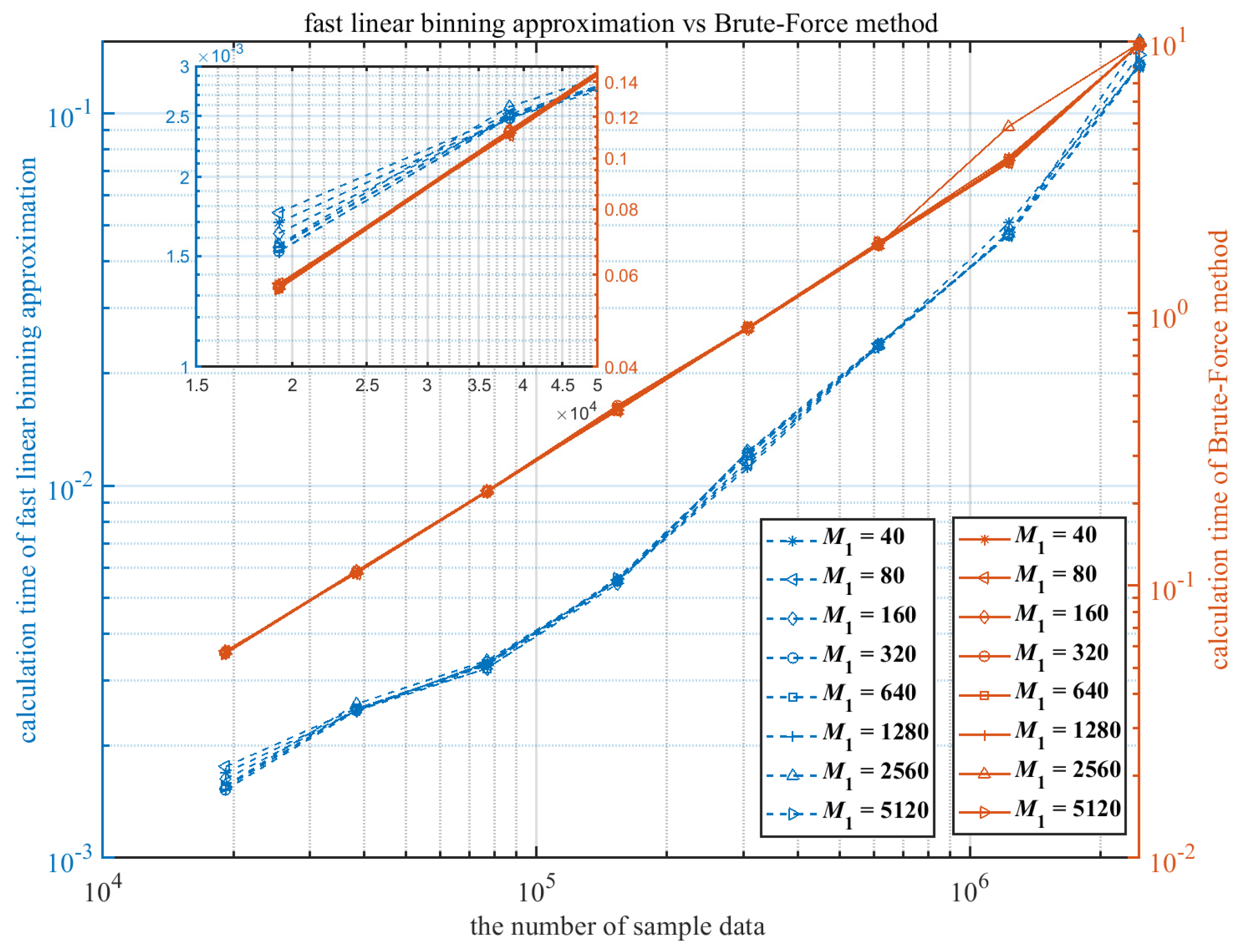
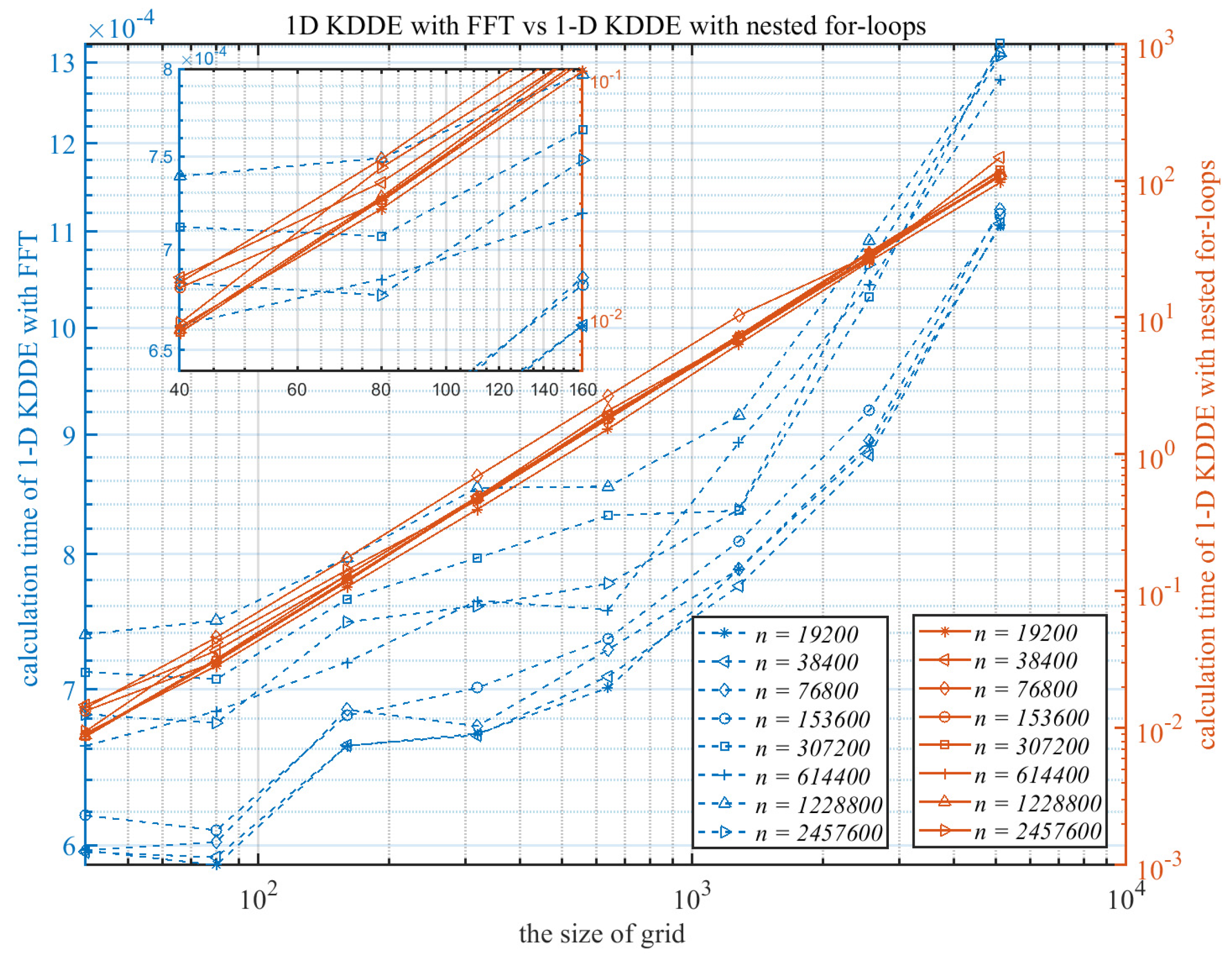
2.2.2. Computational Performance of Multivariate KDDE

To verify the computational efficiency of the fast linear binning approximation and multivariate KDDE proposed in this paper, we used the following parameters: $\mu$ = {−2, 0, 2} and $\delta$ = {1/6, 1/2, 1/3}, to construct eight data instances, which are drawn from a function $f(\mu ,\delta ,n)={\displaystyle {\sum }_{i=1}^3{\mu }_i+{\delta }_i\times randn(n,1)}$, with n = 19,200, 38,400, 76,800, 153,600, 307,200, 614,400, 1,228,800, and 2,457,600, respectively. Here, $randn(·,1)$ is 1-D normally distributed random numbers function. For the convenience of comparative analysis, the performance for calculating grid counts of the Brute-Force algorithm and the fast linear binning approximation is carried out by looping eight data instances over a series of one-dimensional grids with different-sized M₁ = 40, 80, 160, 320, 640, 1280, 2560, and 5120, respectively.

Two relatively tight line clusters are formed in Figure 2, indicating that using different-sized grids in fast linear binning approximation and the Brute–Force method does not significantly impact the computation time. In general, as the number of sample data increases, such as in the partially enlarged drawing, the corresponding computation time increases linearly. Meanwhile, the computation time of both algorithms tends to increase sharply with the increase in the number of observation samples. Compared with the Brute-Force calculation, the fast linear binning approximation can significantly save computational times by about an order of magnitude. However, the accelerating tendency of this algorithm gradually weakens with the number of observation samples increasing, which may be affected by the computer performance.

Based on the above eight data instances, we verify the computational performance of the multivariate KDDE. The 1-D KDDE was calculated using nested for-loops and FFT based on Equation (16) over a series of grids = [40, 80, 160, 320, 640, 1280, 2560, 5120], respectively.

In Figure 3, the computation time of both algorithms increases slightly as the number of observation samples increases. However, the result of 1-D KDDE with nested for-loops is more pronounced, for example, when the grid size is not greater than 160 in the partially enlarged drawing. Along with the increase in grid size, the 1-D KDDE with FFT is more computationally efficient by about 3–4 orders of magnitude than the 1-D KDDE with nested for-loops. However, as the grid size increases (i.e., M₁ > 1280), the accelerating tendency of 1-D KDDE with FFT gradually decreases, perhaps owing to computer performance. Fortunately, we do not adopt such a large estimation grid in practical applications.

3. Results

3.1. Model Studies

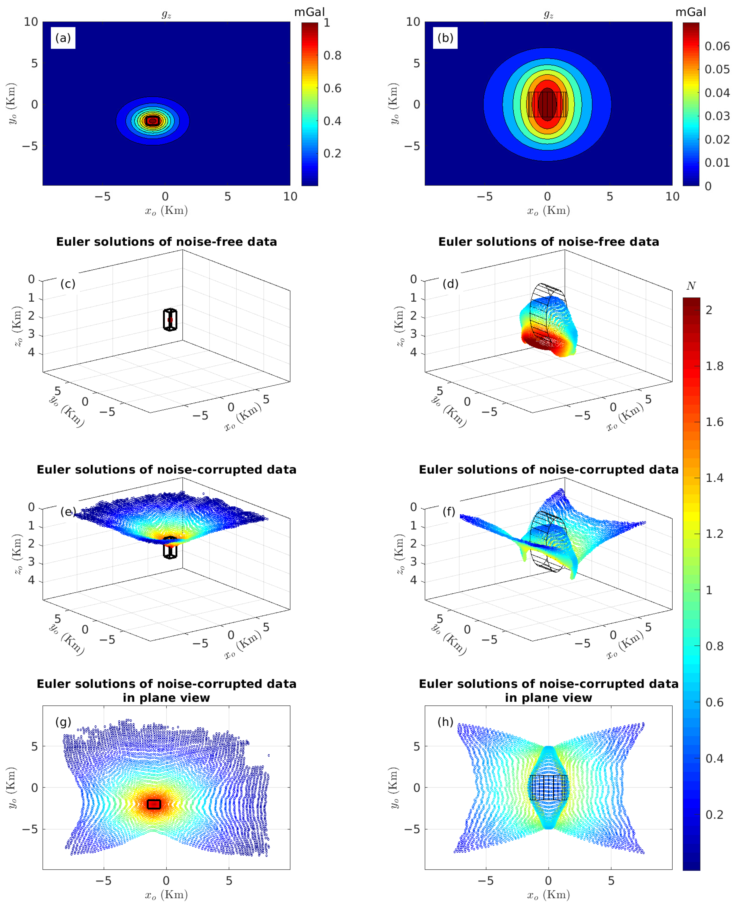
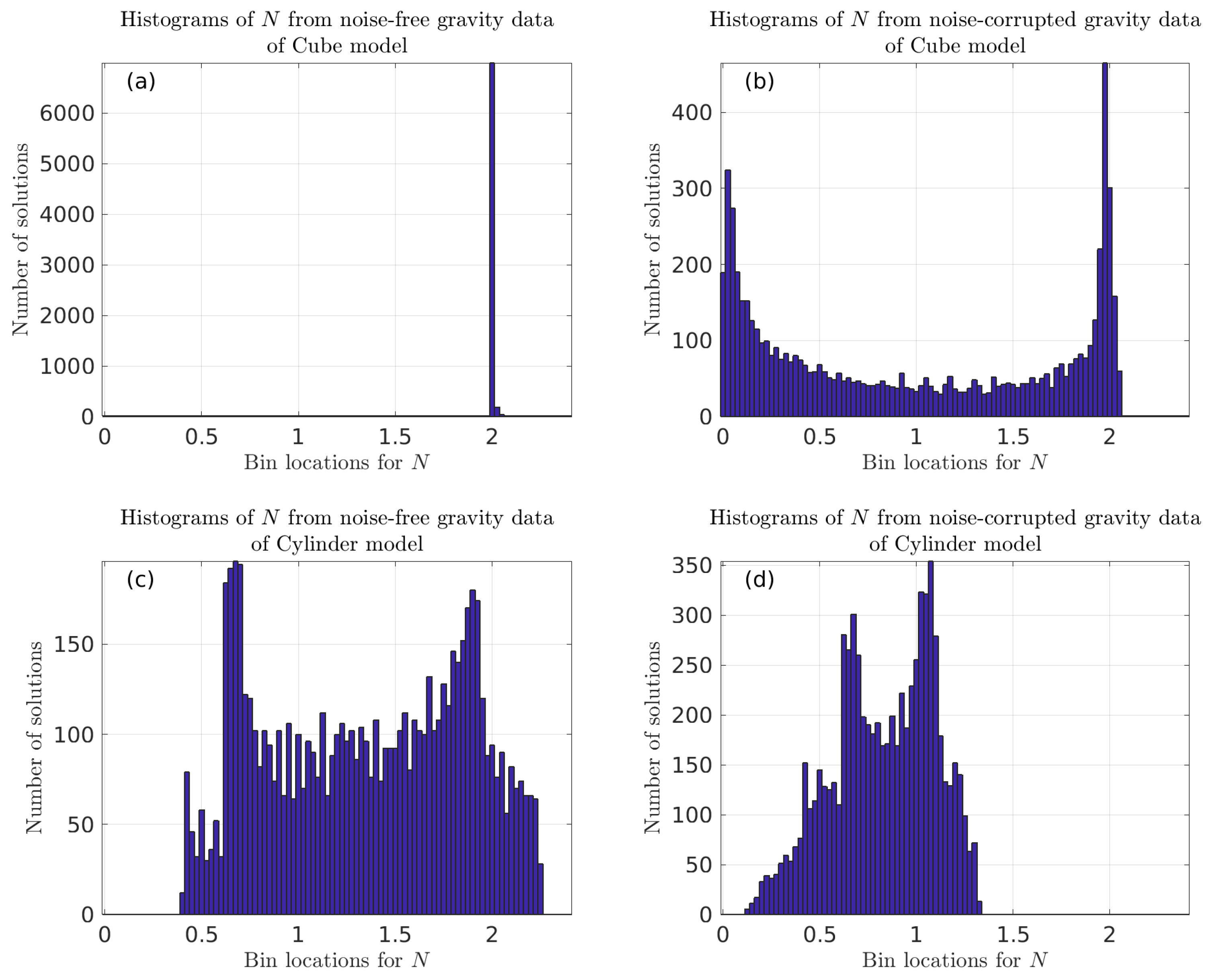
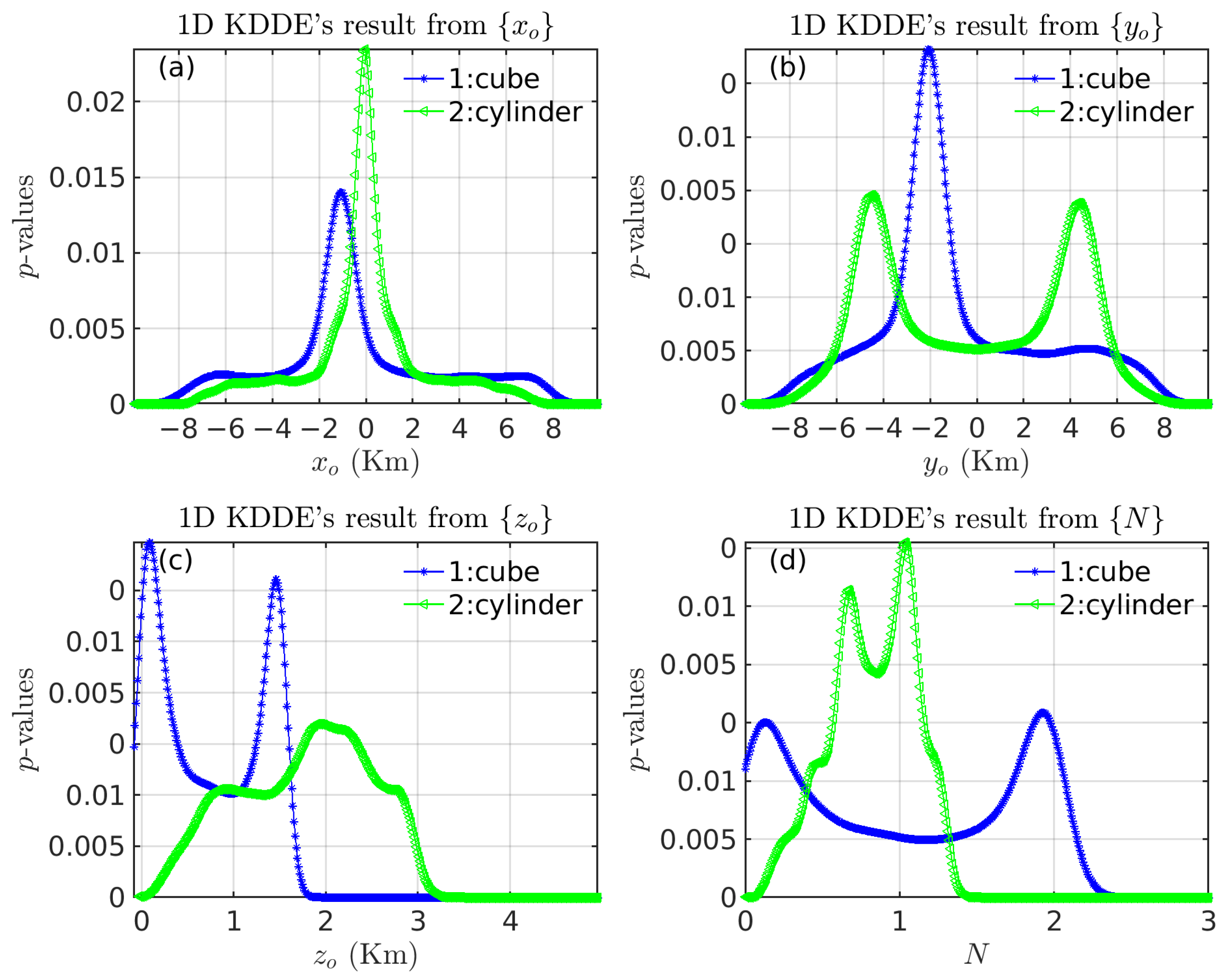
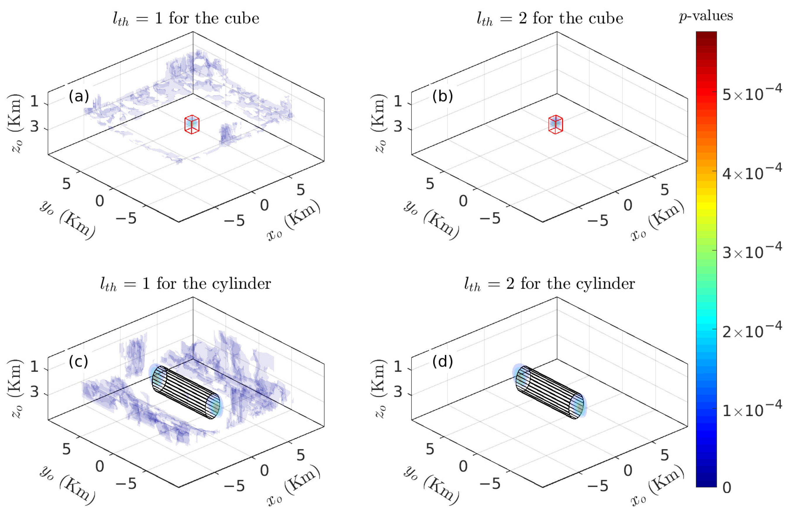
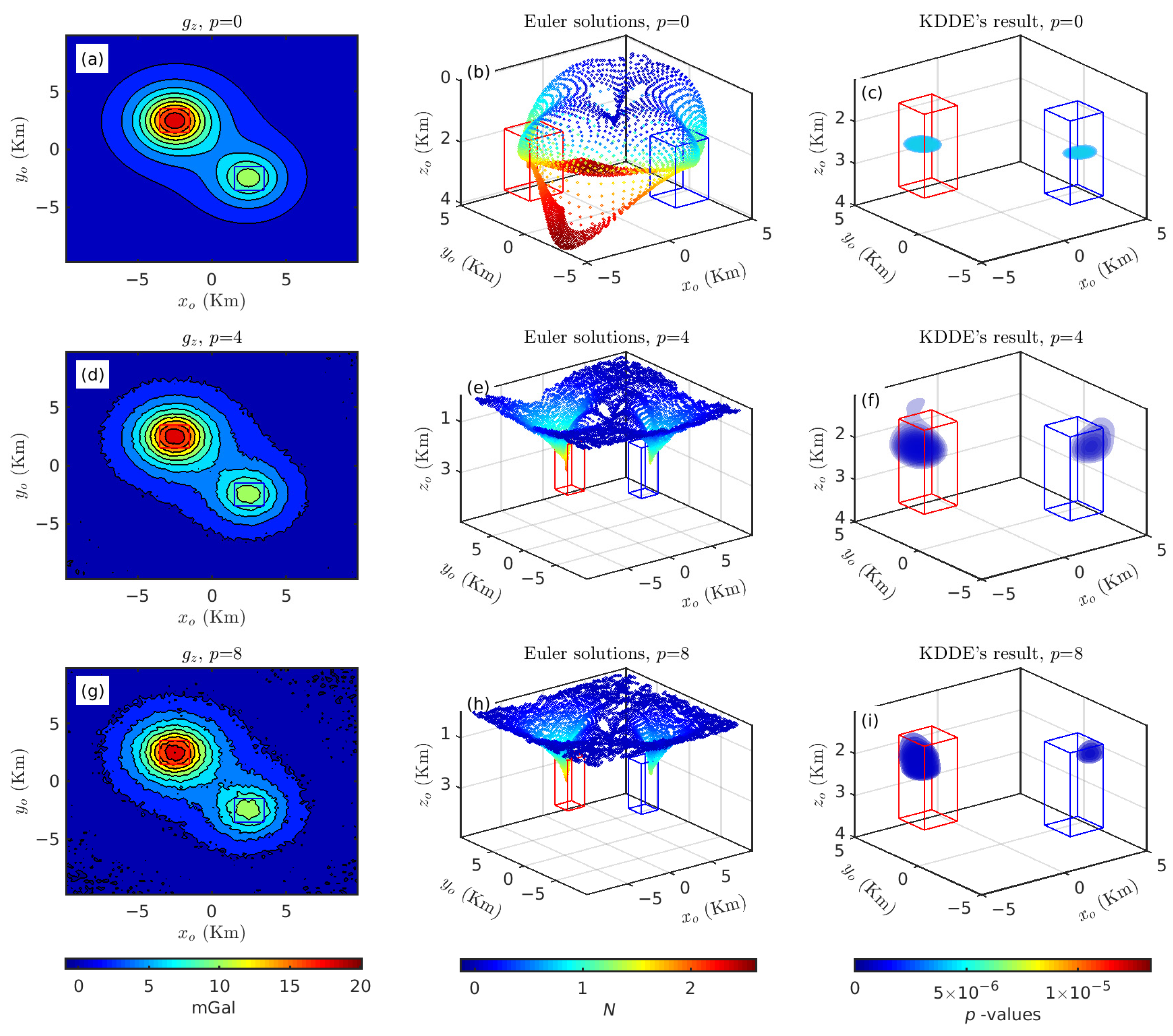
3.1.1. Verification of the Validity of the Multivariate KDDE Algorithm

Two simple models (cube and cylinder) were established to validate the tensor Euler deconvolution algorithm and the multivariate KDDE algorithm. Both models have a density contrast of 0.36 g/cm³. The geometric parameters and theoretical N of the two models are shown in

Table 1. The geometric parameters and structural indices for two simple models.

Model	Centroid	Radii	Lengths	Theoretical N
Cube	(−1000, −2000, 1500)	/	1000 × 1000 × 1000	2
Cylinder	(0, 0, 2500)	1000	4000	1~2

. Then, a rectangular survey grid, with 200 points, with 100 m grid interval in both horizontal directions, was employed for forward processing. The study used the noise-free FTG data obtained by the analytical solutions and noise-corrupted data, which contaminated the FTG data by Gaussian noise with zero-mean and variance $\sigma \left(p\right)$, which is a function of the percentage $p$ of input data:

$$\sigma \left(p\right)=\frac{p}{100}\sqrt{\frac{{\displaystyle {\sum }_{i=1}^{n_{obs}}ob{s}_i^2}}{n_{obs}}}$$

(17)

where $ob{s}_i$ is the ith data and $n_{obs}$ is the number of the given data sample.

Equations (1)–(3) were applied to the noise-free and the noise-corrupted FTG data to estimate x_o, y_o, z_o, and N. The size of the square moving window was $w_x=w_y=15$. As shown in Figure 4, the solutions were filtered by N > 0.

As Figure 4b shows, the Euler solutions were around the center of the cylinder and their SIs (N ≈ 2) were consistent with the theoretical values. In Figure 4c,d, the SIs of the Euler solutions in red were consistent with their theoretical values (Table 1). Compared to the cylinder’s Euler solutions, the cube’s ones formed a tighter cluster in Figure 4c. There were no spurious solutions in the Euler solution dataset in Figure 4c,d. Figure 4e–h show that the magnitudes of the SIs for the Euler solutions around the anomalous sources were consistent with their theoretical values. However, there were many more spurious solutions.

The histogram was used to discriminate spurious Euler solutions [34]. When there was no noise in the input data, the tensor Euler deconvolution yielded very pure solutions, indicating that many similar or duplicate solutions were generated and may be clustered tightly in the vicinity of the real sources (Figure 4c and Figure 5a). Conversely, the tensor Euler deconvolution produced many spurious solutions in Figure 4e–h and Figure 5b,d. This phenomenon shows that the tensor Euler deconvolution was susceptible to noise. Moreover, as for the cylinder model, the SIs derived from the noiseless data fluctuated between 0.41 and 2.25; in contrast, the solutions derived from noise-corrupted data tended to diverge because their maximum N value was smaller than the former.

For comparison, using the 7th, 8th, and 9th strategies proposed by FitzGerald et al. [34] to select the most reliable Euler solutions, we could effectively remove spurious solutions (such as N > 3 or N < 0) to quickly determine the anomaly source’s location in Figure 5c,d. Compared to the Euler solutions drawn from the noise-free data, the magnitudes of all SIs decreased for the ones derived from the noise-corrupted data in the cylinder model. Ravat [22] pointed out that the N changes discontinuously as the source-to-observation distance changes. Therefore, only using the SIs made it difficult to determine optimal solutions.

To overcome those difficulties, we used multivariate KDDE to estimate the combinations of Euler solutions. Peaks could be obtained for each probability density curve using the findpeaks function. In Figure 6a, the coordinates x of the two peaks were −1.0 km and 0 km, respectively, consistent with their theoretical values. This correspondence also appeared in Figure 6b. In contrast, in Figure 6c,d, the leftmost peak of each curve corresponded to shallow-buried Euler solutions, considered spurious ones; the rightmost peak of each curve corresponded to their theoretical values.

Generally, a simple geological body has only one peak. However, a complex geological body has two or more peaks. For example, in Figure 6b–d, there were two peaks for each curve, leading to difficulty in selecting the optimal Euler solutions. This phenomenon resulted in the histograms and probability density curves being unable to intuitively characterize the underground space, as shown in Figure 5 and Figure 6.

The locations and SIs were easily interpreted in this study using the 2-D KDDE. However, there were too many 2-D combinations of Euler solutions, so interpreting simultaneously all probability density images was difficult. Furthermore, visualization of the 5-D results {x_o, y_o, z_o, N, p-value}, obtained by multivariate KDDE to estimate the entire Euler solution dataset, was very challenging. The results derived from the three subsets {x_o, y_o, N}, {x_o, z_o, N}, and {y_o, z_o, N} need to be more intuitive and straightforward. The interpretation of the Euler solution datasets using 3-D KDDE relied mainly on the subset {x_o, y_o, z_o}, with assistance from other subsets. Therefore, we illustrated only results of the subset {x_o, y_o, z_o} in the remainder of this paper.

Then, we obtained four isosurface subplots of the probability density distributions using 3D-KDDE for the two models in Figure 7. The isosurfaces throughout this paper had 20 levels whose p-values were evenly spaced points between the minimum and maximum values of probability density distribution. The isosurface levels from the l_th to the last were plotted. The twenty isosurface levels (lth = 1) were plotted in Figure 7a,c, and many small contours corresponded to the spurious solutions. Conversely, when l_th = 2, these contours were removed in Figure 7b,d. Therefore, we could determine the l_th to locate meaningful geological bodies.

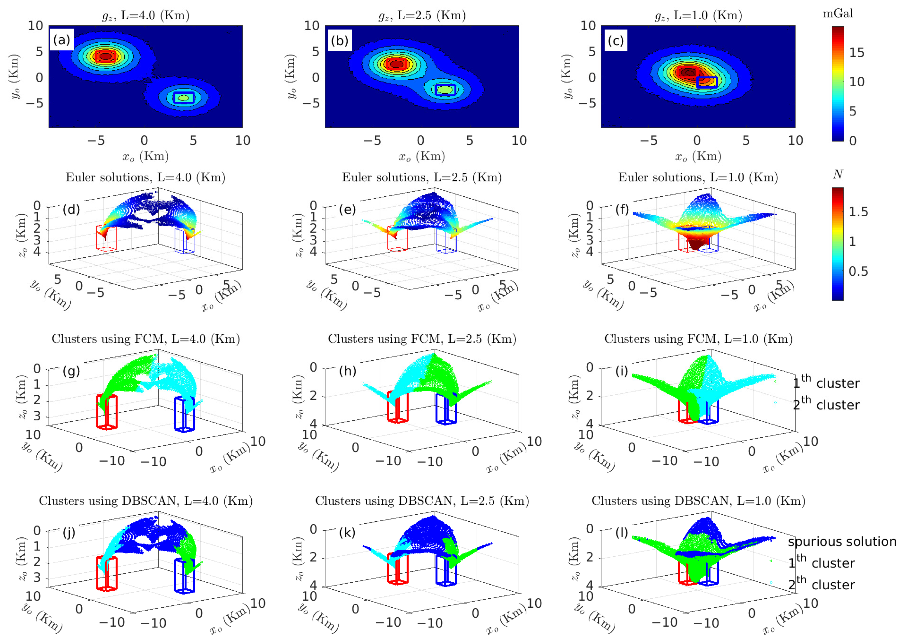
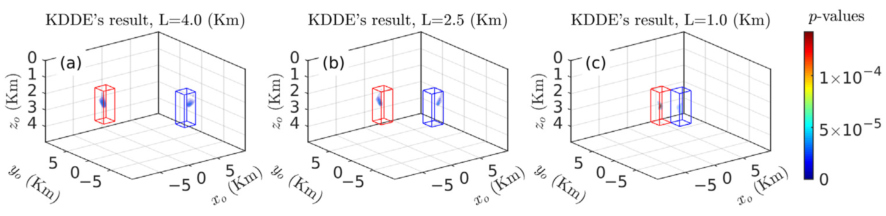
3.1.2. Sensitivity of 3-D KDDE to Separations

To assess the performance of the proposed algorithm in distinguishing adjacent anomaly sources, we used two similar causative sources with separations of L = 4.0 km, 2.5 km, and 1.0 km to form three models. These separations of L allowed two causative bodies to simultaneously approach each other in the x- and y- directions. The parameters of the two causative bodies were listed in

Table 2. The geometric parameters for the three synthetic models with various separations.

Separations	Centroid of Left Cube	Centroid of Right Cube
4000	(−4000, 4000, 2500)	(4000, −4000, 2500)
2500	(−2500, 2500, 2500)	(2500, −2500, 2500)
1000	(−1000, 1000, 2500)	(1000, −1000, 2500)

. The rectangular survey grid was divided into 40,000 = 200 × 200 observation points with an interval of 100 m. The 3-D KDDE was used in the current investigation to analyze the subset {x_o, y_o, z_o} derived from the FTG data contaminated by 3% Gaussian noise based on Equation (17).

As the separation L decreased, it became more difficult to distinguish the two adjacent cubes using the Euler solutions in Figure 8d–f. Furthermore, in Figure 8g–i, the FCM algorithm, whose performance depended on the preset number of clusters, effectively distinguished adjacent anomaly sources, and did not eliminate spurious solutions. In contrast, when the distance between adjacent anomaly sources was considerable, the density-based spatial clustering of applications with noise (DBSCAN) could determine some spurious solutions, such as the Euler solutions in green in Figure 8j,k. Nevertheless, if the two anomaly sources were close (Figure 8l), this method could not effectively separate them or discriminate spurious solutions.

In addition, FitzGerald et al. [34] reported that Euler deconvolution yields many similar or duplicate solutions, which may tightly cluster in the vicinity of real sources. Therefore, the density cluster is essential for classifying Euler solutions [65,89]. This main feature could discriminate spurious solutions to indicate adjacent anomalous sources. Therefore, we used the multivariate KDDE, which has the advantages of asymptotic unbiasedness, square consistency, and uniform convergence [75,76], to overcome this difficulty.

Figure 9 illustrates the partitioning of geological bodies using the 3-D KDDE to estimate the subset {x_o, y_o, z_o}. Compared to other techniques for separating adjacent anomalous sources, as shown in Figure 8, two probability density peaks directly discriminated the two geological bodies with varied separations.

3.1.3. Sensitivity of 3-D KDDE to Gaussian Noises

If the signal-to-noise ratio of the input data is low, the corresponding solution will be masked, which makes it challenging to outline the boundaries of geological targets. Various criteria for clustering methods have been introduced to reject spurious solutions with low tolerance [9,34,38]. However, clustering methods could not discriminate spurious solutions efficiently in shallow sources and neighboring bodies [50,51]. For this reason, to study the sensitivity of our methods to Gaussian noise, 3-D KDDE was applied to the subset {x_o, y_o, z_o} obtained by tensor Euler deconvolution derived from a synthetic model containing two cubes with a separation L of 2.5 km (Figure 9b). In Figure 10, as the noise percentage grows, there were increasingly disturbed contours in the gravity maps, and the number of Euler solutions with low SIs dramatically increased. Conversely, because spurious solutions were more unstable and their numbers increased, their corresponding probability density contours had tiny values and were removed by lth = 1. Therefore, the value of probability density isosurfaces increased after normalization. The estimated locations derived from 4-D probability density distributions were very close to the theoretical locations of the synthetic models, despite the noise percentage being equal to 8% ($p=8$). Although the tensor Euler deconvolution method is susceptible to noise [90], it was concluded that the 3-D KDDE results were reliable.

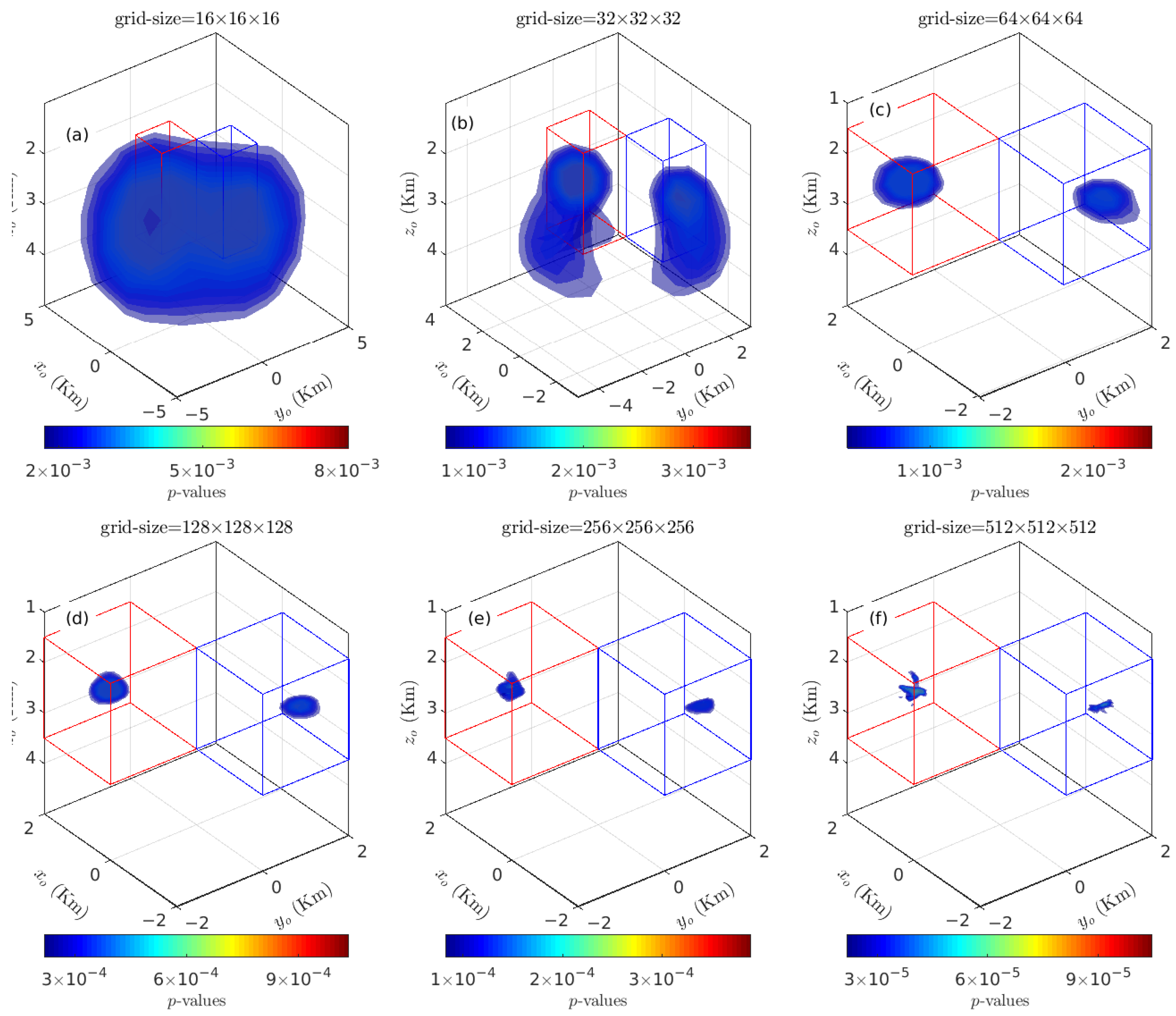
3.1.4. Sensitivity of 3-D KDDE to Grid Size

The estimated effect in multivariate KDDE mainly depends on the bandwidth or grid size. For a given data sample, its marginal sample maximum and minimum values are constant, and its grid size is inversely proportional to its bandwidth. The 3-D KDDE, in conjunction with the subset {x_o, y_o, z_o}, was carried out with different-sized cubic grids, whose length along one direction was 16, 32, 64, 128, 256, and 512, to analyze its sensitivity to grid size and its computational time was 0.0113, 0.0251, 0.1017, 0.7271, 7.8461, and 51.7940 s, respectively.

As tensor Euler deconvolution produces many similar or duplicate solutions, these solutions may cluster closely together in the vicinity of the true sources [34]. Figure 11 shows that as the grid size/bandwidth increased/decreased, the probability density distribution formed a tiny cluster, which was not conducive to determining the spatial distribution of anomalous sources but could effectively determine the centroid of the density structure. Because we constructed an efficient multivariate KDDE algorithm (in Algorithm 1), it was possible to isolate complex geological targets by trying different-sized girds.

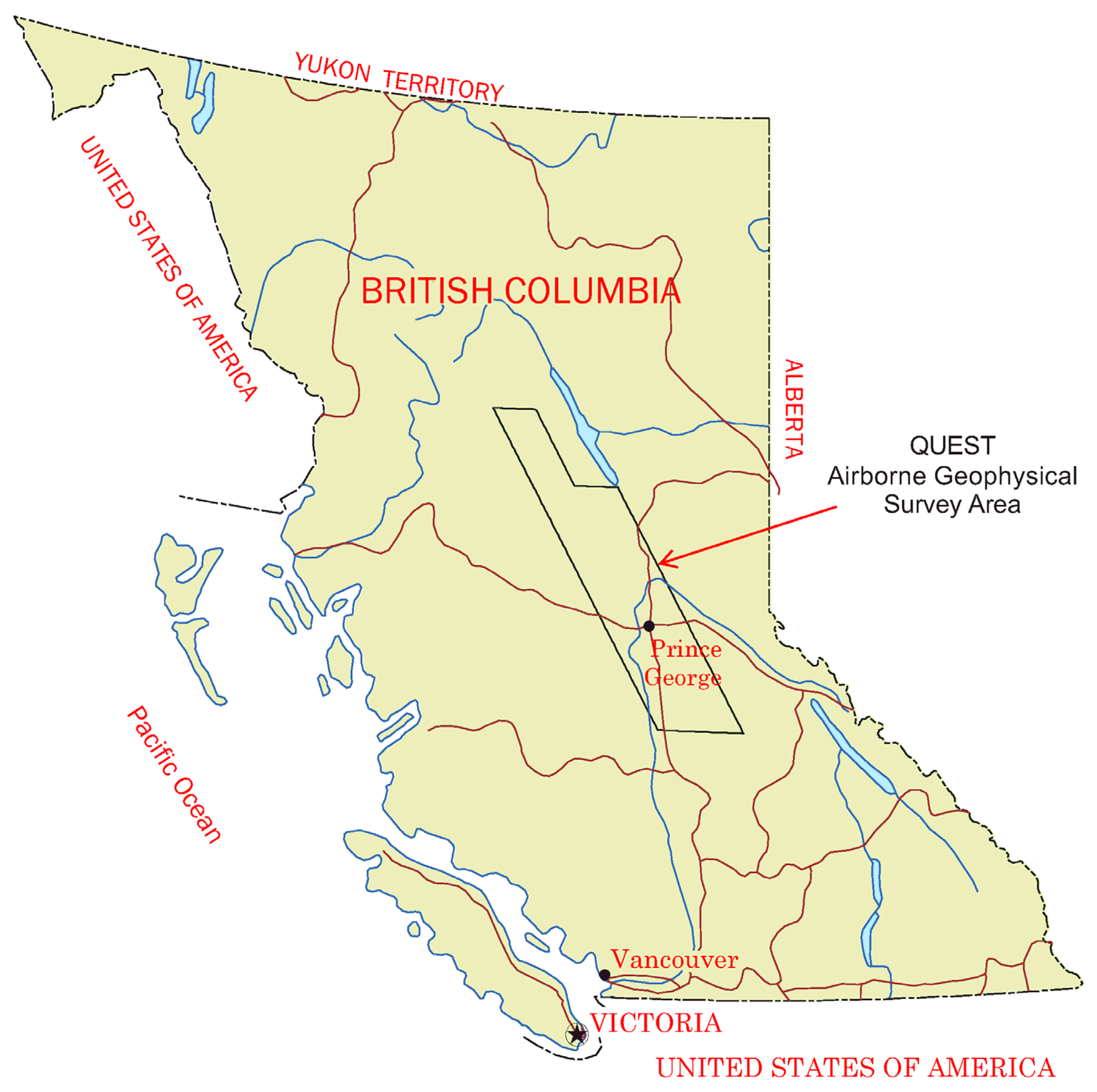
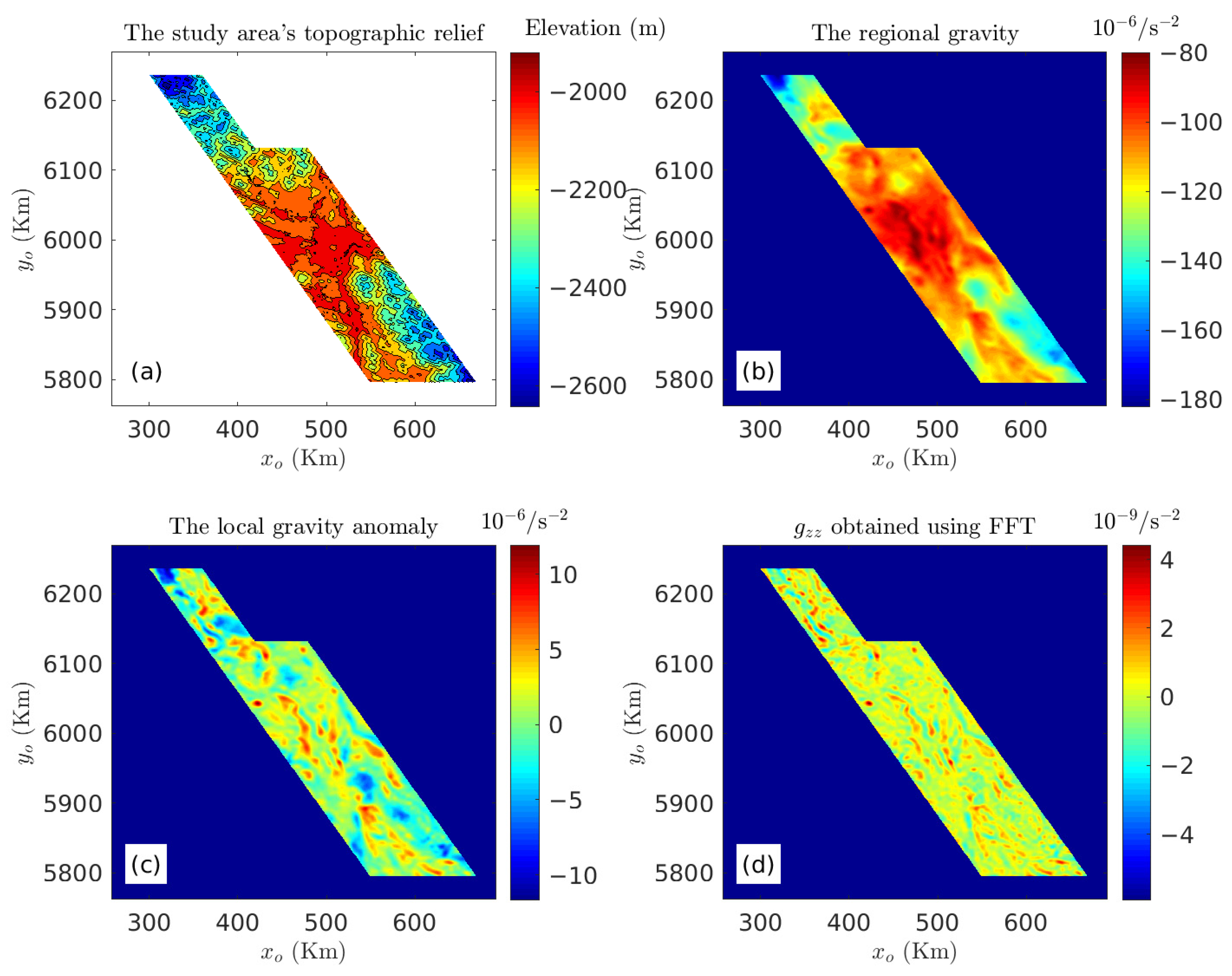
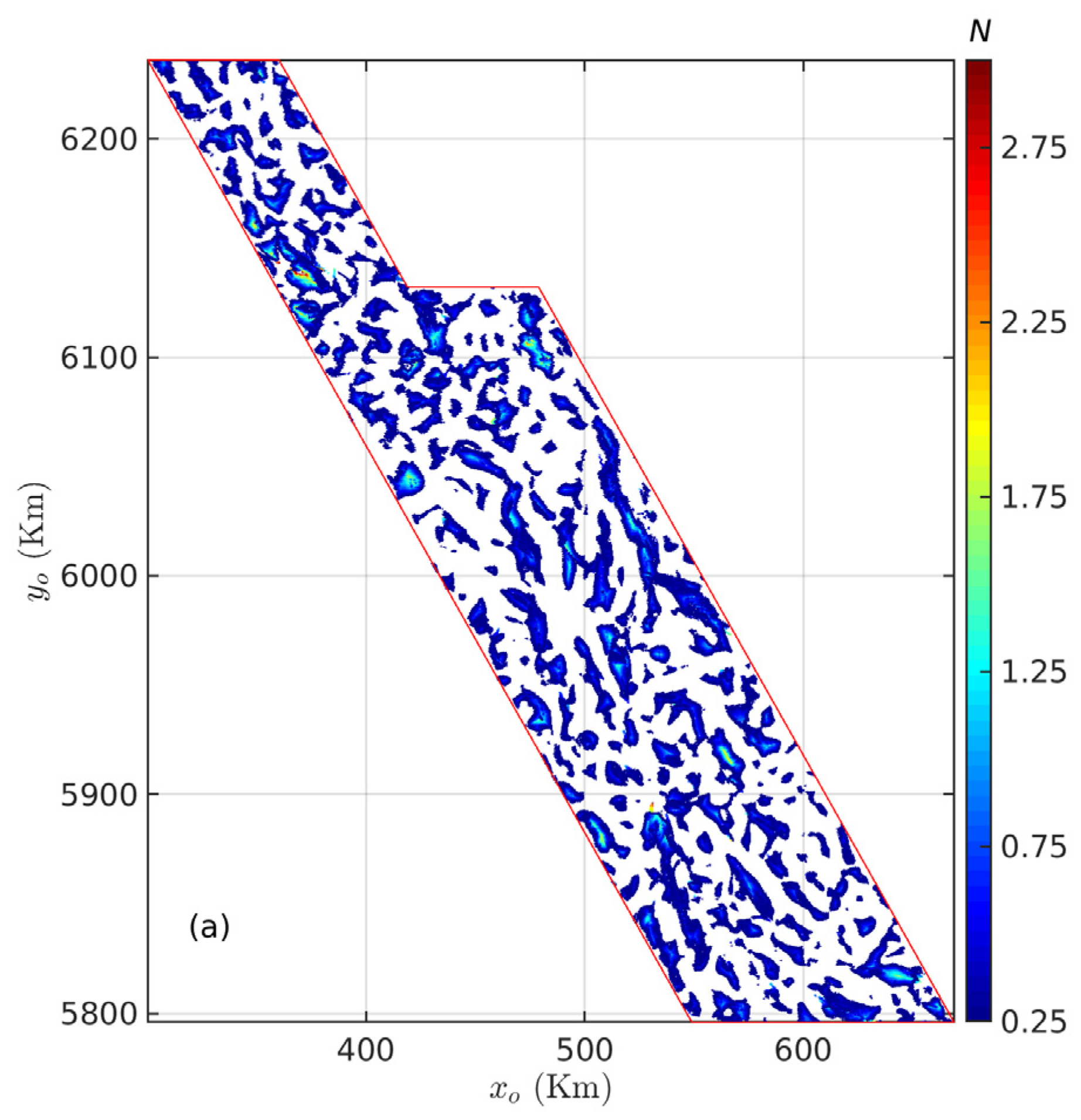
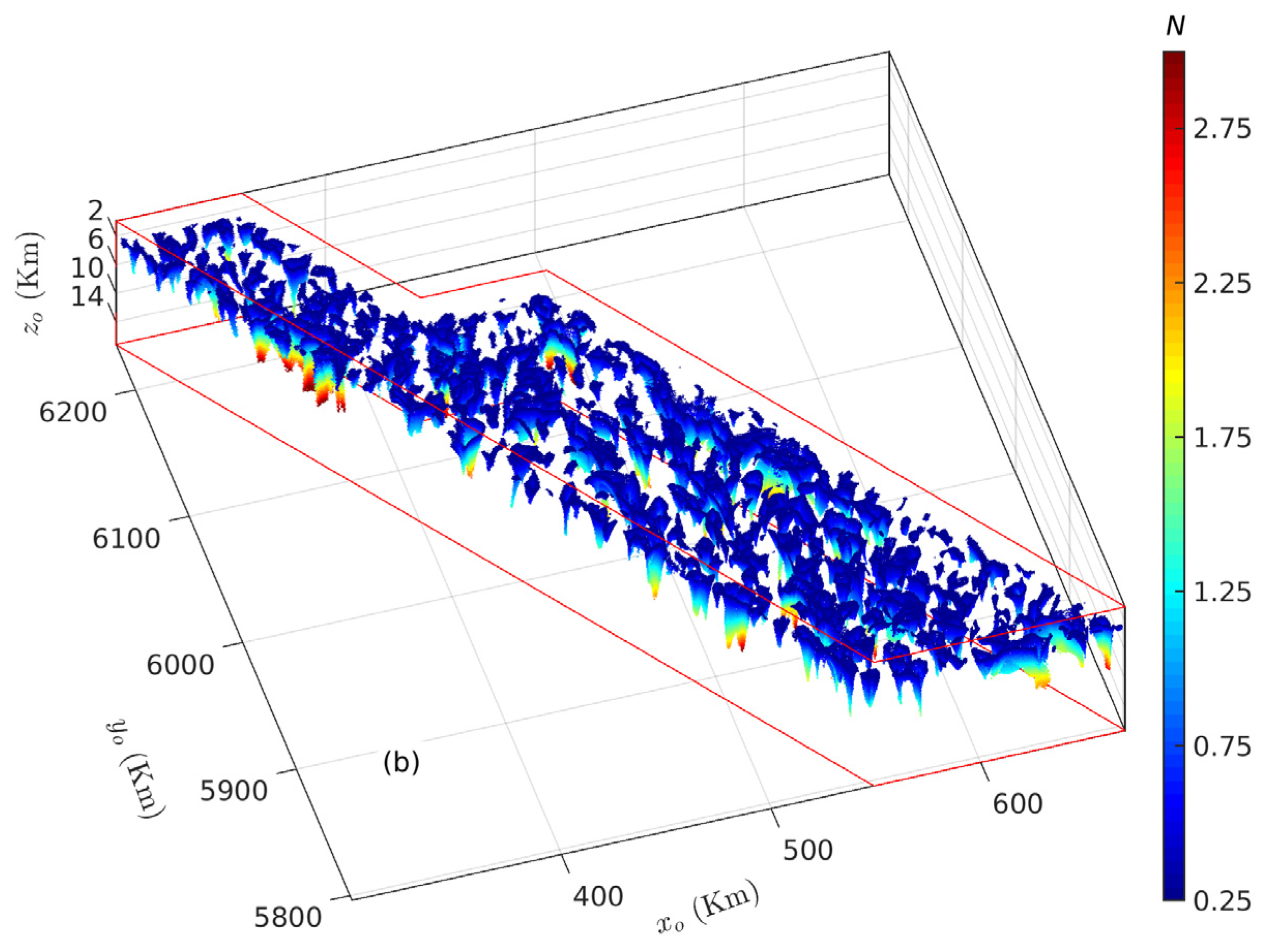
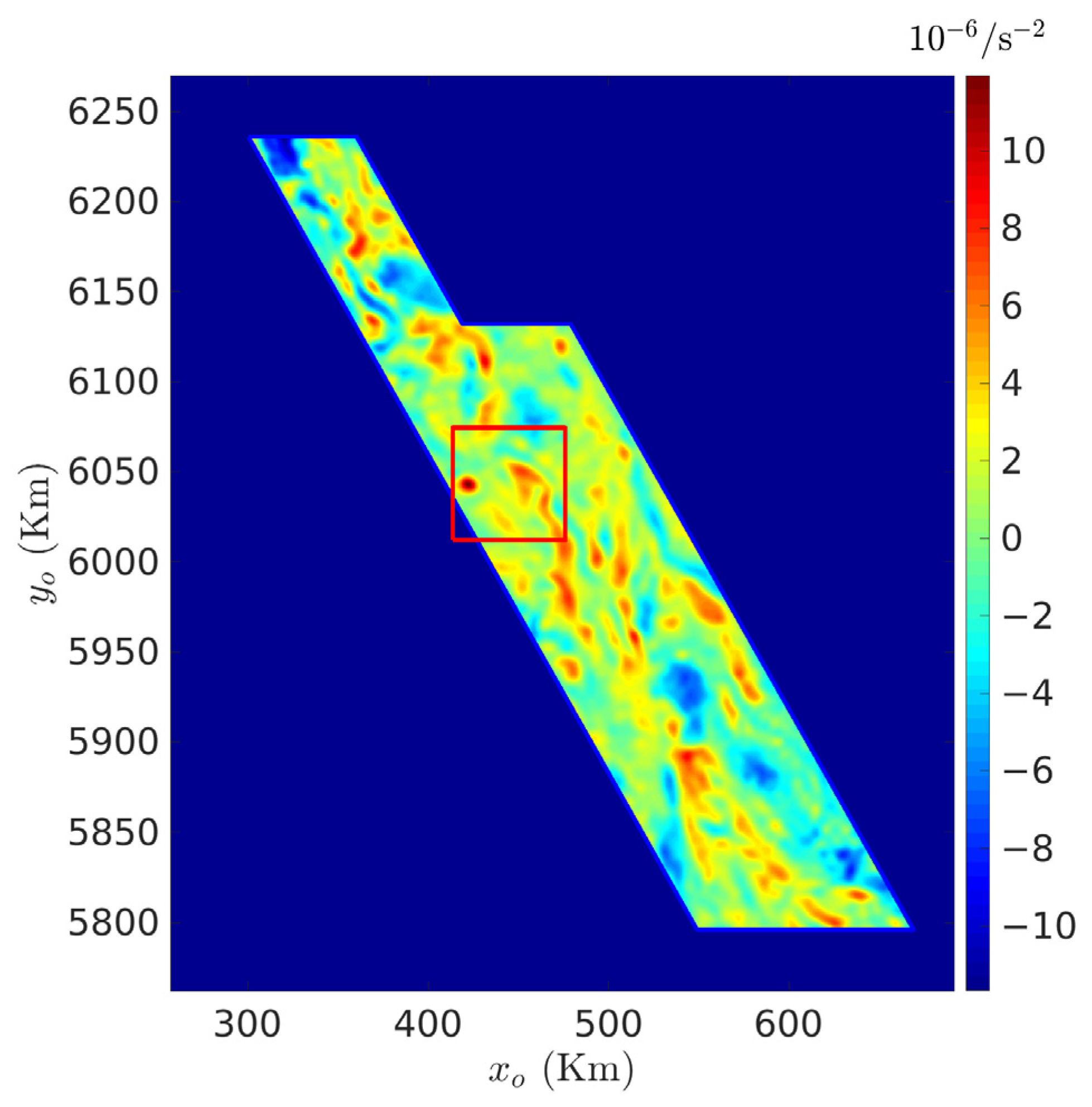
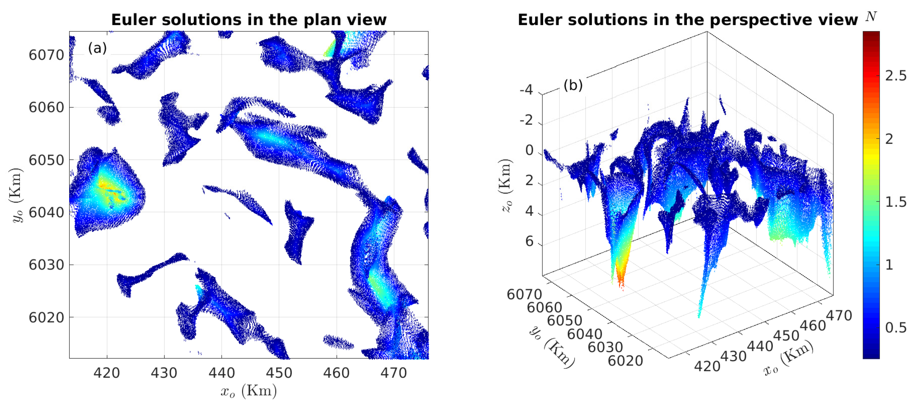
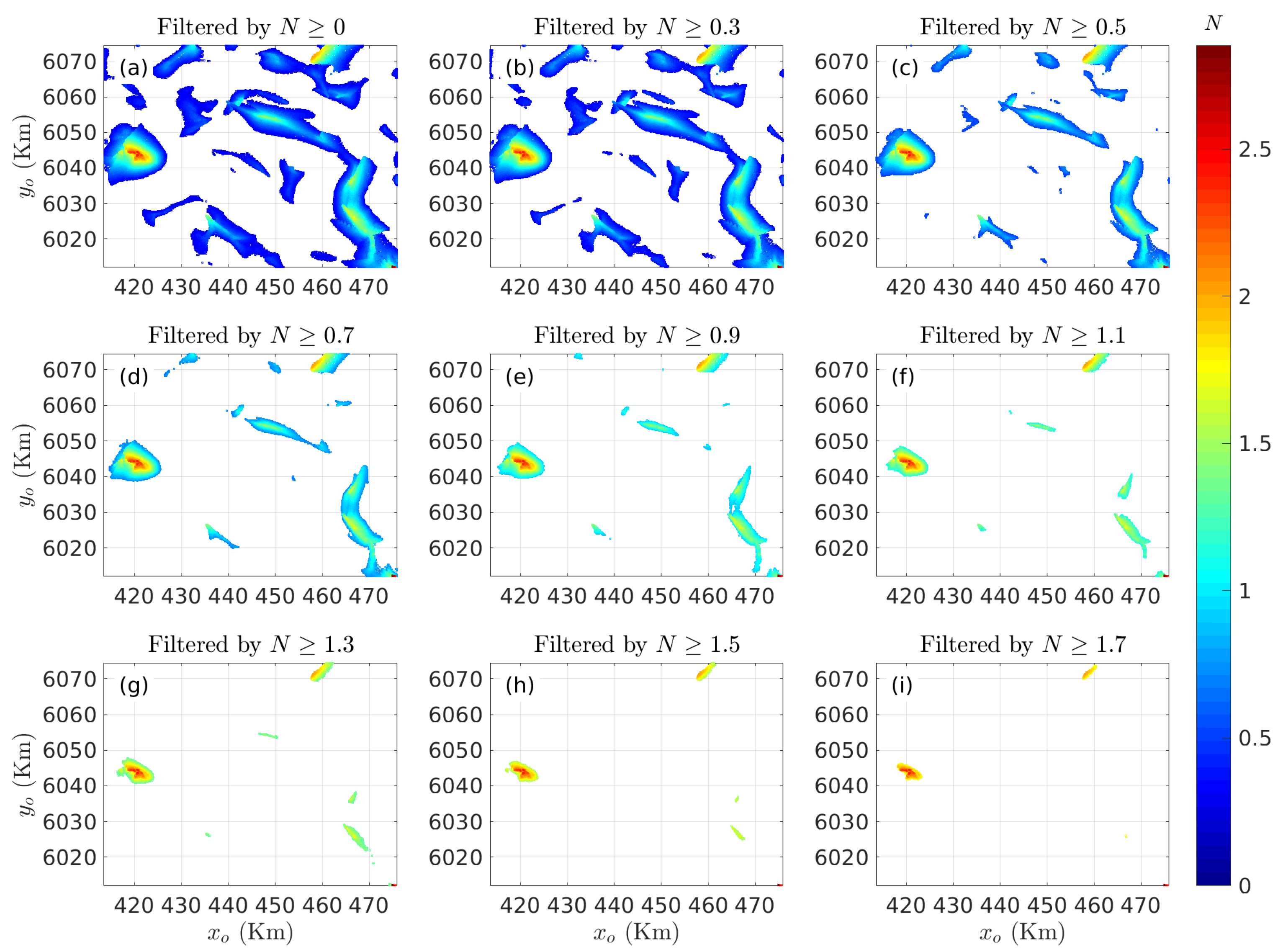
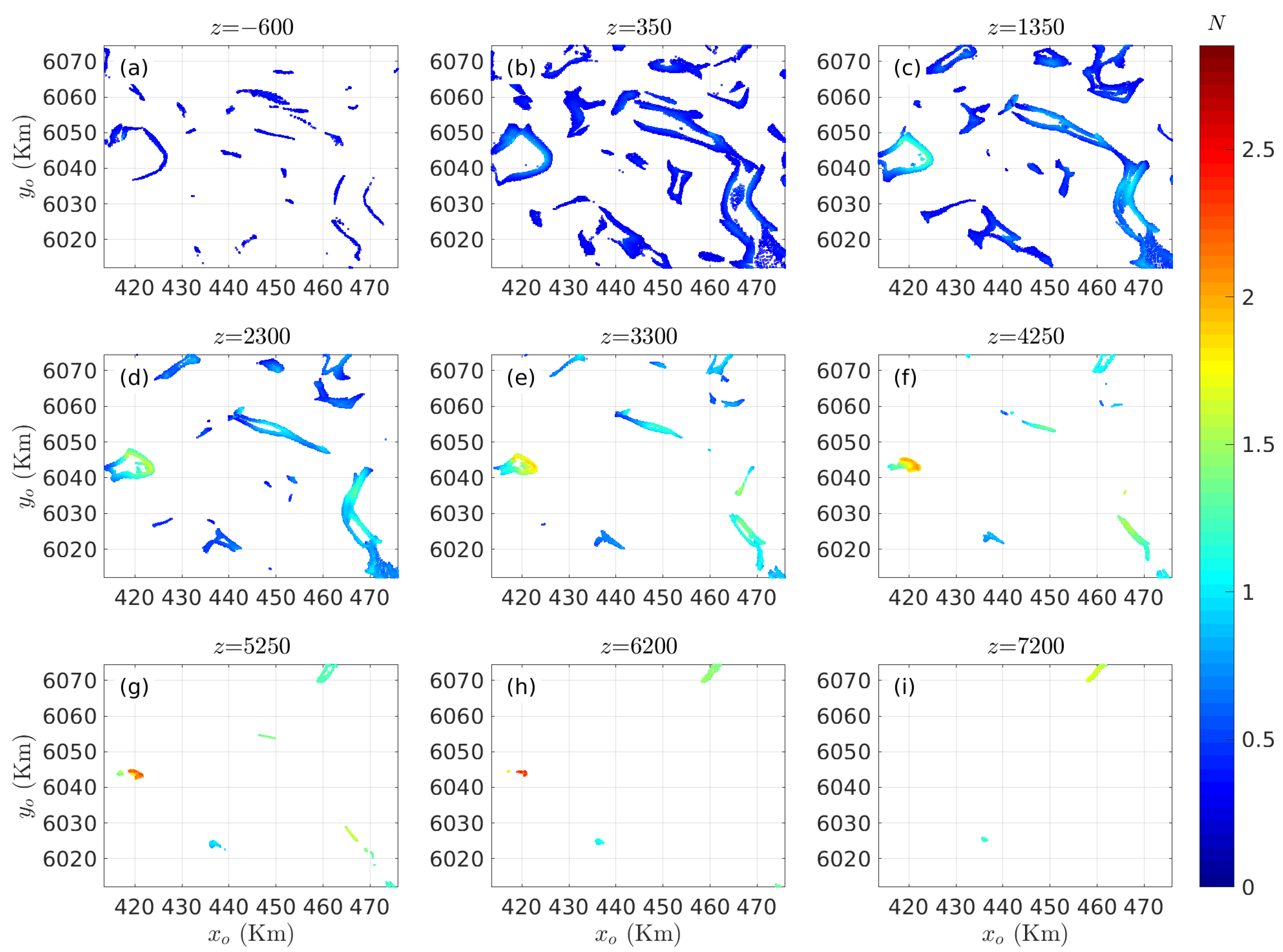
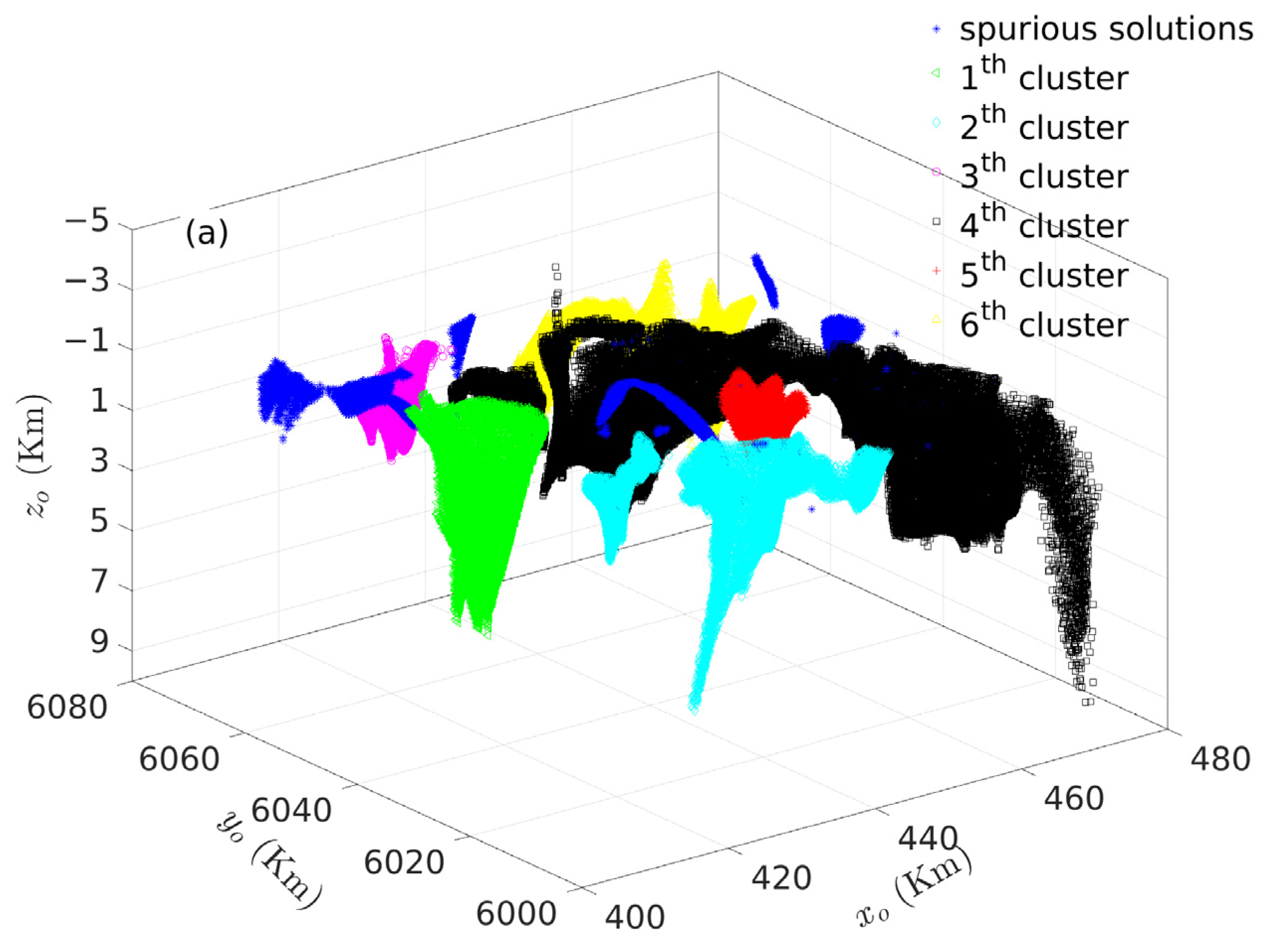
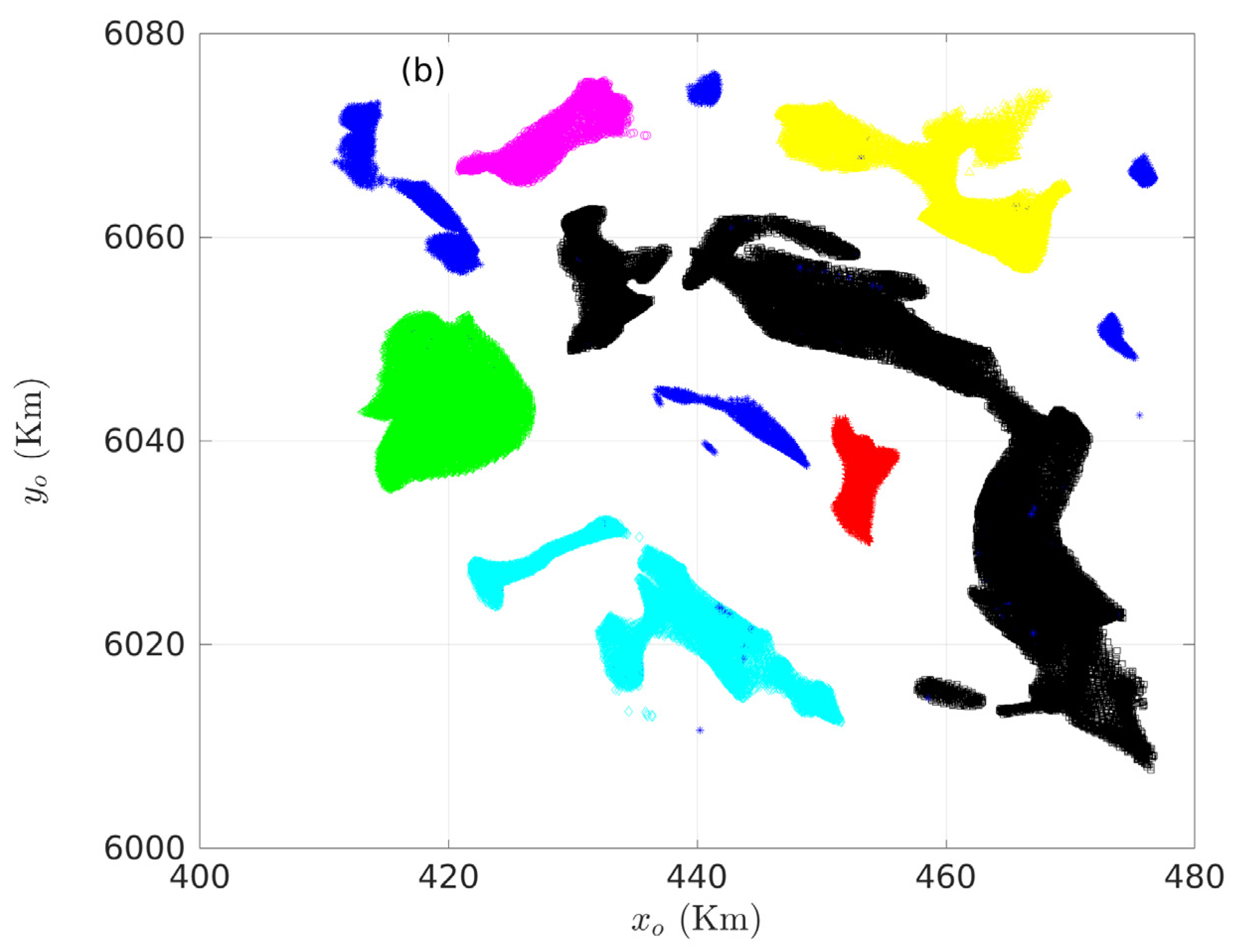
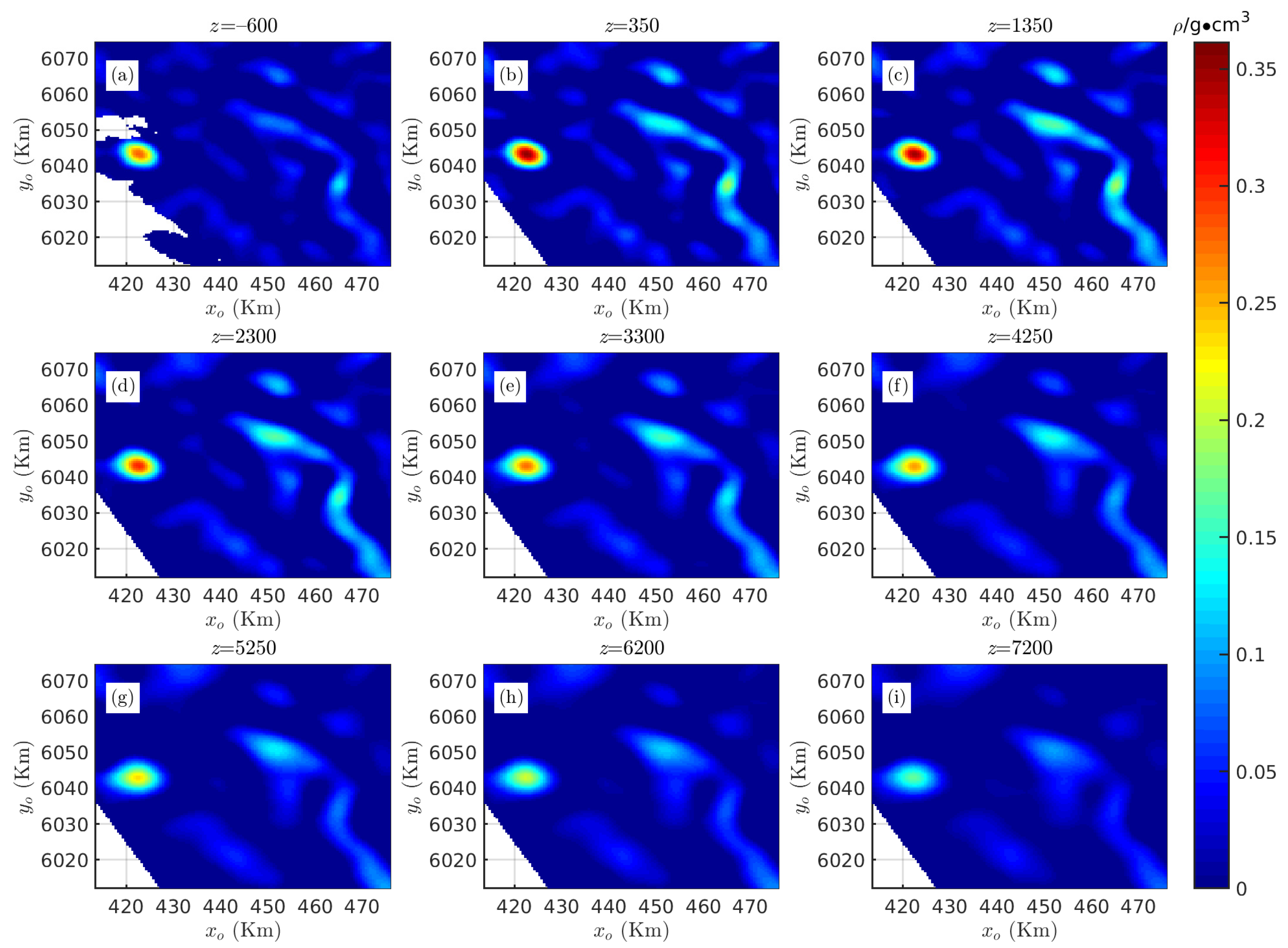
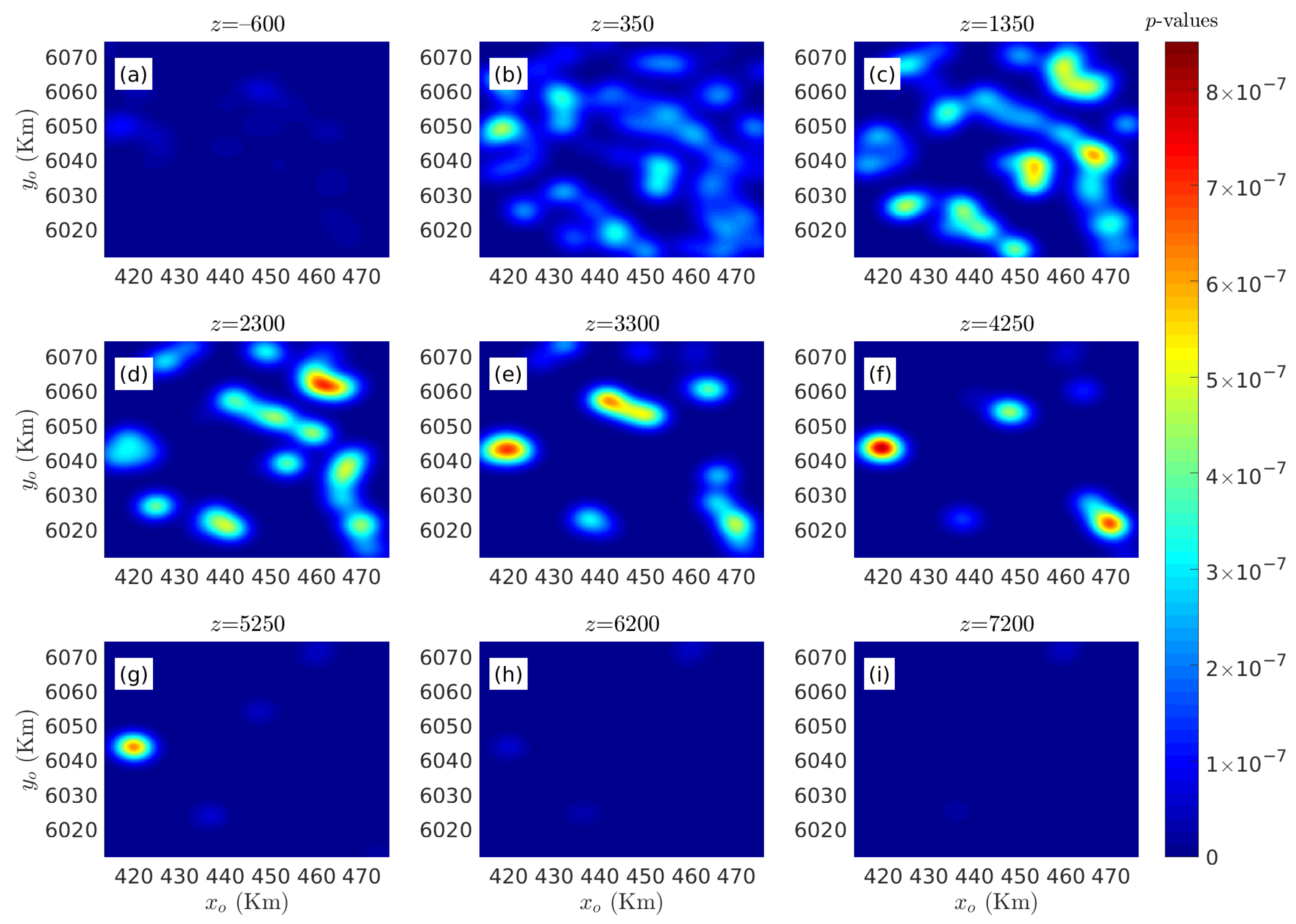
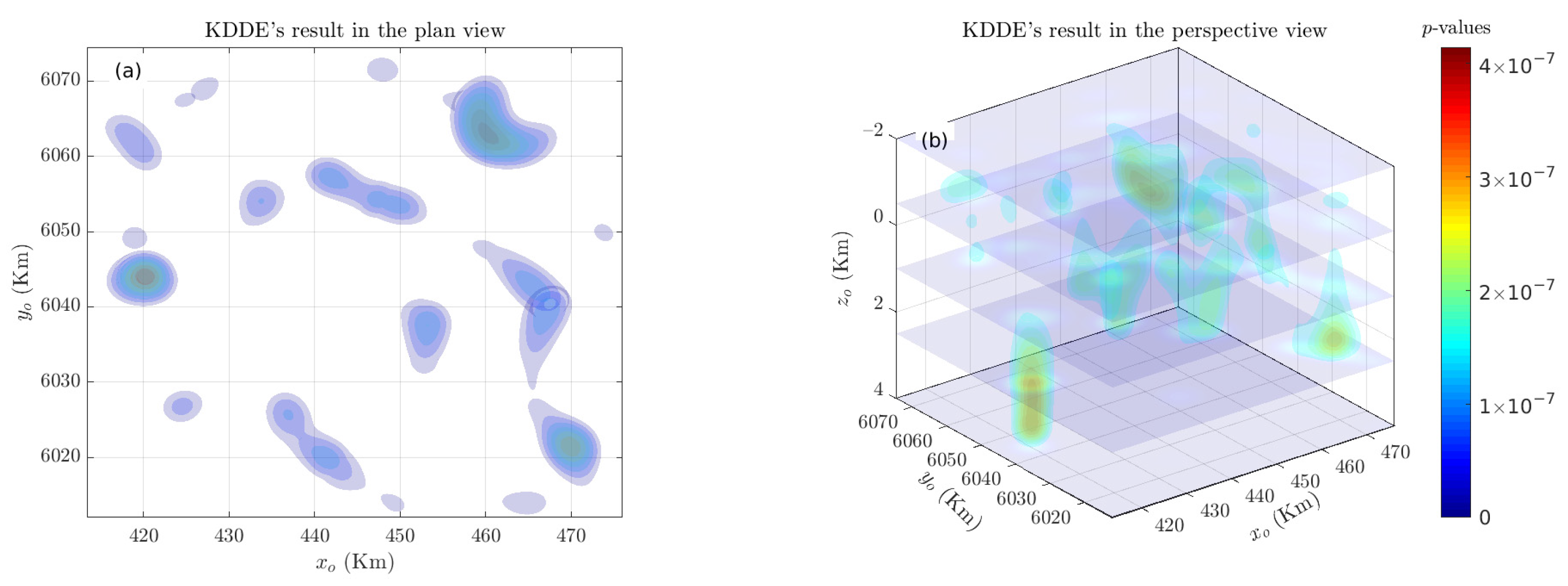
3.2. Case Study in British Columbia, Canada

The survey area was located in the Quesnellia Region in south-central British Columbia, Canada, a region famous for copper and gold porphyry deposits. Several gold and silver (plus copper, lead, and zinc) deposits have been mined in this area since 1884 (Figure 12). The region is covered by a thick layer of sand and gravel left behind by glaciers. Airborne gravity surveys were used to identify potential targets and help understand the geology of this area [91,92]. In our study, the survey block consisted of two connected parallelograms, where the larger one was about 386 km in length and 120 km in width, and the smaller one was 120 km in length and 60 km in width.

Figure 13 shows the construction of gravity data for irregular gravity anomaly data, with a grid size of 250 × 250 m. Figure 13a illustrates the topographic relief contours of the study area, and the measured heights ranged from 717 to 2609 m above the mean sea level. Potential data continuation from an uneven surface to the horizontal planes −2700 m and −5700 m was necessary to obtain the new gravity and background field in Figure 13b. The continuation height corresponding to the background field was determined by the radial average spectrum using Oasis montaj software [93]. The background field was subtracted from the new gravity anomaly to obtain the local gravity anomaly shown in Figure 13c. The FTG data were derived from the local gravity anomaly using the FFT, but only the g_zz component of the FTG is illustrated in Figure 13d.

The entire survey gravity map was covered by a series of moving windows with sizes ranging from 4 × 4 to 12 × 12 data points to form tight clusters of solutions. A total of 2,592,878 solutions were generated using tensor Euler deconvolution before filtering. The Euler solutions are drawn in the plan and perspective views in Figure 14. Difficulties were encountered in separating adjacent clusters of solutions (Figure 14a) and determining the depths of the causative bodies (Figure 14b).

To show the details of the 3-D KDDE results, we selected a small survey grid (red line in Figure 15) with a similar process to that in Figure 14, to yield 155,327 Euler solutions, as shown in Figure 16.

The traditional Euler deconvolution tried to determine the locations of geological targets using a series of tentative N. We used different minimum N and z to filter Euler solutions to simulate this process, as shown in Figure 17 and Figure 18. The scatter plots of the Euler solutions filtered by minimum N (Figure 17) show that the large clusters, especially those in Figure 17d–i, corresponded to the gravity high of g_z in the survey grid in Figure 15. However, it was difficult to determine which cluster corresponds to weak anomalous sources.

The scatter plots of the Euler solutions filtered by different depths (Figure 18) show that multiple-ridge clusters correspond to the boundaries of the gravity high of g_z in the survey grid in Figure 15. However, this correspondence became worse as the depth increases. Therefore, it was difficult to determine which cluster indicated an actual geological body.

If all the clusters are dense enough and are well separated by low-density areas, DBSCAN can find clusters of any shape in the spatial database with “noise” [63,64]. For comparison purposes, we used the DBSCAN to analyze the Euler solutions. The clusters of the Euler solutions (Figure 19) show that the clusters were related to the gravity high of g_z in the survey grid in Figure 15 and the scatter plots of Euler solutions in Figure 17. As the DBSCAN only removed some spurious solutions, there was also no difference between sparse and dense distributions of solutions in the scatter plot compared to other traditional discrimination techniques.

For further comparison, the inversion density distribution maps (Figure 20) were obtained using the UBC-GIF inversion code [94], which was developed based on the Occam’s-style algorithm [95,96]. As surface gravity data had no depth resolution [94] and the Occam’s-style algorithm had difficulty recovering the depth resolution, the density distribution maps became increasingly blurry with the increase of depth z.

Therefore, we used the 3-D KDDE with M = [500, 500, 250] to estimate the Euler solutions (Figure 16) and isolate anomalous sources. We found no probability density contours in Figure 21a, meaning that the spurious solutions, as shown in Figure 17 and Figure 18a, were discriminated by the 3-D KDDE. As the depth z increased from 0.35 to 4.25 km, many probability density contours/ridges appeared, as shown in Figure 21b–f. The contours of probability density images with a higher depth z had high probability values, as shown in Figure 21e–g and their corresponding clusters with larger N values were shown in Figure 18e–h, which confirm each other. These tight clusters with high N shown in Figure 18e–g were discriminated by the 3-D KDDE in Figure 21e–g because they are sparsely located solutions. The other clusters of solutions with lower SIs in Figure 18b–f indicated relatively weaker/smaller geological bodies, as shown in Figure 21b–f.

Figure 22 illustrates the performance of the 3D isosurfaces in estimating the probability density distribution. Figure 16 and Figure 17 show that only using the N to filter spurious solutions made it challenging to determine which clusters of solutions corresponded to actual geological bodies. When lth = 4, the 3D isosurfaces in Figure 22 show that most probability density contours had more meaningful depth resolutions than the Occam’s-style algorithm (Figure 20).

4. Discussion

Spurious solutions may be because of noise, either natural or due to the FFT [32], which was employed to calculate the spatial gradients. This easily produces spurious solutions and yields poor results, especially for potential profile data [24,69].

According to our numerical results, satisfactory probability density distribution results were obtained using 3-D KDDE combined with tensor Euler deconvolution compared to the traditional Euler deconvolution, Euler deconvolution with truncated singular value decomposition [17], and joint Euler deconvolution of gravity gradiometry data [97].

The N is a function of the moving window size and the source-to-observation distance. Consequently, for an arbitrarily shaped source, Euler deconvolution easily yields spurious solutions because no single N is correct at all source-to-observation distances [22]. In addition, using a series of predefined SIs according to a particular step size, the procedure of Euler deconvolution will yield a large number of solutions [25]. To overcome these problems, the N was not predicted in this paper.

Finally, following the suggestions of Reid et al. [69], we proposed a multivariate KDDE approach based on nonparametric estimation to overcome the problem that traditional discrimination techniques are challenging to analyze Euler solutions for visualizing Euler solutions on modern graphics workstations.

For a given Euler solution dataset, the grid size is inversely proportionate to the bandwidth. The bandwidth features a trade-off between the estimator’s bias and its variance. When the bandwidth decreases, the estimated point density has abrupt changes; when it increases, the estimated point density change becomes smoother. The quality of the final probability density distribution of multivariate KDDE is determined by the bandwidth parameters/the grid size. However, if the grid size increases, the computational efficiency of multivariate KDDE with nested for-loops will dramatically decrease. Moreover, when the sample data are combined with high-dimensional sparse data, determining the “best” bandwidth/grid size is time-consuming [62]. The multivariate KDDE, in conjunction with the fast linear binning approximation and the FFT, was proposed with high computational efficiency to overcome this difficulty.

In applying the multivariate KDDE to field data, while the computational efficiency of the multivariate KDDE is essential, we were also concerned with the ability for noise suppression and distinguishing spurious solutions. Hence, based on adjacent anomalous sources with various separations, the results of employing FCM, DBSCAN, and 3-D KDDE were compared and analyzed. Of them, using the probability density contours/isosurfaces of the 3-D KDDE allowed efficient separation of adjacent anomalous sources. Furthermore, the results of the 3-D KDDE for different Gaussian noises indicated that it can effectively separate adjacent anomalous sources and perform consistently, which provides a basis for the application of the multivariate KDDE to complex data. Because of the high-computational efficiency of the multivariate KDDE method, we could try different-sized grids or/and select various lth layer contours to find interesting geological structures more effectively. For example, the 3-D KDDE, in conjunction with the subset {x_o, y_o, z_o} in Figure 16, was carried out with different-sized cubic grids, whose length along one direction was 16, 32, 64, 128, 256, and 512. Its computational time was 0.1109, 0.2552, 0.3581, 1.0352, 7.9938, and 60.4556 s, respectively.

Applying the multivariate KDDE to 1-D or 2-D subsets of Euler solutions yielded too many probability density distribution curves or images, which were challenging to interpret simultaneously. Furthermore, visualization of the 5-D results {x_o, y_o, z_o, N, p-value}, which were obtained by the 4-D KDDE to estimate the entire Euler solution datasets, was very challenging. Although the gplotmatrix function, which plots a matrix with scatter plots by group, can be employed to present high-dimensional data, such as for a simple geological target, it can effectively show characteristics of its locations and SIs. However, applying the gplotmatrix function to analyze complex geological sources is difficult. For this reason, in subsequent research, we will focus on the graphical method of high-dimensional results {x_o, y_o, z_o, N, p-value}.

The 3-D KDDE in conjunction with the subsets {x_o, y_o, z_o}, which derived from the synthetic models and the field data from the survey conducted in British Columbia, Canada, was used to recover more meaningful geological structures than other discrimination techniques successfully.

It is well known that the surface gravity data has no depth resolution [94], and Occam’s -style algorithm is difficult to recover depth resolution. However, the 4-D probability density distribution obtained by our 3-D KDDE method in conjunction with the subsets {x_o, y_o, z_o} derived from tensor Euler deconvolution yielded a higher depth resolution. This is an important finding that will broaden surface gravity data’s application in determining the depths of geological targets.

5. Conclusions

The Geoscience BC project provided the field data used in the study. The residual Bouguer gravity anomaly was the difference between the gravity data continuing upward to −2700 and −5700 m to remove the contributions induced by near-surface. By comparing the results of two clustering methods in Figure 8 and Figure 19 and traditional discriminate techniques in Figure 17 and Figure 18, the results of the multivariate KDDE in conjunction with the subset {x_o, y_o, z_o} obtained using tensor Euler deconvolution were more intuitive and can effectively characterize the geological targets in Figure 9, Figure 21 and Figure 22. In addition, compared to the Occam’s -style algorithm failing to recover the depth resolution from the surface gravity data (Figure 20), our results effectively obtained the depth resolution of the anomalous sources.

In illustrating Euler solutions, because many Euler solutions need to be drawn one by one, the top/newly drawn ones will obscure the bottom/previously drawn ones, whether using a three-dimensional or two-dimensional scatter plot.

Therefore, the multivariate KDDE method of Euler solutions for characterizing geological bodies proposed in this paper contains the following processes: selecting a series of different-sized or fixed-size moving windows, traversing the gridded data using Equation (4) to obtain Euler solutions, constructing an estimation grid with predefined grid size M or bandwidth H, and binning the subset {x_o, y_o, z_o} into the estimation grid via the fast linear binning approximation to yield grid counts c, calculating kernel function evaluations $k$ based on Equation (13), constructing the zero-padded versions of the grid count $C$ and the kernel evaluation $K$, and carrying out the convolution between $C$ and $K$ quickly by FFT to get the probability density distribution of the subset {x_o, y_o, z_o}.

Tests on the field data showed that the multivariate KDDE, which was used in conjunction with the subset {x_o, y_o, z_o} obtained using tensor Euler deconvolution, proposed in this paper, does not rely on a priori geological information. Therefore, it is suitable for analyzing and interpreting large-area potential field data. In addition, the depth resolution information extracted from the surface gravity data using 3-D KDDE can be used as a constraint to analyze geological targets. Consequently, the ideal geological targets would be compact three-dimensional bodies with sharp boundaries, such as salt domes, ore bodies, and igneous intrusions.

The estimated grid size is proportional to the bandwidth size for a given input data instance. Therefore, only one parameter, H or M, was required in the manuscript regarding the multivariate KDDE to process the sample data. Regarding the analysis of the multivariate KDDE of the field data, the required data and parameters were g_z, w_x, w_y, H, or M.

References

1. Ugalde, H.; Morris, W. Deriving geological contact geometry from potential field data. Explor. Geophys. 2010, 41, 40–50. [Google Scholar] [CrossRef]
2. Zheng, S.; Meng, X.; Wang, J. An edge-assisted smooth method for potential field data. J. Geophys. Eng. 2021, 18, 113–123. [Google Scholar] [CrossRef]
3. Bertete-Aguirre, H.; Cherkaev, E.; Oristaglio, M. Non-smooth gravity problem with total variation penalization functional. Geophys. J. Int. 2002, 149, 499–507. [Google Scholar] [CrossRef] [Green Version]
4. Namaki, L.; Gholami, A.; Hafizi, M.A. Edge-preserved 2-D inversion of magnetic data: An application to the Makran arc-trench complex. Geophys. J. Int. 2011, 184, 1058–1068. [Google Scholar] [CrossRef] [Green Version]
5. Zhdanov, M.S.; Ellis, R.; Mukherjee, S. Three-dimensional regularized focusing inversion of gravity gradient tensor component data. Geophysics 2004, 69, 925–937. [Google Scholar] [CrossRef]
6. DiFrancesco, D.; Grierson, A.; Kaputa, D.; Meyer, T. Gravity gradiometer systems—Advances and challenges. Geophys. Prospect. 2009, 57, 615–623. [Google Scholar] [CrossRef]
7. Zhu, Z.; Wang, C.; Lu, G.; CAO, S. Euler deconvolution of analytic signals of gravity gradient tensor. J. Cent. South Univ. (Sci. Technol.) (Chin.) 2015, 46, 217–222. [Google Scholar]
8. Pan, Q.; Liu, D.; Feng, S.; Feng, M.; Fang, H. Euler deconvolution of the analytic signals of the gravity gradient tensor for the horizontal pipeline of finite length by horizontal cylinder calculation. J. Geophys. Eng. 2017, 14, 316–330. [Google Scholar] [CrossRef] [Green Version]
9. Thompson, D. EULDPH: A new technique for making computer-assisted depth estimates from magnetic data. Geophysics 1982, 47, 31–37. [Google Scholar] [CrossRef]
10. Reid, A.; Allsop, J.; Granser, H.; Millett, A.; Somerton, I. Magnetic interpretation in three dimensions using Euler deconvolution. Geophysics 1990, 55, 80–91. [Google Scholar] [CrossRef] [Green Version]
11. Hearst, R.; Morris, W. Interpretation of the Sudbury structure through Euler deconvolution. In SEG Technical Program Expanded Abstracts 1993; Society of Exploration Geophysicists: Washington, DC, USA, 1993; pp. 421–424. [Google Scholar]
12. Silva, J.B.C.; Barbosa, V.C.F. 3D Euler deconvolution: Theoretical basis for automatically selecting good solutions. Geophysics 2003, 68, 1962–1968. [Google Scholar] [CrossRef]
13. Keating, P.; Pilkington, M. Euler deconvolution of the analytic signal and its application to magnetic interpretation. Geophys. Prospect. 2004, 52, 165–182. [Google Scholar] [CrossRef]
14. Gerovska, D.; Araúzo-Bravo, M.J. Automatic interpretation of magnetic data based on Euler deconvolution with unprescribed structural index. Comput. Geosci. 2003, 29, 949–960. [Google Scholar] [CrossRef]
15. Nabighian, M.; Hansen, R. Unification of Euler and Werner deconvolution in three dimensions via the generalized Hilbert transform. Geophysics 2001, 66, 1805–1810. [Google Scholar] [CrossRef] [Green Version]
16. Stavrev, P.; Reid, A. Euler deconvolution of gravity anomalies from thick contact/fault structures with extended negative structural index. Geophysics 2010, 75, I51–I58. [Google Scholar] [CrossRef]
17. Beiki, M. TSVD analysis of Euler deconvolution to improve estimating magnetic source parameters: An example from the Åsele area, Sweden. J. Appl. Geophys. 2013, 90, 82–91. [Google Scholar] [CrossRef]
18. Wang, J.; Meng, X.; Li, F. New improvements for lineaments study of gravity data with improved Euler inversion and phase congruency of the field data. J. Appl. Geophys. 2017, 136, 326–334. [Google Scholar] [CrossRef]
19. Dewangan, P.; Ramprasad, T.; Ramana, M.V.; Desa, M.; Shailaja, B. Automatic interpretation of magnetic data using Euler deconvolution with nonlinear background. Pure Appl. Geophys. 2007, 164, 2359–2372. [Google Scholar] [CrossRef] [Green Version]
20. Ekinci, Y.L.; Balkaya, Ç.; Şeren, A.; Kaya, M.A.; Lightfoot, C.S. Geomagnetic and geoelectrical prospection for buried archaeological remains on the Upper City of Amorium, a Byzantine city in midwestern Turkey. J. Geophys. Eng. 2014, 11, 015012. [Google Scholar] [CrossRef]
21. Rabeh, T.; Khalil, A. Characterization of fault structures in southern Sinai Peninsula and Gulf of Suez region using geophysical data. Environ. Earth Sci. 2015, 73, 1925–1937. [Google Scholar] [CrossRef]
22. Ravat, D. Analysis of the Euler Method and Its Applicability in Environmental Magnetic Investigations. J. Environ. Eng. Geophys. 1996, 1, 229–238. [Google Scholar] [CrossRef]
23. Hsu, S.K. Imaging magnetic sources using Euler’s equation. Geophys. Prospect. 2002, 50, 15–25. [Google Scholar] [CrossRef]
24. Melo, F.F.; Barbosa, V.C.F. What to expect from Euler deconvolution estimates for isolated sources. In Proceedings of the 15th International Congress of the Brazilian Geophysical Society & EXPOGEF, Rio de Janeiro, Brazil, 31 July–3 August 2017; pp. 1092–1097. [Google Scholar]
25. Mikhailov, V.; Pajot, G.; Diament, M.; Price, A. Tensor deconvolution: A method to locate equivalent sources from full tensor gravity data. Geophysics 2007, 72, I61–I69. [Google Scholar] [CrossRef] [Green Version]
26. Cooper, G. Iterative Euler deconvolution. Explor. Geophys. 2021, 52, 468–474. [Google Scholar] [CrossRef]
27. Beiki, M. Analytic signals of gravity gradient tensor and their application to estimate source location. Geophysics 2010, 75, I59–I74. [Google Scholar] [CrossRef]
28. Wang, M.; Guo, Z.; Luo, Y.; Luo, F.; Guo, H.; Qu, J. The application of Tilt-Euler deconvolution method to potential field data processing and interpretation. Geophys. Geochem. Explor. (Chin.) 2012, 36, 126–132. [Google Scholar]
29. Florio, G.M.R. On the application of Euler deconvolution to the analytic signal. Geophysics 2006, 71, L87–L93. [Google Scholar] [CrossRef] [Green Version]
30. Reid, A.B.; Thurston, J.B. The structural index in gravity and magnetic interpretation: Errors, uses, and abuses. Geophysics 2014, 79, J61–J66. [Google Scholar] [CrossRef]
31. Zhou, W.; Nan, Z.; Li, J. Self-constrained Euler deconvolution using potential field data of different altitudes. Pure Appl. Geophys. 2016, 173, 2073–2085. [Google Scholar] [CrossRef]
32. Farrelly, B. What is Wrong with Euler Deconvolution? In Proceedings of the 59th EAGE Conference & Exhibition. Geneva, Switzerland, 26–30 May 1997; p. cp-131-00225. [Google Scholar] [CrossRef]
33. Zhang, C.; Mushayandebvu, M.; Reid, A.; Fairhead, J.; Odegard, M. Euler deconvolution of gravity tensor gradient data. Geophysics 2000, 65, 512–520. [Google Scholar] [CrossRef] [Green Version]
34. FitzGerald, D.; Reid, A.; McInerney, P. New discrimination techniques for Euler deconvolution. Comput. Geosci. 2004, 30, 461–469. [Google Scholar] [CrossRef]
35. Reid, A.B.; Ebbing, J.; Webb, S.J. Avoidable Euler errors—The use and abuse of Euler deconvolution applied to potential fields. Geophys. Prospect. 2014, 62, 1162–1168. [Google Scholar] [CrossRef]
36. Silva, J.; Barbosa, V.; Medeiros, W. Scattering, symmetry, and bias analysis of source-position estimates in Euler deconvolution and its practical implications. Geophysics 2001, 66, 1149–1156. [Google Scholar] [CrossRef]
37. Li, X. On the use of different methods for estimating magnetic depth. Lead. Edge 2003, 22, 1090–1099. [Google Scholar] [CrossRef]
38. Barbosa, V.C.; Silva, J.B.; Medeiros, W.E. Stability analysis and improvement of structural index estimation in Euler deconvolution. Geophysics 1999, 64, 48–60. [Google Scholar] [CrossRef]
39. Fedi, M. DEXP: A fast method to determine the depth and the structural index of potential fields sources. Geophysics 2007, 72, I1. [Google Scholar] [CrossRef]
40. Melo, F.F.; Barbosa, V.C. Correct structural index in Euler deconvolution via base-level estimates. Geophysics 2018, 83, J87–J98. [Google Scholar] [CrossRef]
41. Huang, L.; Zhang, H.; Sekelani, S.; Wu, Z. An improved Tilt-Euler deconvolution and its application on a Fe-polymetallic deposit. Ore Geol. Rev. 2019, 114, 103114. [Google Scholar] [CrossRef]
42. Salem, A.; Ravat, D. A combined analytic signal and Euler method (AN-EUL) for automatic interpretation of magnetic data. Geophysics 2003, 68, 1952–1961. [Google Scholar] [CrossRef]
43. Salem, A.; Ravat, D.; Smith, R.; Ushijima, K. Interpretation of magnetic data using an enhanced local wavenumber (ELW) method. Geophysics 2005, 70, L7–L12. [Google Scholar] [CrossRef]
44. Salem, A.; Williams, S.; Fairhead, D.; Smith, R.; Ravat, D. Interpretation of magnetic data using tilt-angle derivatives. Geophysics 2008, 73, L1–L10. [Google Scholar] [CrossRef]
45. Ma, G. Combination of horizontal gradient ratio and Euler (HGR-EUL) methods for the interpretation of potential field data. Geophysics 2013, 78, J53–J60. [Google Scholar] [CrossRef]
46. Cooper, G.R.; Whitehead, R.C. Determining the distance to magnetic sources. Geophys. J. Soc. Explor. Geophys. 2016, 81, J25–J34. [Google Scholar] [CrossRef]
47. Cooper, G.R.J. Determining the depth and location of potential field sources without specifying the structural index. Arab. J. Geosci. 2017, 10, 438. [Google Scholar] [CrossRef]
48. Yao, C.; Guan, Z.; Wu, Q.; Ahang, Y.; Liu, H. An analysis of Euler deconvolution and its improvement. Geophys. Geochem. Explor. (Chin.) 2004, 28, 150–155. [Google Scholar]
49. Sanchez-Rojas, J.; Palma, M. Crustal density structure in northwestern South America derived from analysis and 3-D modeling of gravity and seismicity data. Tectonophysics 2014, 634, 97–115. [Google Scholar] [CrossRef]
50. Mikhailov, V.; Galdeano, A.; Diament, M.; Gvishiani, A.; Agayan, S.; Bogoutdinov, S.; Graeva, E.; Sailhac, P. Application of artificial intelligence for Euler solutions clustering. Geophysics 2003, 68, 168–180. [Google Scholar] [CrossRef] [Green Version]
51. Gvishiani, A.D.; Mikhailov, V.O.; Agayan, S.M.; Bogoutdinov, S.R.; Graeva, E.M.; Diament, M.; Galdeano, A. Artificial intelligence algorithms for magnetic anomaly clustering. Izv. Phys. Solid Earth 2002, 38, 545–559. [Google Scholar] [CrossRef]
52. Husson, E.; Guillen, A.; Séranne, M.; Courrioux, G.; Couëffé, R. 3D Geological modelling and gravity inversion of a structurally complex carbonate area: Application for karstified massif localization. Basin Res. 2018, 30, 766–782. [Google Scholar] [CrossRef] [Green Version]
53. Lee, J.-H.; Kim, D.-H.; Chung, C.-W. Multi-dimensional selectivity estimation using compressed histogram information. SIGMOD Rec. 1999, 28, 205–214. [Google Scholar] [CrossRef]
54. Dal Moro, G.; Pipan, M.; Gabrielli, P. Rayleigh wave dispersion curve inversion via genetic algorithms and marginal posterior probability density estimation. J. Appl. Geophys. 2007, 61, 39–55. [Google Scholar] [CrossRef]
55. Trainor-Guitton, W.; Hoversten, G.M. Stochastic inversion for electromagnetic geophysics: Practical challenges and improving convergence efficiency. Geophysics 2011, 76, F373–F386. [Google Scholar] [CrossRef]
56. Boschetti, F.; Hornby, P.; Horowitz, F.G. Wavelet based inversion of gravity data. Explor. Geophys. 2001, 32, 48–55. [Google Scholar] [CrossRef]
57. Fregoso, E.; Palafox, A.; Moreles, M.A. Initializing cross-gradients joint inversion of gravity and magnetic data with a Bayesian surrogate gravity model. Pure Appl. Geophys. 2020, 177, 1029–1041. [Google Scholar] [CrossRef]
58. Bosch, M.; Meza, R.; Jiménez, R.; Hönig, A. Joint gravity and magnetic inversion in 3D using Monte Carlo methods. Geophysics 2006, 71, G153–G156. [Google Scholar] [CrossRef]
59. Ekinci, Y.L.; Balkaya, Ç.; GÖKtÜRkler, G. Parameter estimations from gravity and magnetic anomalies due to deep-seated faults: Differential evolution versus particle swarm optimization. Turk. J. Earth Sci. 2019, 28, 860–881. [Google Scholar] [CrossRef]
60. Bosch, M.; McGaughey, J. Joint inversion of gravity and magnetic data under lithologic constraints. Lead. Edge 2001, 20, 877–881. [Google Scholar] [CrossRef] [Green Version]
61. Sheather, S.J. Density estimation. Stat. Sci. 2004, 19, 588–597. [Google Scholar] [CrossRef]
62. Duong, T.; Cowling, A.; Koch, I.; Wand, M.P. Feature significance for multivariate kernel density estimation. Comput. Stat. Data Anal. 2008, 52, 4225–4242. [Google Scholar] [CrossRef]
63. Ester, M.; Kriegel, H.-P.; Sander, J.O.R.; Xu, X. A Density-Based Algorithm for Discovering Clusters in Large Spatial Databases with Noise. In Proceedings of the Second International Conference on Knowledge Discovery and Data Mining, Portland, OR, USA, 2–4 August 1996; pp. 226–231. [Google Scholar] [CrossRef]
64. Daszykowski, M.; Walczak, B.; Massart, D.L. Looking for natural patterns in data. Chemom. Intell. Lab. Syst. 2001, 56, 83–92. [Google Scholar] [CrossRef]
65. Ugalde, H.; Morris, W. Cluster analysis of Euler deconvolution solutions: New filtering techniques and geologic strike determination. Geophysics 2010, 75, L61–L70. [Google Scholar] [CrossRef]
66. Michel, H.; Nguyen, F.; Kremer, T.; Elen, A.; Hermans, T. 1D geological imaging of the subsurface from geophysical data with Bayesian Evidential Learning. Comput. Geosci. 2020, 138, 104456. [Google Scholar] [CrossRef]
67. Eckert-Gallup, A.; Martin, N. Kernel density estimation (KDE) with adaptive bandwidth selection for environmental contours of extreme sea states. In Proceedings of the OCEANS 2016 MTS/IEEE Monterey, Monterey, CA, USA, 19–23 September 2016; pp. 1–5. [Google Scholar] [CrossRef]
68. Allsop, J.M.; Evans, C.J.; McDonald, A.J.W. Visualizing and interpreting 3-D Euler solutions using enhanced computer graphics. Surv. Geophys. 1991, 12, 553–564. [Google Scholar] [CrossRef]
69. Reid, A.B. Euler deconvolution: Past, present and future—A review. In Proceedings of the 65th SEG Meeting, Houston, TX, USA, 8–13 October 1995; pp. 272–273. [Google Scholar] [CrossRef] [Green Version]
70. Gramacki, A. Nonparametric Kernel Density Estimation and Its Computational Aspects: Studies in Big Data; Springer: Cham, Switzerland, 2018; Volume 37, pp. 58–59. [Google Scholar]
71. Grana, D.; Della Rossa, E. Probabilistic petrophysical-properties estimation integrating statistical rock physics with seismic inversion. Geophysics 2010, 75, O21–O37. [Google Scholar] [CrossRef]
72. Buland, A.; Kolbjørnsen, O.; Hauge, R.; Skjæveland, Ø.; Duffaut, K. Bayesian lithology and fluid prediction from seismic prestack data. Geophysics 2008, 73, C13–C21. [Google Scholar] [CrossRef]
73. Zhou, W.-Y.; Ma, G.-Q.; Hou, Z.-L.; Qin, P.-B.; Meng, Z.-H. The study on the joint Euler deconvolution method of full tensor gravity data. Chin. J. Geophys. (Chin.) 2017, 60, 4855–4865. [Google Scholar] [CrossRef]
74. Florio, G.; Fedi, M. Multiridge euler deconvolution. Geophys. Prospect. 2014, 62, 333–351. [Google Scholar] [CrossRef] [Green Version]
75. Scott, D.W. Multivariate Density Estimation: Theory, Practice, and Visualization; John Wiley & Sons: Hoboken, NJ, USA, 2015; pp. 161–167. [Google Scholar]
76. Chacón, J.E.; Duong, T. Multivariate Kernel Smoothing and Its Applications; CRC Press: Boca Raton, FL, USA, 2018; pp. 185–190. [Google Scholar]
77. Gramacki, A.; Gramacki, J. FFT-Based Fast Computation of Multivariate Kernel Density Estimators With Unconstrained Bandwidth Matrices. J. Comput. Graph. Stat. 2017, 26, 459–462. [Google Scholar] [CrossRef]
78. Guidoum, A.C. Kernel Estimator and Bandwidth Selection for Density and Its Derivatives. The Kedd Package, Version 1.03, October 2015. Available online: https://rdrr.io/cran/kedd/f/inst/doc/kedd.pdf (accessed on 28 January 2023).
79. Van Kerm, P. Adaptive kernel density estimation. Stata J. 2003, 3, 148–156. [Google Scholar] [CrossRef]
80. Wand, M.P. Fast computation of multivariate kernel estimators. J. Comput. Graph. Stat. 1994, 3, 433–445. [Google Scholar] [CrossRef]
81. González-Manteiga, W.; Sánchez-Sellero, C.; Wand, M.P. Accuracy of binned kernel functional approximations. Comput. Stat. Data Anal. 1996, 22, 1–16. [Google Scholar] [CrossRef]
82. Silverman, B.W. Density Estimation for Statistics and Data Analysis; Chapman and Hall: New York, NY, USA, 1986; pp. 61–65. [Google Scholar]
83. Rao, S. Interpolation Models. In The Finite Element Method in Engineering, 6th ed.; Butterworth-Heinemann: Oxford, UK, 2017; pp. 81–127. [Google Scholar] [CrossRef]
84. Cook, S.A.; Aanderaa, S.O. On the minimum computation time of functions. Trans. Am. Math. Soc. 1969, 142, 291–314. [Google Scholar] [CrossRef]
85. Agarwal, R.; Cooley, J.W. New algorithms for digital convolution. IEEE Trans. Acoust. Speech Signal Process. 1977, 25, 392–410. [Google Scholar] [CrossRef]
86. Winograd, S. Arithmetic Complexity of Computations; SIAM: Philadelphia, PA, USA, 1980; Volume 33. [Google Scholar] [CrossRef]
87. Teukolsky, S.A.; Flannery, B.P.; Press, W.H.; Vetterling, W.T. Numerical Recipes in C: The Art of Scientific Computing; Cambridge University Press: Cambridge, UK, 1992. [Google Scholar] [CrossRef] [Green Version]
88. Arndt, J. Matters Computational: Ideas, Algorithms, Source Code; Springer Science & Business Media: Berlin/Heidelberg, Germany, 2010. [Google Scholar]
89. Mikhailov, V.O.; Diament, M. Some aspects of interpretation of tensor gradiometry data. Izv. Phys. Solid Earth 2006, 42, 971–978. [Google Scholar] [CrossRef]
90. Pašteka, R.; Kušnirák, D.; Götze, H.J. Stabilization of the Euler deconvolution algorithm by means of a two steps regularization approach. In Proceedings of the EGM 2010 International Workshop, Capri, Italy, 11–14 April 2010; p. cp-165-00058. [Google Scholar] [CrossRef]
91. Phillips, N.; Thi, N.H.N.; Thomson, V.; Mira, G.A.G.I. 3D inversion modelling, integration, and visualization of airborne gravity, magnetic, and electromagnetic data: The Quest Project. Geosci. BC Rep. 2009, 2009–2015. [Google Scholar] [CrossRef]
92. Reichheld, S.A. Documentation and Assessment of Exploration Activities Generated by Geoscience BCData Publications, QUEST Project, Central British Columbia (NTS 093A, B, G, H, J, K, N, O, 094C, D); Geoscience BC: Vancouver, BC, Canada, 2013; pp. 125–130. [Google Scholar]
93. Montaj, G.O. The Core Software Platform for Working with Large Volume Gravity and Magnetic Spatial Data; Geosoft Inc.: Toronto, ON, Canada, 2008. [Google Scholar]
94. Li, Y.; Oldenburg, D. 3-D inversion of gravity data. Geophysics 1998, 63, 109–119. [Google Scholar] [CrossRef]
95. LaBrecque, D.J.; Owen, E.; Dailey, W.; Ramirez, A.L. Noise and occam’s inversion of resistivity tomography data. In SEG Technical Program Expanded Abstracts 1992; Society of Exploration Geophysicists: New Orleans, LA, USA, 1992; pp. 397–400. [Google Scholar] [CrossRef]
96. Siripunvaraporn, W.; Sarakorn, W. An efficient data space conjugate gradient Occam’s method for three-dimensional magnetotelluric inversion. Geophys. J. Int. 2011, 186, 567–579. [Google Scholar] [CrossRef] [Green Version]
97. Hou, Z.-L.; Wang, E.-D.; Zhou, W.-N.; Wu, G.-C. Euler deconvolution of gravity gradiometry data and the application in Vinton Dome. Oil Geophys. Prospect. (Chin.) 2019, 54, 472–479+242. [Google Scholar] [CrossRef]
Figure 1. Linear binning counts. (a) A univariate data X i is converted to the counts assigned to its 2 nearest grid points χ j and χ j + 1 . Their respective counts are equal to the length of the opposite line segment divided by the total length of bin A. (b) A bivariate data X i is converted to the counts assigned to its four nearest grid points. Following Rao’s book [83] and Chacón and Duong’s book [76], their respective counts are equal to their natural coordinate value. Reprinted with permission from Ref. [76]. Copyright 2018 Taylor & Francis Group LLC.
Applsci 13 01784 g001
Figure 2. Computation times of the Brute-Force algorithm and the fast linear binning approximation according to the number of sample data n and the grid size M.
Applsci 13 01784 g002
Figure 3. Computation times of the 1-D KDDE were calculated using the FFT and nested for-loops according to the grid size M and the number of sample data n.
Applsci 13 01784 g003
Figure 4. Scatter plots of the Euler solutions. (a,b) Contours of noise-free gravity. (c,d) Euler solutions derived from noise-free FTG. (e,f) Euler solutions derived from noise-corrupted FTG. (g,h) Euler solutions for noise-corrupted FTG in the plan view, for the cube and the cylinder, whose frames are solid black.
Applsci 13 01784 g004
Figure 5. Histograms of the N of Euler solutions derived from: (a) noise-free gravity data; (b) noise-corrupted gravity data of the cube model; (c) noise-free gravity data; and (d) noise-corrupted gravity data of the cylinder. The width of each bin for N is 0.025.
Applsci 13 01784 g005
Figure 6. Probability density curves obtained using 1-D kernel density derivative estimate (KDDE) with M = 100 for the subsets: (a) {xo}, (b) {yo}, (c) {zo}, and (d) {N}, of the cube and cylinder models, with n = 6700 and 7227, respectively.
Applsci 13 01784 g006
Figure 7. Probability density isosurfaces obtained using the 3-D KDDE for the subset {xo, yo, zo}. Where (a) lth = 1 and (b) lth = 2 are for the cube; (c) lth = 1 and (d) lth = 2 are for the cylinder. w x = w y = 5 . M = [100, 100, 100].
Applsci 13 01784 g007
Figure 8. Clustering methods were used to separate the adjacent clusters formed by Euler solutions. (a–c) Contours of contaminated gravity. (df) The Euler solutions derived from the contaminated FTG with w x = w y = 15 . (gi) Clusters of Euler solutions got by the FCM algorithm, which initializes with two random clusters and the minimum improvement is 10−5. (jl) Clusters of Euler solutions got by the density-based spatial clustering of applications with noise (DBSCAN) algorithm yields three clusters, and the object numbers of their neighborhood are 61, 70 and 72, respectively. Their neighborhood radii are 238.62 m, 222.97 m, and 238.22 m, respectively.
Applsci 13 01784 g008
Figure 9. Probability density isosurfaces obtained using the 3-D KDDE for the subset {xo, yo, zo} with varied separations: (a) 4.0 km; (b) 2.5 km; and (c) 1.0 km. M = [100, 100, 100]. w x = w y = 15 . lth = 2.
Applsci 13 01784 g009
Figure 10. Illustration of 3-D KDDE of sensitivity to different Gaussian noises: in the top, middle, and bottom row is p = 0, 4, and 8, respectively. w x = w y = 7, n = 8849, M = [300, 300, 200], and lth = 5.
Applsci 13 01784 g010
Figure 11. Probability density distribution obtained using 3-D KDDE with different-sized grid: (a) 16 × 16 × 16; (b) 32 × 32 × 32; (c) 64 × 64 × 64; (d) 128 × 128 × 128; (e) 256 × 256 × 256; (f) 512 × 512 × 512. w x = w y = 7, and lth = 5.
Applsci 13 01784 g011
Figure 12. Locations map.
Applsci 13 01784 g012
Figure 13. Construction of FTG data for irregular gravitational anomaly data. (a) The study area’s topographic relief is shown with contours. (b) The regional gravity field. (c) The local gravity field. (d) The gzz component of the FTG.
Applsci 13 01784 g013
Figure 14. Scatter plots of the Euler solutions: (a) Plan view (from top to bottom); (b) Perspective view.
Applsci 13 01784 g014aApplsci 13 01784 g014b
Figure 15. The square survey grid is colored in red over the images of gz. The size of the survey grid was 250 × 250 m.
Applsci 13 01784 g015
Figure 16. Scatter plots for Euler solutions in (a) the plan view (from bottom to top) and (b) the perspective view, respectively.
Applsci 13 01784 g016
Figure 17. Different minimum N: (a) 0; (b) 0.3; (c) 0.5; (d) 0.7; (e) 0.9; (f) 1.1; (g) 1.3; (h) 1.5; (i) 1.7 for filtering Euler solutions in Figure 16.
Applsci 13 01784 g017
Figure 18. 2-D scatter plots of Euler solutions (Figure 16), whose depths range from zdz/2 to z + dz/2. Each subplot corresponds to a depth z of (a) −600; (b) 350; (c) 1350; (d) 2300; (e) 3300; (f) 4250; (g) 5250; (h) 6200; and (i) 7200. Here, dz = 500.
Applsci 13 01784 g018
Figure 19. Scatter plots of clusters and spurious solutions of Euler solutions (Figure 16): (a) Perspective view; (b) Plan view, using the DBSCAN method.
Applsci 13 01784 g019aApplsci 13 01784 g019b
Figure 20. Inversion density distributions using the UBC-GIF inversion code for the gz data in the survey grid in Figure 15 at different depths z: (a) −600; (b) 350; (c) 1350; (d) 2300; (e) 3300; (f) 4250; (g) 5250; (h) 6200; and (i) 7200.
Applsci 13 01784 g020
Figure 21. Probability density images obtained using 3-D KDDE to analyze the subset {xo, yo, zo} in Figure 16, at different depths, z: (a) −600; (b) 350; (c) 1350; (d) 2300; (e) 3300; (f) 4250; (g) 5250; (h) 6200; and (i) 7200.
Applsci 13 01784 g021
Figure 22. Probability density isosurfaces obtained using 3-D KDDE to analyze the subset {xo, yo, zo} (Figure 16) in (a) the plan view (from bottom to top) and (b) the perspective view.
Applsci 13 01784 g022