Abstract
In this paper, we develop a T-spline-based isogeometric method for the large deformation of Kirchhoff–Love shells considering highly nonlinear elastoplastic materials. The adaptive refinement is implemented, and some relatively complex models are considered by utilizing the superiorities of T-splines. A classical finite strain plastic model combining von Mises yield criteria and the principle of maximum plastic dissipation is carefully explored in the derivation of discrete isogeometric formulations under the total Lagrangian framework. The Bézier extraction scheme is embedded into a unified framework converting T-spline or NURBS models into Bézier meshes for isogeometric analysis. An a posteriori error estimator is established and used to guide the local refinement of T-spline models. Both standard T-splines with T-junctions and unstructured T-splines with extraordinary points are investigated in the examples. The obtained results are compared with existing solutions and those of ABAQUS. The numerical results confirm that the adaptive refinement strategy with T-splines could improve the convergence behaviors when compared with the uniform refinement strategy.
1. Introduction
Thin-walled structures are widely used in various engineering fields, e.g., aerospace, vehicular, and machinery, due to their specific advantages such as easy fabrication, efficient material use, and excellent mechanical properties. In the fabrication process or in practical operations, thin-walled structures comprising metallic materials may undergo large displacements, rotations, and strains under extreme loading conditions. Two classical situations are the sheet metal forming process and automotive collision. How to efficiently and accurately capture the deformation behaviors of thin-walled structures under strong nonlinearities has long been a hot topic, and presents many challenges.
A series of traditional finite element methods have been proposed to solve geometrical or material nonlinearity in various types of shell structures [1,2,3,4,5,6,7]. There are two dominant shell assumptions that are widely used in shell analysis. One is the Reissner–Mindlin (RM) theory for thick shell analysis, which requires only C0 continuity across element boundaries. Another is the Kirchhoff–Love (KL) theory for thin shell analysis, for which a C1 discretization is necessary. Research on the latter has been popular in the last few decades with the development of isogeometric analysis (IGA) [8,9]. The requirement of C1 continuity across element boundaries, which is a primary barrier to the development of KL shell theory in finite element analysis, has been naturally satisfied in IGA. What is more, the Kirchhoff–Love shell theory is applicable to thin shell structures with , where R is the radius of curvature of the surface and t is the thickness of the shell. However, for the analysis of thick shells, RM shell theory was found to be more accurate than KL theory because RM shell theory considers the transverse shear deformation, which is negligible in case of KL shell theory.
The concept of isogeometric analysis (IGA) was first proposed in 2005 [9]. After decades of development, IGA has gradually demonstrated its inherent advantages in the seamless integration of computer-aided design (CAD) and computer-aided engineering (CAE) for many application fields, including thin-walled structures. In IGA, the spline basis functions to express geometric models in CAD can be directly applied to the analysis as the shape functions without need for conversion. The reusing of geometric models helps researchers avoid the tedious manipulation of mesh generation and avert the error caused by discretization in the traditional finite element method. Furthermore, higher-order and smooth basis functions of IGA could improve the accuracy and robustness of the numerical analysis [8,10,11]. Since nearly all CAD software takes nonuniform rational B-splines (NURBS) as the basis function in representing geometric models, in the thin-walled structure analysis, the NURBS-based IGA has been extensively investigated and successfully applied to solid shells [12,13], hierarchic shells [14,15], RM shells [16,17,18,19,20,21], KL shells [22,23,24,25,26,27], and blended shells [28].
From the perspective of plastic material modeling, the crucial problem is the derivation of the plastic constitutive equations for isogeometric analysis. A lot of work has been devoted to the research of this topic. Three-dimensional elastoplastic formulations have been applied to isogeometric analysis based on Bézier extraction of NURBS [29,30], which can be embedded in the existing FEA program. In references [31,32,33], IGA was used for three-dimensional and two-dimensional nearly incompressible large deformation plastic problems. The implementation of plastic constitutive equations of shell elements for isogeometric analysis is a more challenging topic. The isogeometric KL shell is firstly extended to the large deformation elastoplasticity problem in the reference [34], with the application of the stress-based three-dimensional constitutive model, where the stress results are computed by Gaussian integral points through the thickness direction. The same constitutive model is also implemented for multi-patch KL shells based on the bending strip method [35]. A velocity-based updated Lagrangian framework has been developed for isogeometric KL shell analysis using the stress-based three-dimensional model in a time–rate form in the reference [36]. All the abovementioned studies on plastic isogeometric analysis are based on NURBS.
Although NURBS has many advantages as the basis of isogeometric analysis, it also has drawbacks in many applications due to its tensor product structure. It is well known that adaptive mesh methods can increase the reliability and efficiency of numerical simulation, especially for strain localization in elastoplastic large deformation [37,38,39]. Nevertheless, the h-refinement of NURBS requires knot insertions on the global mesh, which will generate many redundant knots. Moreover, trimmed NURBS surfaces are often used to design thin-walled structures in engineering applications, and additional work should be employed to deal with the trimming situations before analysis. In order to remedy these problems, T-splines were introduced to isogeometric analysis [40,41]. The flexible topology of T-splines makes it possible to represent a multi-trimmed NURBS surface model with an untrimmed watertight T-spline surface [42,43,44]. In addition, benefiting from the existence of the T-junction, T-splines support local h-refinement in the regions requiring higher resolution. Regarding the complexity of shell geometries and the demand for the adaptive method, T-splines provide an alternative to the NURBS-based IGA. Applying T-spline-based IGA to shell element analysis is obviously an attractive topic [43,45]. An isogeometric large deformation continuum shell formulation including finite strain elastoplasticity is presented in [46]. However, to the best of the authors’ knowledge, the extension of T-spline-based IGA to the elastoplastic large deformation of shell elements has not been well studied.
In this work, we develop an efficient computational shell model using T-spline discretization for both geometry and displacement field. The classical Kirchhoff–Love assumption is employed due to its superior computational efficiency (only three displacement degrees of freedom are required). The stress-based three-dimensional plastic constitutive is applied to our shell analysis frame. The applicability of our approach is validated by several benchmarks. To explore the local refinement capability of T-splines, we apply the adaptive analysis to the KL shells, guided by an a posteriori error estimator. Compared with the uniformly refined mesh, our numerical experiments show a better efficiency of the adaptive refinement. Moreover, using the D-patch framework, we perform large deformation elastoplastic analysis on relatively complex models built with unstructured T-splines.
2. T-Splines
T-splines provide a method to make up for NURBS’ main shortcomings in the rational spline framework, and can be regarded as a generalization of NURBS by allowing the existence of T-junctions [40]. It breaks through the rectangular topology constraints of traditional NURBS surfaces. In this section, we briefly introduce the definition of T-splines and Bézier extraction [47,48] as preliminaries for the isogeometric analysis.
2.1. T-Mesh and the T-Spline Basis
Unlike NURBS, defined by a tensor product structure, the topology of T-splines is defined by T-mesh, as shown in Figure 1a. All the small rectangles in the T-mesh are called , the corners of the rectangles are called , and the line segments connecting the are called . The marked with red circles in Figure 1 are the T-junctions of T-splines, which provide the flexible topology of T-splines. Each of T-mesh is associated with a non-negative real number conveying the parameter information of knot intervals, as shown in Figure 1b. It is worth noting that the sum of knot intervals of opposite must be equal.
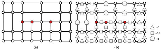
Figure 1.
Example of T-mesh: (a) example of T-mesh in index space; (b) configuration of knot intervals.
The expression of the T-spline surface is defined as
where is the control point for T-splines; is the T-spline basis function associated with ; is the weight for , as defined in the NURBS; and are the u-direction and v-direction B-spline basis functions of the control point . Each control point corresponds to a in the T-mesh. With the aforementioned definition of T-mesh in the index space, we can obtain the basis function associated with the control point.
The cubic T-mesh is widely discussed in the existing literature and is also studied in this work. Figure 2 shows an example of the basis function definition. The basis function associated with the control point is constructed from knot interval sequences inferred from its corresponding . The u-direction knot interval vector is obtained by traveling from the in positive and negative u-directions until (when , it is equal to 2) orthogonal are encountered, where represents the integer part of a real number. From Figure 2a,b, we can acquire the u-direction knot interval vector , where the value of is defined by knot intervals in Figure 1b. This is the same for the v-direction knot interval vector , as shown in Figure 2c. These two knot interval vectors define the rectangular support of the basis function associated to the control point (see the green area in Figure 2d). The B-spline basis functions and associated with the control point are defined by knot interval vectors and , respectively. The details of the B-spline basis function are presented in Appendix A.
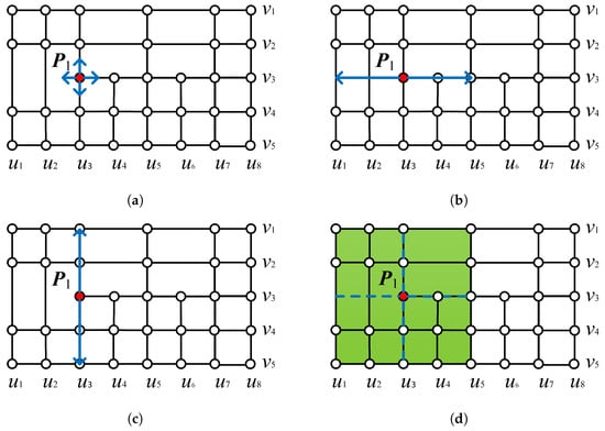
Figure 2.
The knot interval vectors corresponding to the control point : (a) traveling from the ; (b) u-direction knot interval vector; (c) v-direction knot interval vector; (d) domain of definition associated with the control point .
Figure 3 shows a structured bicubic T-spline surface and its corresponding T-mesh. Extraordinary points can further improve the topological flexibility of the T-mesh, and enable the representation of geometries with arbitrary topology using only one T-spline surface. The valence of a , denoted by , is the number of that emanate from that . Extraordinary points are either interior with that are not T-junctions or boundary with . The T-splines with extraordinary points are called unstructured T-splines. An unstructured bicubic T-spline surface is shown in Figure 4, where red circles represent extraordinary points.
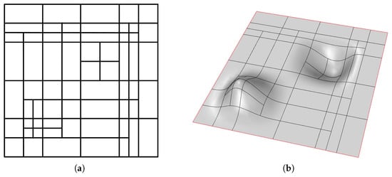
Figure 3.
Structured cubic T-mesh (a) and T-spline surfaces (b).
Figure 4.
Unstructured cubic T-mesh (a) and T-spline surfaces (b).
It is still a challenging problem when utilizing unstructured T-splines with extraordinary points in KL shell simulation because the C1 continuity requirement is difficult to achieve in the proximity of the extraordinary points. Recently, the D-patch method was employed to construct smooth spline functions around extraordinary points [43,49,50]. This method is also used in this research for investigating the elastoplastic analysis of more complex models.
2.2. BéZier Extraction
The Bézier extraction operator is used to convert T-spline elements into Bézier elements, and performs canonical treatment of T-junctions, which are similar to ‘hanging nodes’ and cannot be allowed in the mesh of the traditional finite element method. Figure 5a shows a cubic T-mesh, where the elements with red borders cannot achieve internal continuity due to the T-junctions (indicated by red circles). Through the segmentation of all the elements influenced by T-junctions, Bézier extraction delimits areas in which all element T-spline basis functions are . Therefore, these delimited polygons are called Bézier elements, as shown in Figure 5b. In addition, from the perspective of programming, the majority of classical finite element procedures, including parts of shell kinematics and nonlinear constitutive laws, could be easily reused in isogeometric analysis with the Bézier extraction method. To simplify the implementation of the visualization pipeline, only the Bézier mesh rather than T-mesh is plotted with the obtained results in this paper. The details of Bézier extraction are presented in [47,48].
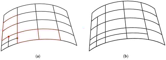
Figure 5.
The Bézier extraction of a T-mesh: (a) a cubic T-mesh; (b) Bézier mesh associated with the T-mesh in (a).
The mathematical basis of Bézier extraction is that over each element e of Bézier mesh, the localized B-spline basis function in Equation (1) can be expressed by coefficients and the same-degree Bernstein basis function , which is defined on the parameter field . The linear transformation over element e can be shown as
where p denotes the degree of the basis functions; for cubic T-spline surfaces, . In matrix-vector form, Equation (2) is written as
Thus, the blending function vector can be expressed as
where ; ; and the operator is defined as the dot product of vectors. The geometric map in the physical space can be expressed as
Naturally, we can acquire the displacement field:
where is the displacement vector of the control points for the element e. The computation of large deformation KL shells needs to evaluate the first and second derivatives of T-spline basis functions based on Bézier extraction. The derivatives of Equation (4) are presented in Appendix B.
3. Formulations for the Large Deformation of Elastoplastic Kirchhoff–Love Shells
In this section, we derive the finite strain plasticity model and the Kirchhoff–Love shell formulations, which will be used in the analysis. For more details, it is recommended to read references [51,52,53].
3.1. Finite Strain Plasticity
In our work, the rate-independent plasticity theory and the finite strain plastic model based on deformation gradient decomposition are employed as the theoretical foundations. The deformation gradient can be decomposed as the product of the elastic and plastic parts:
According to Equation (7), the plastic right Cauchy–Green deformation tensor is defined as
and the elastic left Cauchy–Green deformation tensor as
The elastic response is evaluated by the stored-energy function of the intermediate stress-free configuration, which can be decomposed into a volumetric and deviatoric part as
with
where and , and and are the bulk and the shear modulus.
The Cauchy stress can be calculated by the stored energy:
where is the second-order unit tensor; ; ; and and are the deviatoric and volumetric parts of the Kirchhoff stress . In order to compute the material yielding, there are two primary yield criteria. One is the maximum shear stress criterion, and the other is the von Mises yield criterion defined using multidimensional stress. It should be noted that the maximum shear yield surface is a polygon or a polyhedron, while the von Mises criterion yield surface is smooth. The smoothness of the yield surface makes it easy to find the yield point by numerical method. The classical von Mises yield function is computed from the deviatoric part of the Kirchhoff stress and the hardening function , written as
where is the hardening variable. The associative flow rule is used to describe material behavior during plastic deformation, which can be determined by the principle of maximum plastic dissipation. The rate form of the inverse of the plastic right Cauchy–Green deformation tensor can be expressed as
where and is the consistency parameter. The update of the hardening variable is governed by
The Kuhn–Tucker relationships are used to calculate the plastic consistency parameter under loading/unloading conditions:
With the preceding formulas, an algorithm for strain-driven return mapping is presented in Algorithm 1.
| Algorithm 1 Return mapping algorithm. |
| State: is computed in the time step , and are saved from the last time step |
| Input:, , |
| Output:, , |
|
In addition to the update of state variables as achieved by the return mapping algorithm in Algorithm 1, we also provide an algorithm to compute consistent elastoplastic material tangent , as listed in Algorithm 2. The tangent moduli can be obtained by taking the derivative of the Kirchhoff stress tensor with respect to the right Cauchy–Green deformation.
| Algorithm 2 Consistent elastoplastic tangent moduli. |
| Input: Same as Algorithm 1 |
| Output: |
|
3.2. Geometry Definition
Let be the curvilinear parametric coordinates of the midsurface and the through-thickness coordinate. In the following formulas, the Greek letters take the values , and the Latin letters take the values . The midsurface of the shell is represented by ; see Figure 6. In our work, the midsurface is described by the T-spline surface in Equation (5):
where is the control point and is the blending function. The tangent vector and the unit normal vector for any point in can be defined as
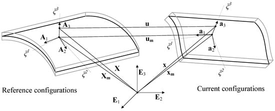
Figure 6.
Description of a KL shell for the different configurations.
The Kirchhoff–Love theory assumes that the cross-sectional fibers remain normal to the midsurface throughout the deformation. According to the KL shell theory, any point in the shell can be expressed by the midsurface and unit normal vector as
Calculating the partial derivative of the shell expression, we can acquire the covariant base vectors:
The metric coefficients are defined as
where the covariant metric coefficient and the covariant curvature coefficient are given as
Contravariant base vector can be computed as , where . It should be noted that in the above equations, we ignore the deformation in the thickness direction, which needs to be corrected in the next section.
3.3. Kinematics
The lowercase letters are used to indicate the deformed shell, and the uppercase letters indicate the undeformed shell. For the shell structures under finite strains, the right Cauchy–Green deformation tensor and the deformation gradient are represented as
The base vectors and are expressed in Equation (21), respectively defined in the deformed shell and the undeformed shell. Due to the fact that the deformation cannot be neglected in finite deformation, the thickness stretch is defined by , and the thickness base vector can be corrected as . Thus, Equation (24) can be modified by
is defined by the deformation of thickness, which cannot be directly computed from the deformation of the midsurface. Normally, the plane stress condition (the second Piola–Kirchhoff stress component ) is used to determine the unknown parameter :
In order to solve the plane stress constraint, an iterative calculation method is employed to update , as described in Algorithm 3.
The Green–Lagrange strain tensor is defined as . The plane Green–Lagrange strain components consist of membrane strain components and bending strain components :
where strains are computed by the covariant metric coefficients , and the covariant curvature coefficients , defined in Equation (23):
| Algorithm 3 Iterative update for . |
| Input:, |
| Output: |
|
The relationship between in-plane stresses and strains is given as
According to the plane stress constraint:
the material tensor is defined as
Membrane forces and bending moments are computed by integrating the second Piola–Kirchhoff stress tensor over the thickness:
Note that the three-dimensional material models described in Section 3.1 are defined in the local coordinate system. Therefore, a transformation between local Cartesian and curvilinear coordinates is necessary. A Cartesian coordinate associated with the shell midsurface is defined as follows:
is the base vector of local Cartesian coordinates with the upper bar standing for local nature. The deformation gradient for Cartesian coordinates can be given by
Similar transformations can be performed for the strain and the stress tensors.
3.4. Variational Formulation
The equilibrium equation is based on the principle of virtual work:
where and are the sum of internal and external work, respectively; and are the tensorial form of strain components defined in Equation (28); and and denote the initial integrating domain of the shell and the midsurface, with being the external load.
is the vector of external load. The internal nodal force vector can be obtained by the derivatives of with regards to nodal displacements . Its components are computed as
where is the r-th component of the nodal displacement vector. The components of the tangent stiffness matrix take the form of
Finally, the incremental displacement vector shall be solved via the linearized equation system:
3.5. Arc-Length Method
In the simulation of large deformation elastoplastic shells, overcritical behavior of the thin-walled structures, e.g., failure or buckling, and instabilities in the plastic material, similar to metals, will cause a nonlinear load–displacement equilibrium path, as shown in Figure 7. In such a case, a certain load may correspond to multiple displacement solutions, which makes the classical Newton–Raphson method in Section 3.4 invalid. For the computation of such an equilibrium path, the arc-length method [56,57,58] is a popular choice to apply a constraint equation , where is the load factor. The residual vector in (37) can be formulated as
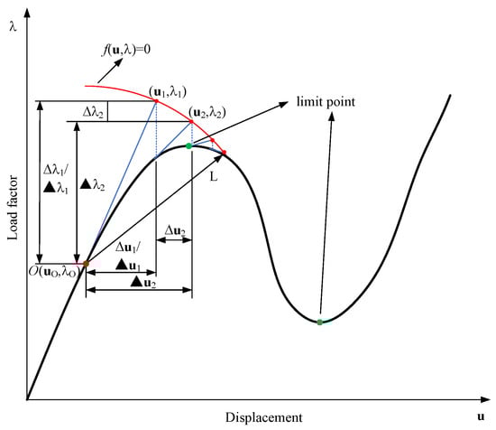
Figure 7.
Example of the arc-length method.
On the equilibrium path, . The incremental governing equations of the Newton–Raphson iterative method are based on a first-order Taylor series expansion about the equilibrium point with incremental displacement :
Equation (42) can be expressed as
where and . Hence, the displacement vector and load factor at the iterative step can be updated by
Equation (44) can be simplified by variable :
Let be the variable at the last convergence point O, as shown in Figure 7. Then, the variation of this variable at the iterative step can be defined as
Combing this with Equation (45), one gets
Herein, we use Crisfield’s arc-length method [57,58] to obtain . The constraint equation can be defined as
where L is the arc-length measure. Feeding Equation (47) into (48), one gets
For , with , , and , we acquire a predictor root
Because Equation (52) has two solutions, we need to confirm a better equilibrium path progression:
where and are computed from the last convergence step. In the subsequent iterative corrections, can be given by
The corrector root can be selected by
The complete algorithm of the arc-length method is summarized in Algorithm 4.
| Algorithm 4 The algorithm of arc-length method. |
| Input: The variables from the latest convergence point: |
| Output: The next convergence point, updated increments: |
|
4. Adaptive Refinement
In this section, we introduce the adaptive refinement method for isogeometric analysis of elastoplastic shells built with T-splines. The purpose of adaptive refinement is to improve analysis efficiency by refining the mesh locally. The classical ingredients of the adaptive method are 1. setup of a reliable error estimator; 2. generation of the new mesh according to the error estimator. A simple and accurate a posteriori error estimation was developed by Zienkiewicz and Zhu (the so-called ZZ estimate), employing post-processed stress fields to evaluate the error [59,60,61]. The ZZ estimate framework has been successfully applied to many fields of traditional finite element analysis, such as nonlinear analysis, dynamic problems, and fluid mechanics [62,63,64]. For isogeometric analysis, the a posteriori error estimator has also been applied to T-splines [65,66] and to hierarchical splines [67,68]. Subsequently, it has been extended to KL shells [69] and to trimmed models [70].
In our work, we employ the projection process to obtain the post-processed stress. is the stress result computed from the isogeometric analysis program. According to the assumption that the post-processed stress and the displacement are interpolated with the same function :
and
As explained in the reference [59], is a more accurate approximation than . Therefore, the error is estimated as
denotes the local error of the element “i”, which can be defined in the norm:
Another method to compute the local error in the so-called energy norm is introduced in the reference [71]. The global error can then be obtained by summing the local contributions of every element as
where “” represents the total number of elements.
The estimate of relative error is obtained as
Naturally, the refinement strategy depends on a predefined accuracy criterion. Thus, during the whole analysis process, the error needs to satisfy the condition
where is the prescribed error. If this condition is violated, the mesh is updated, and a recalculation for the current step is performed. We can judge which elements need to be refined by local error , and this local error is in fact computed in all elements. The local refinement parameter for each element is
The adaptive method will perform Quad-tree refinement on the elements of T-mesh, where the parameter , as shown in Figure 8.
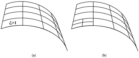
Figure 8.
The adaptive refinement based on the refinement parameter: (a) the initial T-mesh with the refinement parameter exceeding the threshold; (b) the T-mesh after adaptive refinement.
The linear independence of the T-mesh is an important consideration for applying the Galerkin method. Our proposed adaptive refinement method does not contain multiple knots since the T-mesh is obtained from Quad-tree refinement by inserting knots into the middle of adjacent ones. According to the reference [72] (Theorem 3. For a T-spline of degree and without multiple knots, its blending functions are linearly independent), our T-mesh applied for analysis is a subset of linear independent T-meshes.
5. Numerical Tests
In this section, five numerical tests are presented to illustrate the main advantages of applying T-spline-based isogeometric analysis to shell computations. Without losing generality, we use bicubic T-splines for analysis, and Gaussian points per computational element are used for midsurface integration, where p is the degree of the basis functions. Five Gaussian integration points in the thickness direction are used in all numerical examples. Firstly, three elastoplastic shell benchmarks are studied to verify the effectiveness of adaptive isogeometric methods using T-splines. Different relative errors are employed to control the process of adaptive refinement. The obtained results are compared with the reference results. Then, we compare the T-spline-based results with NURBS-based results. Finally, two shell models with cutouts are explored. We use unstructured T-splines, including extraordinary points, to represent shell models with the trimmed features and the D-patch framework to obtain the C1 continuity requirement.
5.1. Pinched Elastoplastic Hemisphere
The hemispherical shell is a standard benchmark problem in large elastoplastic deformation computations [34,36,73]. The geometry and boundary conditions are shown in Figure 9. Due to the symmetry of the hemisphere, one-quarter of this model can be used in the analysis process. Figure 9 also depicts the initial T-mesh of the computational model. The material parameters from the reference [36] are set as E = 100 N/mm and . The isotropic linear hardening law is used. The stress–strain relationship is shown in Figure 10, where we can see the strong nonlinearity of the elastoplastic material. The external force is loaded to 35 N and then unloaded to 0 N. The force–displacement responses of different prescribed error levels are plotted in Figure 11, where strong agreement with existing results [36] can be observed. The degrees of freedom (Dofs) throughout the adaptive analysis of loading processes and an example of the adaptive refinement step are given in Figure 12. In Figure 13, we show the displacement distribution of this model on the deformed configuration with the prescribed error .
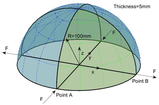
Figure 9.
Geometry and loading conditions of hemisphere.
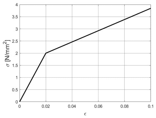
Figure 10.
The stress–strain relationship of the hemisphere.
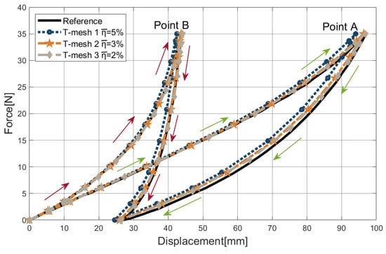
Figure 11.
The force–displacement responses of the pinched elastoplastic hemisphere.
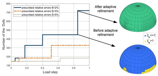
Figure 12.
The degrees of freedom throughout the adaptive analysis of the hemisphere.
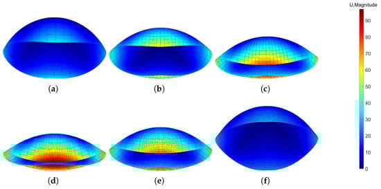
Figure 13.
The displacement magnitude of the pinched elastoplastic hemisphere (unit, mm): (a–d) loading stages with F = 10 N, 18 N, 26 N, 35 N; (e,f) unloading stages with F = 17 N, 0 N.
To demonstrate the greater computational efficiency of the adaptive method, we compare the relative error of adaptive refinement mesh with that of uniform refinement mesh. Due to the exact computation solution being unknown, the computation result of a uniform mesh (24,300 Dofs) is chosen as the reference solution . In addition, is the x-direction displacement of point A in the case of F = 35 N. The relative error is defined as . The error results of adaptive and uniform meshes are shown in Figure 14.
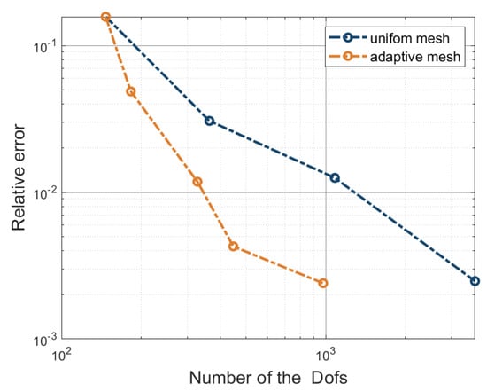
Figure 14.
The error plots of the hemisphere.
5.2. Pinched Elastoplastic Cylinder
This example considers a cylinder supported by two rigid diaphragms, pinched by two concentrated forces in opposite directions. This test is a typical and demanding benchmark example involving large plastic strains, out-of-plane warping, severe bending, and buckling through the loading process; see the references [34,35,36,74]. Figure 15 presents the initial geometry and boundary conditions. Exploiting symmetry, we apply only one octant of the cylinder to the simulation. The material parameters are chosen from the reference [34] as E = 3000 N/mm and , and the linear hardening law . The stress–strain relationship is shown in Figure 16. The arc-length control is employed in this example.The load–deflection curves of adaptive T-meshes with different prescribed error levels are shown in Figure 17. Our results are closely consistent with the solution from the reference [34]. In Figure 18, we present the Dofs of T-meshes during the adaptive computation process. The z-direction displacements at various loading stages with the prescribed relative error are reported in Figure 19, where we can see plastic buckling for large strains. From Figure 19, we can also observe that the mesh of the buckling region has been locally refined, which can provide a more reliable computational mesh for buckling analysis. In Figure 20, we present the number of iterations required in each increment to converge the response.
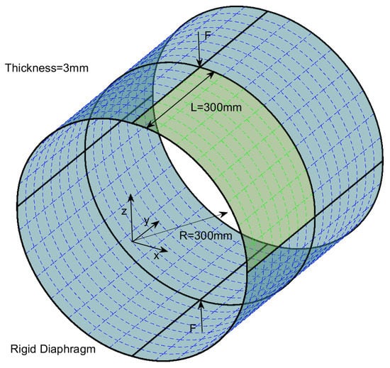
Figure 15.
Geometry and loading conditions of the cylinder.
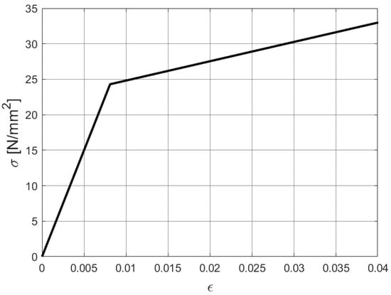
Figure 16.
The stress–strain relationship of the cylinder.
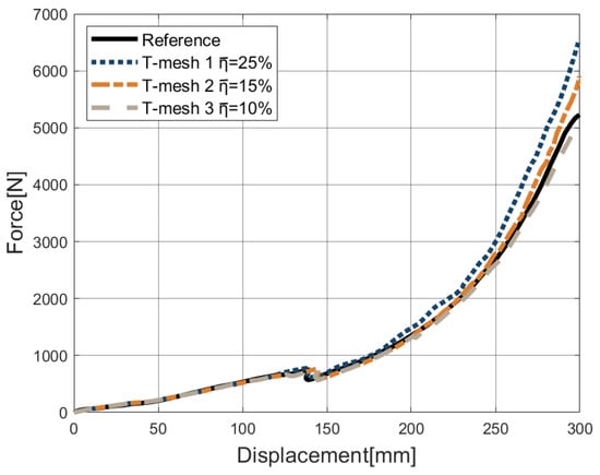
Figure 17.
Load–deflection curves of the pinched elastoplastic cylinder.
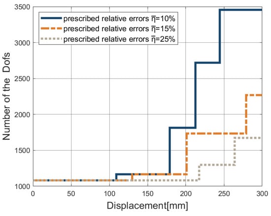
Figure 18.
The degrees of freedom throughout the adaptive analysis of the cylinder.
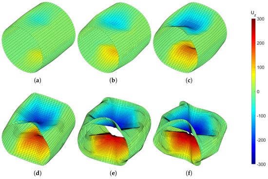
Figure 19.
The z-direction displacements of elastoplastic pinched cylinder: (a–f) the maximum values of the displacements are 51.52 mm, 104.40 mm, 150.96 mm, 201.72 mm, 249.90 mm, and 299 mm, respectively.
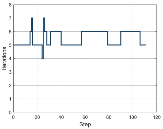
Figure 20.
The number of iterations in each increment.
In this example, we also compare the adaptive refinement with uniform refinement meshes by calculating the z-displacement of point A under F = 300 N. The computation result of a uniform mesh (24,300 Dofs) is chosen as the reference solution. Figure 21 depicts the comparison of the relative errors, which illustrates the better convergence of adaptive T-meshes.
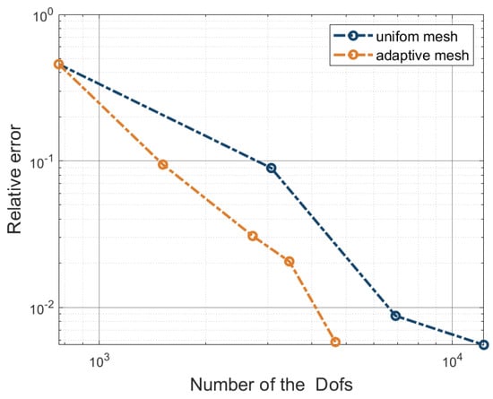
Figure 21.
The error plots of the cylinder.
5.3. Plastic Collapse of the Scordelis–Lo Roof
The collapse of the Scordelis–Lo roof under the action of gravity is investigated in this test, which is a classical benchmark for large deformation elastoplastic shell analysis; see the references [34,35,36,74]. The setup of the boundary conditions and initial geometry is presented in Figure 22. The material properties are E = 21,000 N/mm, , and perfect plasticity with taken from the reference [36]. The stress–strain relationship is shown in Figure 23, where we can see the feature of perfect plasticity.The roof is subjected to a uniform gravity-type load of = 0.004 N/mm and supported by rigid diaphragms at the ends. Due to the symmetry, only one-quarter of the roof is used for analysis. The arc-length control method is applied to this example. The load–deflection curve of point A obtained from the adaptive analysis is plotted in Figure 24, which agrees well with the solution from the reference [36]. The change in Dofs through the adaptive refinement with the prescribed relative error is shown in Figure 25. Figure 26 depicts the hardening variable () at different loading stages, where the plastic hinge at the top of the roof and elliptically shaped plastic hinges can be observed. These hinges are the salient characters of localized failure modes. We can also observe that the flexible topology of T-splines provides local refinement capabilities to increase mesh resolution where the plastic strains are large, e.g., around the plastic hinges.
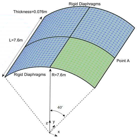
Figure 22.
Geometry and loading conditions of the Scordelis–Lo roof.
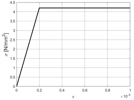
Figure 23.
The stress–strain relationship of the Scordelis–Lo roof.
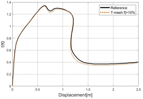
Figure 24.
The load–deflection curves of the point A on the Scordelis–Lo roof.
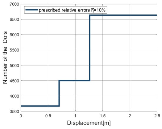
Figure 25.
The degrees of freedom throughout the adaptive analysis of the Scordelis–Lo roof.
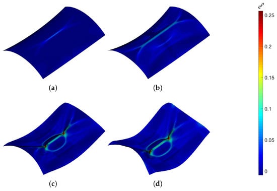
Figure 26.
Collapse of the Scordelis–Lo roof; hardening variables distribution for different deformation stages: (a–d) the z-direction displacements of point A = 0.51223, 1.0129, 1.5082, and 2.5 m, respectively.
The comparison of the convergence between adaptive refinement and uniform mesh is also performed in this example. The z-direction displacement of point A with computed by a uniform mesh with 19,200 Dofs is regarded as the reference solution. The greater efficiency of the adaptive refinement can be observed in Figure 27.
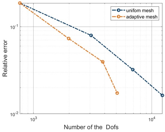
Figure 27.
The error plots of the Scordelis–Lo roof.
5.4. Plastic Cylinder with Holes Under Compression
Next, a pinched cylinder with trimmed features is analyzed. The cylindrical sheet with cutouts is a common structure in engineering. The geometry and boundary conditions are depicted in Figure 28. Only one octant of the cylinder is used. From Figure 28, we can observe that the T-splines can represent a model with cutouts by a single patch, which can be directly applied to isogeometric analysis without reparameterization. The material properties are E = 800 N/mm, , and the hardening function . The stress–strain relationship is shown in Figure 29. The value of the load is set as F = 2.35 N. The prescribed relative error of this example is set as 10%. Our resulting load–displacement curve is compared with the reference solution obtained from ABAQUS (14381 S4R shell elements) [75], as shown in Figure 30, where we can see a good agreement. In Figure 31, the displacement fields of IGA and FEA (ABAQUS) are compared. We can also observe that the adaptive refinement is applied around the point load. The accuracy of the trimmed model analysis in our work is confirmed by these results.
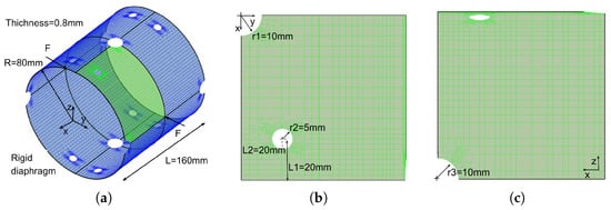
Figure 28.
(a–c) The geometry and boundary conditions of the trimmed cylinder.
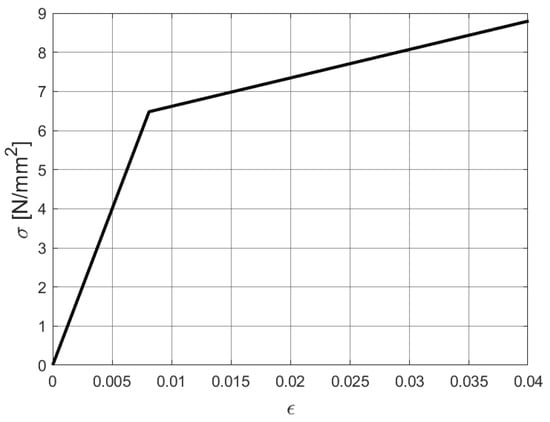
Figure 29.
The stress–strain relationship of the trimmed cylinder.
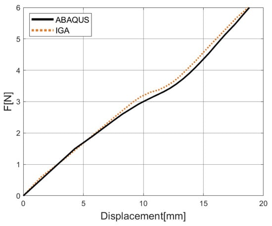
Figure 30.
Load–displacement curves of the trimmed cylinder.
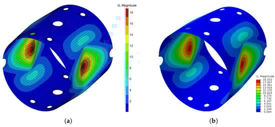
Figure 31.
The displacement magnitude of the trimmed cylinder: (a) result of IGA; (b) result of FEA.
5.5. Torsion of a Plastic Rectangular Sheet with a Hole
In the last example, the torsion of a rectangular sheet with a hole is analyzed. The geometry and boundary conditions are set up in Figure 32. The material properties are E = 210 N/m, , and isotropic linear hardening with . The stress–strain relationship is shown in Figure 33. In this test, the prescribed relative error of this example is . The rotation boundary condition () is applied to the right side of the model. Because the x-displacement of the right side is fixed, the change in the x-displacement reaction force with the rotation is shown in Figure 34, where a good agreement with ABAQUS results can be observed. In Figure 35, we can see that our results are closely consistent with those computed from ABAQUS (15047 S4R shell elements) [75]. In this example, the adaptive refinement region is near the clamped side. This example involves the finite rotation, the large plastic strains, and the model with the trimmed features, which can represent the applicability of our work in these aspects.
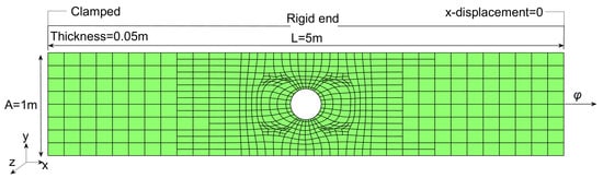
Figure 32.
The geometry and boundary conditions of the plastic rectangular shell with a hole.
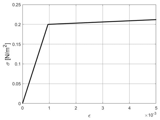
Figure 33.
The stress–strain relationship of the rectangular shell.
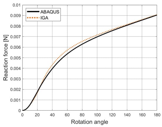
Figure 34.
The moment–angle curves of the rectangular shell with a hole.
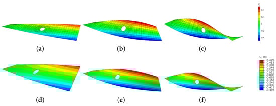
Figure 35.
The z-displacement of the rectangular shell at various deformation stages: (a–c) result from IGA, rotation angle 60°, 120°, 180°; (d–f) result from FEA, rotation angle 60°, 120°, 180°.
6. Conclusions
We have extended the isogeometric Kirchhoff–Love shell computational model based on T-splines to large deformation elastoplastic problems, with the advantages of representing the trimmed model with one single patch and local refinement capability. The proposed formulation is able to deal with large elastoplastic strains as well as finite rotations, which is validated by various benchmarks. The results are compared with those from references and FEA (ABAQUS), confirming the accuracy and efficiency of the method we implemented.
In our paper, five Gaussian integration points are used in the thickness direction, which is a time-consuming calculation process. Simo and Kennedy [73] advocated an approach based on directly expressing moment versus curvature relations for elastoplastic shells. What is more, Armen et al. [76] proposed a novel implicit rate type response relation, bypassing the integration of elastoplastic stress–strain relationships across the thickness of the beam at each time step. These methods may bring efficiency and accuracy to the isogeometric analysis of elastoplastic Kirchhoff–Love shells, and will be considered in our future study.
In our current adaptive analysis framework, if the relative error is greater than the prescribed error, the local refinement will be performed. Similarly, if the relative error is less than another specified value, a mesh recovery should be performed, which can reduce the number of equations to be solved and improve computational efficiency. The refinement of T-mesh is based on the knot insertion algorithm of the B-spline curve so that the geometry can remain unchanged. However, in the process of mesh recovery, geometric errors will be caused by knot removal. Multiresolution techniques and a suitable geometric error tolerance should be taken into account. The mesh recovery of T-splines for adaptive analysis will be a challenging topic in future research.
Author Contributions
Conceptualization, M.G., G.Z. and W.W.; methodology, X.D. and M.G.; software, M.G.; validation, M.G., R.Z. and J.Y.; formal analysis, M.G.; investigation, M.G., R.Z. and J.Y.; resources, G.Z. and W.W.; data curation, M.G.; writing—original draft preparation, M.G.; writing—review and editing, W.W. and X.D.; visualization, X.D. and M.G.; supervision, G.Z.; project administration, G.Z.; funding acquisition, G.Z. All authors have read and agreed to the published version of the manuscript.
Funding
The work is supported by National Natural Science Foundation of China (Project Nos. 61972011, 62102012, 62002004, and 52175213) and the Project is funded by China Postdoctoral Science Foundation (Project No. 2021M690294).
Institutional Review Board Statement
Not applicable.
Informed Consent Statement
Not applicable.
Data Availability Statement
Not applicable.
Conflicts of Interest
The authors declare no conflict of interest.
Appendix A
Assume that represents the knot vector of the p-degree B-spline basis function, where ui is the ith knot value, and n is equal to the number of control points minus 1. It is worth noting that when the B-spline basis function corresponds to a T-spline control point, n is equal to 0. The B-spline basis may be defined using a recurrence relation, starting with the piecewise constant () basis function:
For , the B-spline basis function is defined using the Cox–de Boor recursion formula:
For the T-splines, since one control point only corresponds to one basis function, let :
References
- Hughes, T.J.; Liu, W.K. Nonlinear finite element analysis of shells: Part I. Three-dimensional shells. Comput. Methods Appl. Mech. Eng. 1981, 26, 331–362. [Google Scholar] [CrossRef]
- Hughes, T.J.; Liu, W.K. Nonlinear finite element analysis of shells-part II. two-dimensional shells. Comput. Methods Appl. Mech. Eng. 1981, 27, 167–181. [Google Scholar] [CrossRef]
- Li, Z.X.; Wei, H.; Vu-Quoc, L.; Izzuddin, B.A.; Zhuo, X.; Li, T.Z. A co-rotational triangular finite element for large deformation analysis of smooth, folded and multi-shells. Acta Mech. 2021, 232, 1515–1542. [Google Scholar] [CrossRef]
- Rezaiee-Pajand, M.; Arabi, E.; Masoodi, A.R. A triangular shell element for geometrically nonlinear analysis. Acta Mech. 2018, 229, 323–342. [Google Scholar] [CrossRef]
- Li, Z.; Li, T.; Vu-Quoc, L.; Izzuddin, B.; Zhuo, X.; Fang, Q. A nine-node corotational curved quadrilateral shell element for smooth, folded, and multishell structures. Int. J. Numer. Methods Eng. 2018, 116, 570–600. [Google Scholar] [CrossRef]
- Rezaiee-Pajand, M.; Masoodi, A.R. Shell instability analysis by using mixed interpolation. J. Braz. Soc. Mech. Sci. Eng. 2019, 41, 419. [Google Scholar] [CrossRef]
- Rezaiee-Pajand, M.; Masoodi, A.R.; Arabi, E. A 6-parameter triangular flat shell element for nonlinear analysis. Eur. J. Comput. Mech. 2019, 28, 237–268. [Google Scholar] [CrossRef]
- Cottrell, J.A.; Hughes, T.J.; Bazilevs, Y. Isogeometric Analysis: Toward Integration of CAD and FEA; John Wiley & Sons: Hoboken, NJ, USA, 2009. [Google Scholar]
- Hughes, T.J.; Cottrell, J.A.; Bazilevs, Y. Isogeometric analysis: CAD, finite elements, NURBS, exact geometry and mesh refinement. Comput. Methods Appl. Mech. Eng. 2005, 194, 4135–4195. [Google Scholar] [CrossRef]
- Cottrell, J.A.; Reali, A.; Bazilevs, Y.; Hughes, T.J. Isogeometric analysis of structural vibrations. Comput. Methods Appl. Mech. Eng. 2006, 195, 5257–5296. [Google Scholar] [CrossRef]
- Cottrell, J.; Hughes, T.; Reali, A. Studies of refinement and continuity in isogeometric structural analysis. Comput. Methods Appl. Mech. Eng. 2007, 196, 4160–4183. [Google Scholar] [CrossRef]
- Bouclier, R.; Elguedj, T.; Combescure, A. Efficient isogeometric NURBS-based solid-shell elements: Mixed formulation and B-method. Comput. Methods Appl. Mech. Eng. 2013, 267, 86–110. [Google Scholar] [CrossRef]
- Bouclier, R.; Elguedj, T.; Combescure, A. On the development of NURBS-based isogeometric solid shell elements: 2D problems and preliminary extension to 3D. Comput. Mech. 2013, 52, 1085–1112. [Google Scholar] [CrossRef]
- Oesterle, B.; Sachse, R.; Ramm, E.; Bischoff, M. Hierarchic isogeometric large rotation shell elements including linearized transverse shear parametrization. Comput. Methods Appl. Mech. Eng. 2017, 321, 383–405. [Google Scholar] [CrossRef]
- Echter, R.; Oesterle, B.; Bischoff, M. A hierarchic family of isogeometric shell finite elements. Comput. Methods Appl. Mech. Eng. 2013, 254, 170–180. [Google Scholar] [CrossRef]
- Benson, D.; Bazilevs, Y.; Hsu, M.C.; Hughes, T. Isogeometric shell analysis: The Reissner-Mindlin shell. Comput. Methods Appl. Mech. Eng. 2010, 199, 276–289. [Google Scholar] [CrossRef]
- Dornisch, W.; Klinkel, S.; Simeon, B. Isogeometric Reissner–Mindlin shell analysis with exactly calculated director vectors. Comput. Methods Appl. Mech. Eng. 2013, 253, 491–504. [Google Scholar] [CrossRef]
- Dornisch, W.; Klinkel, S. Treatment of Reissner–Mindlin shells with kinks without the need for drilling rotation stabilization in an isogeometric framework. Comput. Methods Appl. Mech. Eng. 2014, 276, 35–66. [Google Scholar] [CrossRef]
- Dornisch, W.; Müller, R.; Klinkel, S. An efficient and robust rotational formulation for isogeometric Reissner–Mindlin shell elements. Comput. Methods Appl. Mech. Eng. 2016, 303, 1–34. [Google Scholar] [CrossRef]
- Du, X.; Zhao, G.; Wang, W. Nitsche method for isogeometric analysis of Reissner-Mindlin plate with non-conforming multi-patches. Comput. Aided Geom. Des. 2015, 35, 121–136. [Google Scholar] [CrossRef]
- Zhao, G.; Du, X.; Wang, W.; Liu, B.; Fang, H. Application of isogeometric method to free vibration of Reissner-Mindlin plates with non-conforming multi-patch. Comput. Aided Des. 2017, 82, 127–139. [Google Scholar] [CrossRef]
- Kiendl, J.; Bletzinger, K.U.; Linhard, J.; Wüchner, R. Isogeometric shell analysis with Kirchhoff–Love elements. Comput. Methods Appl. Mech. Eng. 2009, 198, 3902–3914. [Google Scholar] [CrossRef]
- Kiendl, J.; Hsu, M.C.; Wu, M.C.; Reali, A. Isogeometric Kirchhoff–Love shell formulations for general hyperelastic materials. Comput. Methods Appl. Mech. Eng. 2015, 291, 280–303. [Google Scholar] [CrossRef]
- Kiendl, J. Isogeometric Analysis and Shape Optimal Design of Shell Structures. Ph.D. Thesis, Technische Universität München, Munich, Germany, 2011. [Google Scholar]
- Nguyen-Thanh, N.; Kiendl, J.; Nguyen-Xuan, H.; Wüchner, R.; Bletzinger, K.U.; Bazilevs, Y.; Rabczuk, T. Rotation free isogeometric thin shell analysis using PHT-splines. Comput. Methods Appl. Mech. Eng. 2011, 200, 3410–3424. [Google Scholar] [CrossRef]
- Benson, D.J.; Bazilevs, Y.; Hsu, M.C.; Hughes, T. A large deformation, rotation-free, isogeometric shell. Comput. Methods Appl. Mech. Eng. 2011, 200, 1367–1378. [Google Scholar] [CrossRef]
- Duong, T.X.; Roohbakhshan, F.; Sauer, R.A. A new rotation-free isogeometric thin shell formulation and a corresponding continuity constraint for patch boundaries. Comput. Methods Appl. Mech. Eng. 2017, 316, 43–83. [Google Scholar] [CrossRef]
- Benson, D.; Hartmann, S.; Bazilevs, Y.; Hsu, M.C.; Hughes, T. Blended isogeometric shells. Comput. Methods Appl. Mech. Eng. 2013, 255, 133–146. [Google Scholar] [CrossRef]
- Lai, W.; Yu, T.; Bui, T.Q.; Wang, Z.; Curiel-Sosa, J.L.; Das, R.; Hirose, S. 3-D elasto-plastic large deformations: IGA simulation by Bézier extraction of NURBS. Adv. Eng. Softw. 2017, 108, 68–82. [Google Scholar] [CrossRef]
- Yu, T.; Lai, W.; Bui, T.Q. Three-dimensional elastoplastic solids simulation by an effective IGA based on Bézier extraction of NURBS. Int. J. Mech. Mater. Des. 2019, 15, 175–197. [Google Scholar] [CrossRef]
- Elguedj, T.; Hughes, T.J. Isogeometric analysis of nearly incompressible large strain plasticity. Comput. Methods Appl. Mech. Eng. 2014, 268, 388–416. [Google Scholar] [CrossRef]
- Elguedj, T.; Bazilevs, Y.; Calo, V.M.; Hughes, T.J. B and F projection methods for nearly incompressible linear and non-linear elasticity and plasticity using higher-order NURBS elements. Comput. Methods Appl. Mech. Eng. 2008, 197, 2732–2762. [Google Scholar] [CrossRef]
- Taylor, R. Isogeometric analysis of nearly incompressible solids. Int. J. Numer. Methods Eng. 2011, 87, 273–288. [Google Scholar] [CrossRef]
- Ambati, M.; Kiendl, J.; De Lorenzis, L. Isogeometric Kirchhoff–Love shell formulation for elasto-plasticity. Comput. Methods Appl. Mech. Eng. 2018, 340, 320–339. [Google Scholar] [CrossRef]
- Huynh, G.; Zhuang, X.; Bui, H.; Meschke, G.; Nguyen-Xuan, H. Elasto-plastic large deformation analysis of multi-patch thin shells by isogeometric approach. Finite Elem. Anal. Des. 2020, 173, 103389. [Google Scholar] [CrossRef]
- Alaydin, M.D.; Benson, D.J.; Bazilevs, Y. An updated Lagrangian framework for Isogeometric Kirchhoff–Love thin-shell analysis. Comput. Methods Appl. Mech. Eng. 2021, 384, 113977. [Google Scholar] [CrossRef]
- Perić, D.; Vaz, M., Jr.; Owen, D. On adaptive strategies for large deformations of elasto-plastic solids at finite strains: Computational issues and industrial applications. Comput. Methods Appl. Mech. Eng. 1999, 176, 279–312. [Google Scholar] [CrossRef]
- Han, C.S.; Wriggers, P. An h-adaptive method for elasto-plastic shell problems. Comput. Methods Appl. Mech. Eng. 2000, 189, 651–671. [Google Scholar] [CrossRef]
- Hu, Y.; Randolph, M. H-adaptive FE analysis of elasto-plastic non-homogeneous soil with large deformation. Comput. Geotech. 1998, 23, 61–83. [Google Scholar] [CrossRef]
- Sederberg, T.W.; Zheng, J.; Bakenov, A.; Nasri, A. T-splines and T-NURCCs. ACM Trans. Graph. 2003, 22, 477–484. [Google Scholar] [CrossRef]
- Sederberg, T.W.; Cardon, D.L.; Finnigan, G.T.; North, N.S.; Zheng, J.; Lyche, T. T-spline simplification and local refinement. ACM Trans. Graph. (TOG) 2004, 23, 276–283. [Google Scholar] [CrossRef]
- Bazilevs, Y.; Calo, V.M.; Cottrell, J.A.; Evans, J.A.; Hughes, T.J.R.; Lipton, S.; Scott, M.A.; Sederberg, T.W. Isogeometric analysis using T-splines. Comput. Methods Appl. Mech. Eng. 2010, 199, 229–263. [Google Scholar] [CrossRef]
- Casquero, H.; Wei, X.; Toshniwal, D.; Li, A.; Hughes, T.J.; Kiendl, J.; Zhang, Y.J. Seamless integration of design and Kirchhoff–Love shell analysis using analysis-suitable unstructured T-splines. Comput. Methods Appl. Mech. Eng. 2020, 360, 112765. [Google Scholar] [CrossRef]
- Scott, M.A.; Simpson, R.N.; Evans, J.A.; Lipton, S.; Bordas, S.P.; Hughes, T.J.; Sederberg, T.W. Isogeometric boundary element analysis using unstructured T-splines. Comput. Methods Appl. Mech. Eng. 2013, 254, 197–221. [Google Scholar] [CrossRef]
- Casquero, H.; Liu, L.; Zhang, Y.; Reali, A.; Kiendl, J.; Gomez, H. Arbitrary-degree T-splines for isogeometric analysis of fully nonlinear Kirchhoff–Love shells. Comput. Aided Des. 2017, 82, 140–153. [Google Scholar] [CrossRef]
- Liu, N.; Hsu, M.C.; Lua, J.; Phan, N. A large deformation isogeometric continuum shell formulation incorporating finite strain elastoplasticity. Comput. Mech. 2022, 70, 965–976. [Google Scholar] [CrossRef]
- Scott, M.A.; Borden, M.J.; Verhoosel, C.V.; Sederberg, T.W.; Hughes, T.J.R. Isogeometric finite element data structures based on Bézier extraction of T-splines. Int. J. Numer. Methods Eng. 2011, 88, 126–156. [Google Scholar] [CrossRef]
- Borden, M.J.; Scott, M.A.; Evans, J.A.; Hughes, T.J. Isogeometric finite element data structures based on Bézier extraction of NURBS. Int. J. Numer. Methods Eng. 2011, 87, 15–47. [Google Scholar] [CrossRef]
- Reif, U. A refineable space of smooth spline surfaces of arbitrary topological genus. J. Approx. Theory 1997, 90, 174–199. [Google Scholar] [CrossRef]
- Toshniwal, D.; Speleers, H.; Hughes, T.J. Smooth cubic spline spaces on unstructured quadrilateral meshes with particular emphasis on extraordinary points: Geometric design and isogeometric analysis considerations. Comput. Methods Appl. Mech. Eng. 2017, 327, 411–458. [Google Scholar] [CrossRef]
- Simo, J.C.; Hughes, T.J. Computational Inelasticity; Springer: Berlin/Heidelberg, Germany, 2006; Volume 7. [Google Scholar]
- Simo, J.C. A framework for finite strain elastoplasticity based on maximum plastic dissipation and the multiplicative decomposition: Part I. Continuum formulation. Comput. Methods Appl. Mech. Eng. 1988, 66, 199–219. [Google Scholar] [CrossRef]
- Simo, J.C. A framework for finite strain elastoplasticity based on maximum plastic dissipation and the multiplicative decomposition. Part II: Computational aspects. Comput. Methods Appl. Mech. Eng. 1988, 68, 1–31. [Google Scholar] [CrossRef]
- Du, X.; Zhao, G.; Wang, W.; Guo, M.; Zhang, R.; Yang, J. NLIGA: A MATLAB framework for nonlinear isogeometric analysis. Comput. Aided Geom. Des. 2020, 80, 101869. [Google Scholar] [CrossRef]
- Kim, N.H. Introduction to Nonlinear Finite Element Analysis; Springer Science & Business Media: Berlin/Heidelberg, Germany, 2014. [Google Scholar]
- Wriggers, P. Nonlinear Finite Element Methods; Springer Science & Business Media: Berlin/Heidelberg, Germany, 2008. [Google Scholar]
- Ritto-Corrêa, M.; Camotim, D. On the arc-length and other quadratic control methods: Established, less known and new implementation procedures. Comput. Struct. 2008, 86, 1353–1368. [Google Scholar] [CrossRef]
- Crisfield, M.A. A fast incremental/iterative solution procedure that handles “snap-through”. In Proceedings of the Symposium on Computational Methods in Nonlinear Structural and Solid Mechanics, Washington, DC, USA, 6–8 October 1981; pp. 55–62. [Google Scholar] [CrossRef]
- Zienkiewicz, O.C.; Zhu, J.Z. A simple error estimator and adaptive procedure for practical engineerng analysis. Int. J. Numer. Methods Eng. 1987, 24, 337–357. [Google Scholar] [CrossRef]
- Zienkiewicz, O.C.; Zhu, J.Z. The superconvergent patch recovery and a posteriori error estimates. Part 1: The recovery technique. Int. J. Numer. Methods Eng. 1992, 33, 1331–1364. [Google Scholar] [CrossRef]
- Zienkiewicz, O.C.; Zhu, J.Z. The superconvergent patch recovery and a posteriori error estimates. Part 2: Error estimates and adaptivity. Int. J. Numer. Methods Eng. 1992, 33, 1365–1382. [Google Scholar] [CrossRef]
- Wiberg, N.E.; Zeng, L.; Li, X. Error estimation and adaptivity in elastodynamics. Comput. Methods Appl. Mech. Eng. 1992, 101, 369–395. [Google Scholar] [CrossRef]
- Zeng, L.F.; Wiberg, N.E. Spatial mesh adaptation in semidiscrete finite element analysis of linear elastodynamic problems. Comput. Mech. 1992, 9, 315–332. [Google Scholar] [CrossRef]
- Zienkiewicz, O.; Liu, Y.; Huang, G. Error estimation and adaptivity in flow formulation for forming problems. Int. J. Numer. Methods Eng. 1988, 25, 23–42. [Google Scholar] [CrossRef]
- Dörfel, M.R.; Jüttler, B.; Simeon, B. Adaptive isogeometric analysis by local h-refinement with T-splines. Comput. Methods Appl. Mech. Eng. 2010, 199, 264–275. [Google Scholar] [CrossRef]
- Guo, M.; Zhao, G.; Wang, W.; Du, X.; Yang, J. T-Splines for Isogeometric Analysis of Two-Dimensional Nonlinear Problems. Comput. Model. Eng. Sci. 2020, 123, 821–843. [Google Scholar] [CrossRef]
- Vuong, A.V.; Giannelli, C.; Jüttler, B.; Simeon, B. A hierarchical approach to adaptive local refinement in isogeometric analysis. Comput. Methods Appl. Mech. Eng. 2011, 200, 3554–3567. [Google Scholar] [CrossRef]
- Wang, P.; Xu, J.; Deng, J.; Chen, F. Adaptive isogeometric analysis using rational PHT-splines. Comput. Aided Des. 2011, 43, 1438–1448. [Google Scholar] [CrossRef]
- Antolin, P.; Buffa, A.; Coradello, L. A hierarchical approach to the a posteriori error estimation of isogeometric Kirchhoff plates and Kirchhoff–Love shells. Comput. Methods Appl. Mech. Eng. 2020, 363, 112919. [Google Scholar] [CrossRef]
- Coradello, L.; Antolin, P.; Vázquez, R.; Buffa, A. Adaptive isogeometric analysis on two-dimensional trimmed domains based on a hierarchical approach. Comput. Methods Appl. Mech. Eng. 2020, 364, 112925. [Google Scholar] [CrossRef]
- Yunus, S.; Pawlak, T.; Wheeler, M. Application of the Zienkiewicz-Zhu error estimator for plate and shell analysis. Int. J. Numer. Methods Eng. 1990, 29, 1281–1298. [Google Scholar] [CrossRef]
- Wang, A.; Zhao, G.; Li, Y.D. Linear independence of the blending functions of T-splines without multiple knots. Expert Syst. Appl. 2014, 41, 3634–3639. [Google Scholar] [CrossRef]
- Simo, J.C.; Kennedy, J. On a stress resultant geometrically exact shell model. Part V. Nonlinear plasticity: Formulation and integration algorithms. Comput. Methods Appl. Mech. Eng. 1992, 96, 133–171. [Google Scholar] [CrossRef]
- Başar, Y.; Itskov, M. Constitutive model and finite element formulation for large strain elasto-plastic analysis of shells. Comput. Mech. 1999, 23, 466–481. [Google Scholar] [CrossRef]
- Abaqus, G. Abaqus 6.11; Dassault Systemes Simulia Corporation: Providence, RI, USA, 2011. [Google Scholar]
- Wang, Z.; Srinivasa, A.R.; Rajagopal, K.; Reddy, J. Simulation of inextensible elasto-plastic beams based on an implicit rate type model. Int. J. Non-Linear Mech. 2018, 99, 165–172. [Google Scholar] [CrossRef]
Disclaimer/Publisher’s Note: The statements, opinions and data contained in all publications are solely those of the individual author(s) and contributor(s) and not of MDPI and/or the editor(s). MDPI and/or the editor(s) disclaim responsibility for any injury to people or property resulting from any ideas, methods, instructions or products referred to in the content. |
© 2023 by the authors. Licensee MDPI, Basel, Switzerland. This article is an open access article distributed under the terms and conditions of the Creative Commons Attribution (CC BY) license (https://creativecommons.org/licenses/by/4.0/).