Abstract
Laminated glass composed of several layers of glass plies bonded to a polymer interlayer enjoys ever growing interest in modern architecture. Being often used in impact protection designs requires understanding of both pre- and post-breakage behavior of these structures. This paper contributes to this subject by examining an application of an explicit phase field dynamic model to the description of fracture in a laminated glass subjected to a low velocity impact. The achieved results indicate the ability of the proposed model to successfully describe the onset of damage and subsequent crack propagation. It has, however, been observed that a relatively fine mesh is needed to interpolate a sharp discontinuity accurately, which makes this approach computationally demanding. The model is first validated against experimental results obtained for a single-layer float glass. Next, the usability of the phase-field damage model as a crack predictor in individual layers of the composite is investigated. The dependence of the results on residual stiffness, element type, and initial tensile strength is examined and discussed.
1. Introduction
Owing to its high aesthetic value, laminated glass enjoys an ever growing interest in modern architecture. It typically consists of several layers of glass and polymeric viscous interlayers [1]. This constitution retains the functional properties of an ordinary glass, but its properties after cracking are improved [2] as interlayers hold individual fragments of fractured glass together, thus partially preventing a catastrophic failure. Although experimental work plays a key role in promoting new structures to practical applications, an effective structure can hardly be designed without numerical simulations addressing the response of a given structure to a variety of conditions not generally accessible experimentally.
Developing a robust and accurate computational model for glass laminates is a complex task. While layered configuration may prevent collapse and improves post breakage behavior, its simulation proves complicated as glass is essentially damaged by brittle failure with a very small process zone and negligible ductility. Although a number of numerical techniques applied to float or laminated glass have been proposed, this scientific topic is still widely open to further investigation. See, for example, [3] for an extensive overview of numerical methods applied to float glass, where the standard finite element method with the Rankine failure criterion is compared to the extended finite element method, discrete element method, and their combinations. Similarly, some critical aspects and several modeling techniques applied to laminated glass structures are presented in [4,5]. The application of peridynamic models [6] is also worth mentioning.
At present, a very promising approach to the modeling of brittle fracture is the application of the phase-field model [7,8]. The principal advantage of this family of models is its ability to predict crack initialization as well as crack branching [9] with no additional ad hoc criteria. This is attributed to variational consistency as the crack development arises directly from the energy minimization of the regularized functional for a brittle material.
The present paper examines the ability of the phase field model to simulate gradual fracture of a laminated glass subjected to several consecutive low velocity impacts. This issue has already been investigated in [10] with the help of commercial LS-DYNA software where the results of an extensive experimental program were also presented. Attention is therefore afforded to theoretical and computational aspects of the phase field model in light of plates [11], while experimental measurements used to support our numerical implementation are outlined only briefly just for the sake of completeness. Proceeding in the footsteps of [10], the five (5LG) and seven (7LG) layer laminates consisting of three and four plies of a float glass bonded to a PVB (polyvinyl butyral) interlayers are examined, respectively. In particular, the ability of the phase field model to estimate the response of a laminated glass observed experimentally is tested by comparing the measured and simulated distributions of contact force and gradually evolving crack patterns.
The remainder of the paper is structured as follows. We begin with a short review of the experimental part of the project in Section 2. Essential details of the spatially reduced Mindlin Reissner model with phase field damage are introduced in Section 3. Remarks on time integration and implementation of the Hertz contact and interlayer viscoelasticity are also presented. Numerical implementation including the modeling strategy is discussed first in Section 4 in the framework of a single glass ply (SG) followed by the simulation of the two selected laminates in Section 5. A thorough discussion arising from a comparative study with experimental measurements is also provided. The principal outcomes are finally summarized in Section 6.
2. Experiments
The concept of sacrificial-glass-ply design [12] was adopted in [10] to propose two specific geometries. In such a case, the outer glass layers are made thinner as they mainly serve to protect the inner glass layers, which in turn play the key role in accommodating the applied load. Additionally, the outer glass layers are expected to crack to dissipate, together with the polymer interlayers, the impactor energy thus enhancing the bearing capacity of the laminated structure. Herein, the 5LG laminate is composed of three glass layers and two PVB interlayers, whereas the 7LG laminate consists of four glass layers bonded to three PVB interlayers. An illustrative example of such a laminate is displayed in Figure 1. Geometrical details of both composites are stored in Table 1.
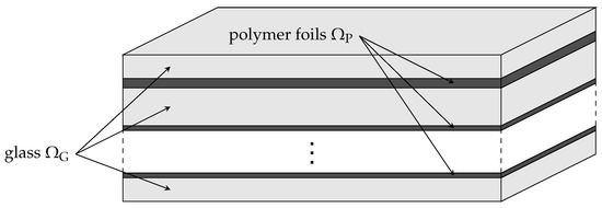
Figure 1.
Example of a laminated glass.

Table 1.
Geometry of 5-layer (5LG) and 7-layer (7LG) laminated glass samples.
The tested samples were suspended in a vertical position on a pair of steel ropes along vertical edges to approximate free boundary conditions [13], thus eliminating the effect of mechanical supports. The low velocity impact was induced horizontally via an 800 mm long pendulum device (impactor) having a cylindrical shape with a hemispherical nose with the diameter of 50 mm. The required impact energy, defined as the kinetic energy of the impactor with the impact velocity , was achieved by dropping the 48.2 kg impactor from a given height . To examine the influence of subsequent impacts of growing intensity on a laminate fracture response, the impact height was gradually increased by 5 cm as seen in Table 2.
Table 2.
Overview of fractured glass layers after individual impacts including impact energies. With the left-hand side impacted, the symbols |•| indicate the previously fractured glass layers, empty spaces | | the unfractured ones, and circles |∘| the crack initiation in a glass layer.
For illustration, we present the results of three particular samples of the two laminates. The response of individual samples after individual impacts is summarized in Table 2. Considering the impacted glass on the left-hand side, the empty circle |∘| indicates the onset of damage in a given ply, whereas the filled circle |•| identifies a glass layer which has already been broken during previous impacts. Empty spaces | | represent unbroken glass layers.
Although limited to three samples only, the results confirm the advantage of a sacrificial-glass-ply design which expects the outer glass layers to fracture, so the inner glass layers are still capable of sustaining further loads. This is particularly evident for samples where the impacted glass layer fractured at the initial stage of loading (5LG-1, 7LG-1, 7LG-3). Unfortunately, the results also suggest a certain degree of variability in fracture response of laminates potentially attributed to a random distribution of initial surface flaws of unprotected (outer) glass layers. This was also confirmed by our study on a single glass ply in [14] devoted merely to the application of various damage models implemented in the LS-DYNA software. These findings make the predictive capability of any numerical model rather difficult especially in the framework of deterministic modeling. To perform stochastic simulations goes, however, beyond the present scope owing mainly to insufficient experimental data to identify, for example, a statistical distribution of impact energies. Instead, we concentrate on tuning the computational model to represent one particular experiment. If successful, this will serve as a stepping stone for more complex stochastic analysis.
The final crack patterns are presented in Figure 2 and Figure 3 showing a typical distribution of radial cracks of different lengths seldomly connected by short parts of secondary cracks. In addition, notice that, apart from diagonal cracks, the cracks bend to arrive at the sample edges in a perpendicular direction. This is discussed when comparing the fracture patterns with numerical predictions.

Figure 2.
Final fracture patterns of 5LG samples.
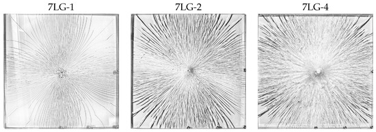
Figure 3.
Final fracture patterns of 7LG samples.
3. Phase-Field Model
The application of phase field model to damage has afforded considerable attention; see [8,15,16] (to cite a few), so only the basic relations are reviewed in this section focusing on the formulation in the context of layered plate theory, time integration, aspects of implementation of the Hertz contact, and the issue of viscoelasticity.
The model is based on variational framework of a brittle fracture [17], where the bulk energy competes with the dissipated energy via energy minimization. To this end, the Hamilton’s principle of stationary action is employed and the displacement field and crack topology are obtained by minimizing the action integral
where is the time from a given range. Minimizing this functional may prove unfeasible as it is performed over all admissible crack topologies . To remedy this, the phase-field model brings regularization and introduces a scalar damage field d, which represents a relative measure of damage as a transition from the intact material to a fully damaged material indicating a crack. Therefore, the action integral is dependent on two continuous fields u and d instead of a discontinuous topological set , i.e.,
which is more suitable for finite element implementation. The kernel of this integral is called the Lagrangian and, for a linear dynamic system, it reads
where , , , are the kinetic energy, the elastic energy, the dissipated energy, and the external work, respectively. We assume that the first and the last terms are not affected by the phase field model. Thus, assuming an elastic domain with the density loaded by external tractions over provides
The remaining two terms, i.e., the elastic potential , representing the stored energy of an undamaged material, and dissipated energy then allow for the transition from a purely elastic response to the phase-field damage model. The present formulation complies with the physical requirement permitting the compressive stress to be transmitted across the crack even for a fully damaged material with . Hence, the elastic energy is decomposed into an active (tensile) part , which is degraded by the damage field, and a passive (compressive) part , which remains independent of the damage field, to obtain
where the strain energy densities are defined later in Section 3.4.
The last term in the Lagrangian (3) is the regularized dissipated energy given by
where and l are the material parameters, and function controls the type of regularization. Moreover, the constant is fully determined by function as ; see [15] for detailed description of individual terms. A specific format of function is elaborated later in Section 3.4 providing details of the assumed decomposition.
3.1. Time Discretization
Standard finite difference method is used to integrate Equation (2) in time which gives the discrete form of the action integral for time instances in the form
The adopted discrete form of the Lagrangian leads to the explicit central difference scheme for fields , , where represents the time step assumed constant in the present study. This is particularly advantageous as minimization of Equation (7) can be performed for the displacement field u and the damage parameter d separately.
These equations are identical to purely elastic response except for the elastic energy being divided into an active and a passive part. Note that this decomposition is performed on the displacement field at time instant , while the unknown displacement field at time is determined explicitly. The only difficulty of this scheme is thus the decomposition of strain energy density .
Minimizing the discrete format of action integral (7) () with respect to the phase-field damage parameter d yields
In order to arrive at a physically correct crack evolution and no crack healing, the pointwise irreversibility condition must be additionally imposed
Regardless of the choice of function , the irreversibility condition (13) makes the weak form (12) a nonlinear problem that needs to be solved as a variational inequality.
For the sake of clarity, the presented explicit dynamic procedure [18] is schematically represented in Figure 4. Finally, note that the spatial distribution of fields u and d is found in a standard way using the finite element method.
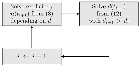
Figure 4.
Flowchart of the central difference phase-field algorithm.
3.2. Mindlin Plate Model
A full 3D model is computationally demanding which suggests that application of a more effective spatially reduced plate model. We start from a single layer model which will be subsequently extended to laminated plates. The Mindlin–Reissner theory, which assumes that the cross-section remains planar after deformation but not necessarily perpendicular to the midsurface of the plate, is adopted. Commonly, the model is obtained by assuming a linear distribution of displacements and rotations and subsequent through-thickness integration. Owing to damage, this integration must be carried out numerically. The elastic energy then receives the form
where the overall thickness h is numerically divided into individual layers i of thickness with in-plane stress and strain vectors, see Figure 5. The midsurface with the coordinate system is the new spatially reduced domain of interest. Point out that the parameter is an auxiliary material constant which indicates that the amount of shear subjected to damage, i.e., whether the shear stress is still transmitted across the crack. Notice that only the part of out-of-plane shear contribution that enters the active part of strain energy density is degraded by function .
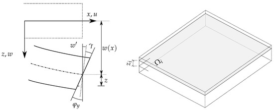
Figure 5.
Graphical representation of Mindlin plate theory.
The constitutive equations for in-plane stress and strain fields and out-of-plane shear stresses and strains are provided by
where represents the plane stress stiffness tensor expressed in terms of Lame’s coefficients and and is the identity tensor.
The strains and follow from standard strain–displacement relations and are written in terms of in-plane displacements , out of plate deflection w, and rotations of the cross section as
where the matrix is given by
Equation (12) is also subjected to spatial reduction via through-thickness integration to obtain
where the integrated active part of the strain energy density
drives the damage evolution. In this regard, it appears useful to replace the strain energy density by a constant representing the strain energy density calculated on the basis of the maximum tensile stress. This rewrites Equation (21) as
3.3. Layered Mindlin Plate Model
Consider a plate consisting of N layers indexed by , recall Figure 1. The indices are therefore reserved for the glass layers. Several options are available to enforce displacement continuity at common interfaces. In some applications, the use of Lagrangian multipliers proves advantageous as these are directly linked to the interface shear stresses. However, grounding the formulation of the present model on explicit dynamics calls for the reduction of the number of degrees of freedom as much as possible. Therefore, the continuity of in-plane displacement u is enforced directly by substitution considering the following two kinematic constraints:
The first equation enforces the out-of-plane incompressibility of the layers and the latter one represents the in-plane displacement continuity at the interfaces. The formulation for glass layers, identified by odd indices , remains intact, whereas kinematic variables of damage-free interlayers with even indices are substituted by expressions determined by restrictions (24) and (25) as
As an illustrative example, consider a 5-layer laminate (three solid glasses and two interlayers) which, after substitution, is fully described by seven unknowns: .
It should also be mentioned that the layered plate model requires solving Equation (23) for each glass layer. This allows for different crack patterns to develop in individual layers.
3.4. Model Selection and Decomposition
The phase field model is determined by the decomposition of strain energy density into active and passive parts and by the selection of function .
The most physically sound response is simulated using spectral decomposition of functional (5) proposed in [19]. However, this decomposition contains singularities in the finite element application and resulted in instabilities in our simulations. On the hand, stable solutions were experienced when considering the decomposition based on a volumetric-deviatoric split as suggested in [20]. The active and passive contributions to the strain energy density are then given by
where is a deviatoric part of the strain tensor , and K is the bulk modulus.
As for the dissipation function, the model is valid for an arbitrary choice of . The present formulation follows Pham [21] and considers a simple relation
with the degradation function defined as
Unlike common representation of a dissipation function suggested by Bourdin et al. [17], which considers damage evolution already at the onset of loading, the adopted linear version allows for postponing the damage initiation beyond this point, and so not affecting the initial transfer of energy from the impactor into the plate.
For the present choice of , the fracture energy can be written in terms of the tensile strength , Young’s modulus E, and the length scale parameter l as [22]
While strictly valid for one-dimensional (1D) setting, Equation (33) is generally adopted also for simulations in higher dimensions. Owing to the presence of length scale parameter l, typically equal to two times the characteristic length of the smallest element in the finite element mesh [19]; this relation is also mesh dependent.
For a typical edge length of a triangular element of 2 mm employed for the analysis of laminates discussed in Section 2, the fracture energy stored in Table 3 may considerably exceed a typical value of Jm used for glass. While the value of MPa corresponds to the characteristic quasi-static strength in tensile bending defined by the European Standard EN 16612 [23], the larger values, e.g., MPa, used particularly in the analysis of a single glass ply, represents the initial value of tensile strength we adopted to postpone the onset of damage in numerical simulations and consequently to arrive at the glass response comparable with experimental observations. Point out that even larger values of the initial tensile strength were considered in [10]. Since at the onset of damage this value almost immediately drops down to the actual strength of 45 MPa, the associated fracture energy enters the analysis only at a very beginning stage of fracture process; see Section 4 ahead for further details. Nevertheless, realistic values of would still call for much smaller elements to avoid snap-back at a material level. On the contrary, this would lead to computationally unfeasible simulations. Thus, only the large values around 300 Jm to simulate the crack propagation were tested in all present calculations.
Table 3.
Fracture energies of glass for quasi-static bending and initial tensile strength and given length scale parameter l.
3.5. Hertz Contact
The transfer of kinetic energy from the impactor to the glass plate is implemented through a simple Hertz relation. The contact force is then given by
where is the displacement of the impactor, is the out of plane displacement of the impacted node with the coordinate . The positive part operator ensures that the contact force is transmitted during the impactor penetration only. The proportionality constant k (contact stiffness) is written as
where R is the radius of the impactor and and are the Young modulus and Poisson ratio of the glass plate and impactor, respectively. Although the force is nonlinear, it can be introduced into the variational framework using pseudopotential
The impactor represents an additional degree of freedom so its contribution
must be supplemented to the overall kinetic energy.
3.6. Viscoelasticity of Interface Layer
The response of a polymer interlayer is significantly time-dependent. However, even in a low velocity impact, the response time is in the range of milliseconds, so that the rate dependency can be neglected and an empirical rule can be used to evaluate its current shear stiffness. In particular, adopting the rule [24], the instantaneous shear modulus of the interlayer is provided by
where is the current time and is the actual temperature. Function can be approximated by the Generalized Maxwell chain model [25] as
where N stands for the number of Maxwell units. The corresponding shear stiffnesses associated with the selected relaxation times are obtained by fitting Equation (39) to experimental measurements [26,27]. The temperature shift factor follows from the well known Williams–Landel–Ferry equation
In the present study, we adopt the results derived for the PVB interlayer in [26]. These are summarized in Table 4 complemented with kPa. The constants and were found for the reference temperature T0 = 20 °C.
Table 4.
Parameters of generalized Maxwell chain model representing PVB foil for reference temperature T0 = 20 °C.
4. Damage of Single Glass Ply
The explicit dynamic model is first validated for a single glass ply focusing on both the state before and after the crack initiation. A nondestructive step allows us to check the ability of the computational model and the Hertz contact to predict the dynamic response of glass, whereas the damage step identified the capability of the phase field model. To this end, both the evolution of contact force and displacements at points recorded experimentally were monitored to gain information on how the energy is transferred from the impactor into the glass laminate. While the experiment is described in detail in [14], the presented experimental results have not been published yet.
With reference to tested samples, a glass plate with dimensions 0.5 m × 0.5 m, recall also Table 1, is examined. Because of symmetry, only a quarter of the model with appropriate symmetry boundary conditions is considered. The material parameters of both the glass and impactor needed in numerical simulations are summarized in Table 5. As already mentioned in Section 2, the radius R of the impactor head entering Equation (35) is set to 50 mm.
Table 5.
Material parameters of float glass and steel impactor.
An example of the finite element mesh made of triangular elements is presented in Figure 6. To support the use of these elements in numerical analysis of laminates, the application of bilinear quadrilateral plate elements with reduced integration of out-of-plane shear is also tested and compared with a full three-dimensional (3D) calculations exploiting higher order tetrahedral elements. Details of the adopted finite element meshes are listed in Table 6.
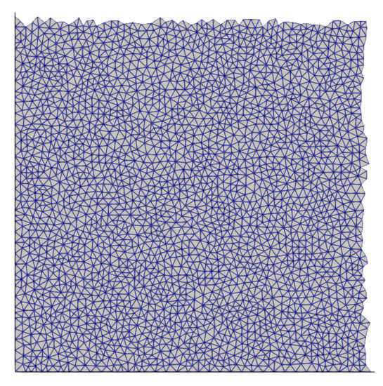
Figure 6.
Example of finite element mesh consisting of a random grid of 3-node triangular elements.
Table 6.
Details on finite element mesh.
The impact of element type and the corresponding mesh on the ply response is tested first considering a simple example of a plate weakened by an initial crack. The plate is impacted with the energy of 148 J (impact height of 30 cm). The initial crack is introduced by enforcing the damage for coordinates to spread over the width of two elements (Figure 7 left) for a given value of the shear parameter ; recall Equations (14) and (15). In accordance with Section 3.4, we set , where is the edge length of the smallest element in the mesh.
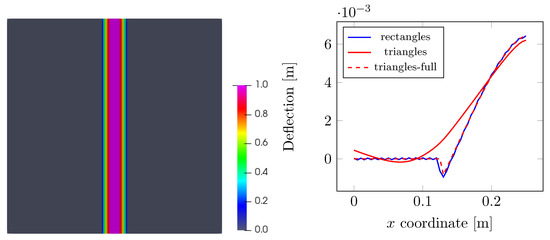
Figure 7.
Initial damage distribution on quarter plate (left) and deflection distribution along the x-axis for triangular and quadrilateral elements and for triangular elements with assumed shear damage with () denoted as triangles-full (right).
The variation of deflection across the crack at the selected time s is plotted in Figure 7 on the right side. The solid lines represent the case of no damage in shear with ; thus, only the bending part in Equation (15) is affected by damage and the shear strains contribute entirely to . While the mesh with quadrilateral elements provides reasonable response, we see that, for a triangular mesh, the wave passes across the crack. This can be attributed to spurious shear strain transfer. However, when degrading the the whole out-of-plane shear contribution by setting (the shear contribution now taken entirely by is fully degraded by function ) in the analysis with a triangular mesh, we arrive at the expected response as shown by the dashed line.
The next example addresses a non-destructive test allowing us to compare the experimentally measured contact force with numerical predictions up to the impact height of 30 cm. The results for various types of meshes, recall Table 6, are presented in Figure 8a for cm. As seen, all meshes provide a comparable response matching well the experimental measurements. However, it has been observed that four node quadrilateral elements, albeit using one point integration in shear, experience a zero energy mode manifested by local vibration from element to element. For that reason and given the results in Figure 7, the triangular mesh in Figure 6 with shear degradation option was used in all subsequent analyses. Its applicability is further promoted by the comparative study displayed in Figure 8b, where a reasonable agreement with experimental results is suggested even for a relatively high impact energy.
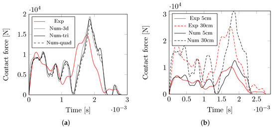
Figure 8.
Comparison of evolution of measured and predicted contact force for nondestructive test: (a) influence of finite element type—impact height of 10 cm; (b) application of triangular mesh for impact heights of 5 cm and 30 cm.
The last experiment is concerned with adjusting the onset of damage. This is because the stress calculated in the contact zone between an impactor and glass exceeds the glass strength earlier than the glass breaks in experiments [13,28]. This is quite important also with the phase-field analysis. For illustration, we consider a destructive test where the tested sample broke already at the impact height cm. The results appear in Figure 9, Figure 10 and Figure 11.
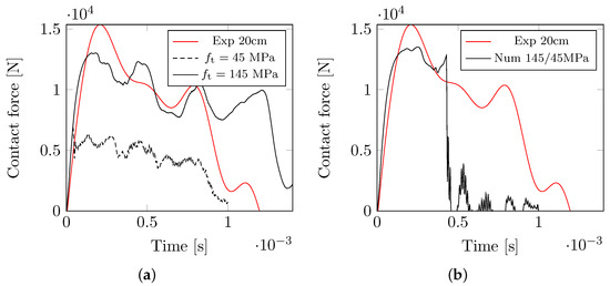
Figure 9.
Comparison of evolution of measured and predicted contact force for destructive test: (a) constant tensile strength; (b) variable tensile strength.
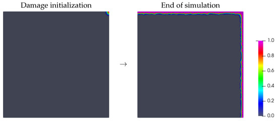
Figure 10.
Damage evolution for single glass ply with static tensile strength.
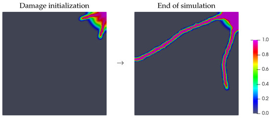
Figure 11.
Damage evolution for single glass ply with adjusted initial tensile strength.
Figure 9a indicates that assuming the actual static tensile strength MPa promotes the damage initiation too early in comparison to the experimental results, while delaying the onset of damage via artificially increasing the tensile strength to MPa shows a considerable improvement in the prediction of the contact force. Figure 10 further suggests that controlling the crack initiation by MPa does not generate sufficient energy to drive a rapid crack evolution and crack branching as observed experimentally [10,14].
A remedy is provided by restoring the initial high tensile strength to its physically correct value at the onset of damage [10], i.e., MPa. The former value ensures accommodation of sufficient energy, whereas the latter value allows its rapid dissipation leading to more realistic crack pattern. While seemingly simple, this step still deserves attention, particularly in the framework of the presented phase field model.
Remind that the evolution of damage is driven by fracture energy. However, the relationship between the tensile strength and fracture energy provided by Equation (33) is valid for 1D analysis only. When used with a general 3D analysis, such calculated fracture energy may lead to damage initiation for stresses, which do not exceed the prescribed tensile strength. Thus, in the present study, the point of switching the analysis from initial state controlled by the initial value of fracture energy to the one associated with the actual tensile strength of MPa, recall Table 3, is determined by reaching the value of the damage parameter in the most stressed element. This can be mathematically represented as
From that point on, the subsequent fracturing process in an arbitrary element continues with the value of associated with MPa and the mesh dependent length scale parameter l set to mm in all simulations involving the triangular mesh.
This approach resulted in the damage pattern seen in Figure 11 with the corresponding evolution of the contact force depicted in Figure 9b. Note that the shear reduction parameter was set to a threshold value of to avoid through thickness penetration of the impactor. The accumulation of energy by using increased initial tensile strength allows for formation of more random crack patterns. With a sufficiently large difference between the actual and initial tensile strengths, the model promotes cracks in multiple directions. On the other hand, we see a notable mismatch in the descending part of the measured and predicted contact force, Figure 9b. This can be attributed to the fact that the impactor gradually penetrates into the already broken fragments. Similar results, derived with the help of LS-DYNA software, have been observed in [14] both in terms of crack pattern and contact force evolution.
5. Damage of Laminated Glass Plate
The results presented in the previous section now open the door to the simulation of laminates exploiting the theoretical framework outlined in Section 3.3.
Similar to the experimental program discussed in Section 2, we address both types of laminates with their geometrical details provided in Table 1. The material properties of the impactor and glass layers are taken from Table 5. For the polymer interlayer, we set the density kg/m. The Poisson ratio 0.49 is considered to approach a volumetrically incompressible material while avoiding a significant shear locking. Given the room temperature during experiments in the range of 24.9 °C to 26 °C, we set in Equation (40) to 25 °C. As suggested in Section 3.6, the viscoelastic properties of the interlayer are included only empirically via Equation (38). No other material parameters of the PVB interlayer are needed as damage is expected to occur in the glass layers only.
To validate implementation of the layered plate theory, we begin again with nondestructive tests. For the sake of brevity, attention is limited to 5LG-3 and 7LG-2 samples as these show a similar evolution of gradual damage due to repeating impacts of variable intensity; see Table 2. The response of both types of laminates is examined through the distribution of contact force for two impact heights causing no damage. The results plotted in Figure 12 indicate a satisfactory agreement between numerical predictions and experimental measurements, thus excluding any systematic error potentially linked to numerical implementation. The observed differences are merely associated with the 8th-pole Butterworth low-pass filter (2× CFC 1000 filter) we used to filter out the frequencies associated with vibrations of the impactor from the measured accelerations [10]. Apart from eliminating the initial data before the largest amplitudes (approximately 0.3–0.4 ms of a signal) and the final part (after 20 ms) with small oscillations affected significantly by the experimental noise, the filter was applied to the entire time domain associated with experimental measurements. The eliminated data could have affected the initial slope of the experimentally observed contact force so its direct comparison with numerical predictions might be misleading.
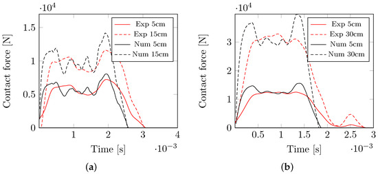
Figure 12.
Comparison of evolution of measured and predicted contact force for nondestructive test: (a) 5LG-3 laminate; (b) 7LG-2 laminate.
Moving to damage brings to mind the key role of the initial tensile strength we suggested in the previous section. Its value influences the amount of energy available in the glass to drive the fracture process. This is illustrated in Figure 13 assuming two different values of the initial tensile strength . Similarly to the result presented in Figure 11, the strength was reduced to MPa according to Equation (41). The damage patterns at the onset of cracking and at the time when the damage fully localized into isolated cracks are shown for the back glass layer (the furthermost from the impacted one) of a 5LG-laminate loaded by the impact energy of 236 J (impact height of 50 cm). It is evident that the value of the initial tensile strength qualitatively changes the result of the simulation. One may therefore consider this value as another material parameter albeit depending on a given computational model. For MPa, the damage initiated at ms, whereas, for MPa, it was delayed to ms. While the time to stabilize the crack growth was in both cases about the same, the larger amount of energy dissipated in the latter case resulted in a significantly denser crack pattern. It follows that choosing the value of sensitively the model is able to control the branching and development of multiple cracks with no additional ad hoc criteria.
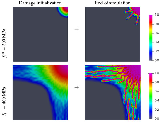
Figure 13.
Damage evolution in back glass layer of 5LG laminate for two values of initial tensile strength .
As the solution depends on the length scale parameter l, which in turn is estimated from the underlying finite element mesh, it appears useful to briefly address this issue. Proceeding with the previously studied 5LG laminate, we keep the initial tensile strength MPa and assume the impact energy of 236 J (impact height of 50 cm). The first example compares structured and unstructured meshes sketched in Figure 14 (bottom figures). Considering a comparable mesh density, the length of the process zone is set to mm for all tested meshes. The damage patterns for the time instant ms are compared in Figure 14 (top figures) for two examples of structured meshes and one example of the unstructured mesh; recall Figure 6. The evolution of damage along preferential direction associated with the structured meshes is evident.

Figure 14.
Damage distribution for three different meshes.
The second example addresses the effect of mesh refinement considering two mesh densities, a coarser mesh with 9425 elements and the process zone mm (left) and a finer mesh with 19,119 elements and the process zone mm (right) being essentially the one in Figure 6. It has been found that the mesh density influences the onset of damage, i.e., the transition point . The damage initiation is delayed with increasing the element size with the time at the onset of damage ms and ms for the coarser and finer mesh, respectively. The damage patterns plotted in Figure 15 correspond to time ms. While the onset of damage and partially also the crack pattern differ, the crack growth velocity appears similar for both meshes. A potential reason for decreasing the initiation time with increasing the mesh refinement can be attributed to the reduction of the fracture process zone leading to a brittle failure when approaching this parameter to zero. This issue is under current investigation.
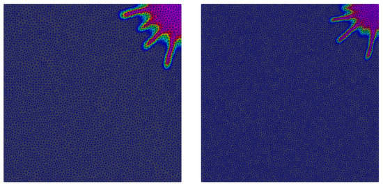
Figure 15.
Impact of mesh density on damage initiation () and subsequent evolution ( ms): coarser mesh left ( ms), finer mesh right ( ms).
The above findings are finally exploited in the simulation of gradual damage caused by several consecutive impacts for the selected laminates. The finer element mesh in Figure 15, recall also Figure 6, was used providing a satisfactory agreement between the measured and predicted contact force. Point out that, with repeating impacts, the new calculation always started from the damage state associated with the previous loading step. We begin with the 5LG-3 sample. To correctly predict the onset of damage for a given impact height cm, the initial tensile strength MPa was used. The distribution of the contact forces is presented in Figure 16a.
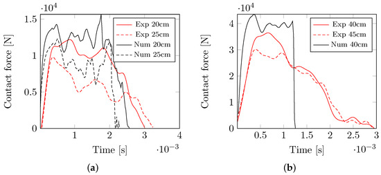
Figure 16.
Comparison of evolution of measured and predicted contact force for destructive test: (a) 5LG-3 laminate; (b) 7LG-2 laminate.
In agreement with experiment, the back layer fractured first. To force the damage to progress to another layer required increasing the impact height to 25 cm. Similarly to experiments, the layers cracked gradually from the back layer towards the impacted one. Unlike experiments, however, both remaining layers cracked at this simulation step. The evolution of damage in individual layers is displayed in Figure 17 for the selected time instances. It is worth mentioning that the same value of was prescribed to all layers, whereas, in [10], each layer was assigned a different value of to follow the experimentally observed cracking sequence as close as possible. Since this was not the principal objective of this study, primarily focusing on the potential of phase field to model fracture in laminated glass, we did not investigate this issue any further.
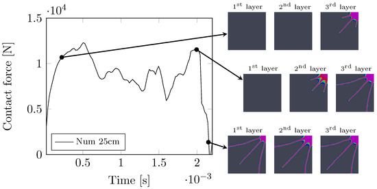
Figure 17.
Evolution of cracks in 5LG laminate due to impact height cm; the 1st layer is the impacted one.
Similar conclusions can be drawn from the simulations of the 7LG laminate as only the onset of damage was meant to be captured in agreement with the experiment performed on 7LG-2 sample. To this end, the value of was considered. As the same value was again assigned to all layers, it is not surprising, pointing out a relatively large impact energy that all layers fractured within this single simulation step. This is also why only one numerically generated contact force is presented in Figure 16b. The corresponding evolution of cracks at selected simulation times is available in Figure 18.
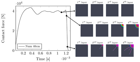
Figure 18.
Evolution of cracks in 7LG laminate due to impact height cm, the 1st layer is the impacted one.
To arrive at better agreement with experiment, both in terms of the contact force variation and fracture sequence, would require more gentle tuning of the initial tensile strength on the one hand and assigning a different value of this parameter to individual layers on the other hand. The latter option would cause the contact force to decay more gradually [10]. However, as already mentioned, this goes beyond the present scope.
6. Conclusions
The paper described application of the phase-field model to the modeling of gradual evolution of damage in laminated glass structures subjected to low-velocity impact of increasing intensity. To reduce computational complexity, the theory was introduced in the framework of the layered Mindlin plate theory with piecewise constant distribution of out-of-plane shear stresses. Further simplifications included the transfer of kinetic energy from the impactor into the glass layer through the liner Hertz law (36), calculation of the instantaneous shear modulus via the rule (38), and the use of relation (33) in 3D simulations, albeit strictly valid for 1D setting only. Such formulated model allowed us to perform all calculations very efficiently with the help of a fully explicit dynamic solver. The principal observations are:
- Introducing a properly selected initial tensile strength to accommodate sufficient energy prior to the onset of cracking appears crucial to correctly track the evolution of damage, thus supporting our observations presented in [10]. This was demonstrated by comparing the distribution of the contact force and gradually evolving crack pattern with the experimental results. The phase field model then proved its ability to predict the expected sequence of fracture of individual glass layers as well as crack branching within these layers. Owing to a random behavior of glass laminates, partially associated with random nature of initial flaws in the glass, this parameter, hardly deterministic, reduces the predictive capability of any damage model applied to the modeling of impact resistance of such structures. To promote the current approach in predictive or parametric studies, the simulations should be potentially presented in the stochastic framework once data from a sufficiently broad experimental program are available.
- Given the presence of the length scale parameter to provide regularization, these models are mesh dependent both in terms of the element size and mesh orientation. However, because the leading Equation (23) follows from the minimization of total energy, the convergence of the solution can be expected upon a sufficient mesh refinement. In this regard, an unstructured mesh made of 3-node triangular elements with degraded contribution of out-of-plane shear was found to be optimal.
- Unlike the predicted density of cracks, the crack orientation and path, turning towards the plate edges, is fully compatible with experimental observations. To arrive at improved prediction of the crack pattern might require more accurate, physically sound, contact rule. The linear model based on the Hertz law is too localized and cannot accurately describe the contact between the glass fragments and the impactor head and thus to ensure proper transition of the kinetic energy into the plate.
Author Contributions
Conceptualization: J.S., T.J. and M.Š.; Methodology: J.S. and T.J.; Experimental work: M.Š.; Numerical implementation: J.S. and T.J.; Writing—original draft: J.S.; Writing—review and editing: M.Š.; Supervision: T.J.; Project administration: M.Š. All authors have read and agreed to the published version of the manuscript.
Funding
We are thankful for financial support provided by the Czech Science Foundation, project No. 22-15553S.
Institutional Review Board Statement
Not applicable.
Data Availability Statement
All computer codes implemented in open source FEniCS are publicly available in gitlab repository [29].
Conflicts of Interest
The authors declare no conflict of interest.
References
- Haldimann, M.; Luible, A.; Overend, M. Structural Use of Glass; Structural Engineering Documents; IABSE: Zürich, Switzerland, 2008; Volume 10. [Google Scholar]
- Zhao, C.; Yang, J.; Wang, X.e.; Azim, I. Experimental investigation into the post-breakage performance of pre-cracked laminated glass plates. Constr. Build. Mater. 2019, 224, 996–1006. [Google Scholar] [CrossRef]
- Wang, X.E.; Yang, J.; Liu, Q.F.; Zhang, Y.M.; Zhao, C. A comparative study of numerical modelling techniques for the fracture of brittle materials with specific reference to glass. Eng. Struct. 2017, 152, 493–505. [Google Scholar] [CrossRef]
- Chen, S.; Zang, M.; Wang, D.; Yoshimura, S.; Yamada, T. Numerical analysis of impact failure of automotive laminated glass: A review. Compos. Part B Eng. 2017, 122, 47–60. [Google Scholar] [CrossRef]
- Teotia, M.; Soni, R. Applications of finite element modelling in failure analysis of laminated glass composites: A review. Eng. Fail. Anal. 2018, 94, 412–437. [Google Scholar] [CrossRef]
- Ma, Q.; Wu, L.; Huang, D. An extended peridynamic model for dynamic fracture of laminated glass considering interfacial debonding. Compos. Struct. 2022, 290, 115552. [Google Scholar] [CrossRef]
- Hofacker, M.; Miehe, C. Continuum phase field modeling of dynamic fracture: Variational principles and staggered FE implementation. Int. J. Fract. 2012, 178, 113–129. [Google Scholar] [CrossRef]
- Pham, K.; Ravi-Chandar, K.; Landis, C. Experimental validation of a phase-field model for fracture. Int. J. Fract. 2017, 205, 83–101. [Google Scholar] [CrossRef]
- Bourdin, B.; Larsen, C.J.; Richardson, C.L. A time-discrete model for dynamic fracture based on crack regularization. Int. J. Fract. 2011, 168, 133–143. [Google Scholar] [CrossRef]
- ZemanovÁ, A.; Hála, P.; Konrád, P.; Sovjak, R.; Šejnoha, M. Gradual Fracture of Layers in Laminated Glass Plates under Low-Velocity Impact. Comput. Struct. 2022. under review. [Google Scholar]
- Kikis, G.; Ambati, M.; De Lorenzis, L.; Klinkel, S. Phase-field model of brittle fracture in Reissner–Mindlin plates and shells. Comput. Methods Appl. Mech. Eng. 2021, 373, 113490. [Google Scholar] [CrossRef]
- Kaiser, N.D.; Behr, R.A.; Minor, J.E.; Dharani, L.R.; Ji, F.; Kremer, P.A. Impact resistance of laminated glass using “sacrificial ply” design concept. J. Archit. Eng. 2000, 6, 24–34. [Google Scholar] [CrossRef]
- Pyttel, T.; Liebertz, H.; Cai, J. Failure criterion for laminated glass under impact loading and its application in finite element simulation. Int. J. Impact Eng. 2011, 38, 252–263. [Google Scholar] [CrossRef]
- Zemanová, A.; Hála, P.; Konrád, P.; Šejnoha, M. Smeared Fixed Crack Model for Numerical Modelling of Glass Fracture in LS-DYNA. In Proceedings of the 5th international conference on Structural and Physical Aspects of Construction Engineering, Bratislava, Slovakia, 12–14 October 2022. [Google Scholar]
- Wu, J.Y.; Nguyen, V.P.; Nguyen, C.T.; Sutula, D.; Sinaie, S.; Bordas, S.P. Phase-field modeling of fracture. Adv. Appl. Mech. 2020, 53, 1–183. [Google Scholar]
- Geromel Fischer, A.; Marigo, J.J. Gradient damage models applied to dynamic fragmentation of brittle materials. Int. J. Fract. 2019, 220, 143–165. [Google Scholar] [CrossRef]
- Bourdin, B.; Francfort, G.A.; Marigo, J.J. Numerical experiments in revisited brittle fracture. J. Mech. Phys. Solids 2000, 48, 797–826. [Google Scholar] [CrossRef]
- Shen, Y.; Mollaali, M.; Li, Y.; Ma, W.; Jiang, J. Implementation details for the phase field approaches to fracture. J. Shanghai Jiaotong Univ. Sci. 2018, 23, 166–174. [Google Scholar] [CrossRef]
- Miehe, C.; Hofacker, M.; Welschinger, F. A phase field model for rate-independent crack propagation: Robust algorithmic implementation based on operator splits. Comput. Methods Appl. Mech. Eng. 2010, 199, 2765–2778. [Google Scholar] [CrossRef]
- Amor, H.; Marigo, J.J.; Maurini, C. Regularized formulation of the variational brittle fracture with unilateral contact: Numerical experiments. J. Mech. Phys. Solids 2009, 57, 1209–1229. [Google Scholar] [CrossRef]
- Pham, K.; Amor, H.; Marigo, J.J.; Maurini, C. Gradient damage models and their use to approximate brittle fracture. Int. J. Damage Mech. 2011, 20, 618–652. [Google Scholar] [CrossRef]
- Wu, J.Y.; Nguyen, V.P. A length scale insensitive phase-field damage model for brittle fracture. J. Mech. Phys. Solids 2018, 119, 20–42. [Google Scholar] [CrossRef]
- EN 16612; Glass in Building—Determination of the Load Resistance of Glass Panes by Calculation and Testing. 2013. Available online: https://standards.iteh.ai/catalog/standards/cen/d6dba213-4788-4675-a9bb-ecbd53642e31/pren-16612 (accessed on 23 December 2022).
- Duser, A.V.; Jagota, A.; Bennison, S.J. Analysis of glass/polyvinyl butyral laminates subjected to uniform pressure. J. Eng. Mech. 1999, 125, 435–442. [Google Scholar] [CrossRef]
- Christensen, R. Theory of Viscoelasticity: An Introduction; Academic Press: Cambridge, MA, USA, 1982. [Google Scholar]
- Hána, T.; Janda, T.; Schmidt, J.; Zemanová, A.; Šejnoha, M.; Eliášová, M.; Vokáč, M. Experimental and numerical study of viscoelastic properties of polymeric interlayers used for laminated glass: Determination of material parameters. Materials 2019, 12, 2241. [Google Scholar] [CrossRef] [PubMed]
- Šejnoha, M.; Vorel, J.; Valentová, S.; Tomková, B.; Novotná, J.; Marseglia, G. Computational Modeling of Polymer Matrix Based Textile Composites. Polymers 2022, 14, 3301. [Google Scholar] [CrossRef]
- Hála, P.; Zemanová, A.; Zeman, J.; Šejnoha, M. Numerical Study on Failure of Laminated Glass Subjected to Low-Velocity Impact. Glass Struct. Eng. 2022. [Google Scholar] [CrossRef]
- Schmidt, J. Laminated_Glass_Postbreakage_Pf_Model Supplementary Code for Prediction of Pre- and Post-Breakage Behavior of Laminated Glass Using Phase-Field Damage Model. 2022. Available online: https://gitlab.com/js_workdir/article_support/laminated_glass_postbreakage_pf_model (accessed on 1 January 2023).


Disclaimer/Publisher’s Note: The statements, opinions and data contained in all publications are solely those of the individual author(s) and contributor(s) and not of MDPI and/or the editor(s). MDPI and/or the editor(s) disclaim responsibility for any injury to people or property resulting from any ideas, methods, instructions or products referred to in the content. |
© 2023 by the authors. Licensee MDPI, Basel, Switzerland. This article is an open access article distributed under the terms and conditions of the Creative Commons Attribution (CC BY) license (https://creativecommons.org/licenses/by/4.0/).