Automatic Measurement of Inclination Angle of Utility Poles Using 2D Image and 3D Point Cloud

Abstract

The utility pole inclination angle is an important parameter for determining pole health conditions. Without depth information, the angle cannot be estimated from a 2D image, and without large labeled reference pole data, it is time consuming to locate the pole in the 3D point cloud. Therefore, this paper proposes a method that processes the pole data from the 2D image and 3D point cloud to automatically measure the pole inclination angle. Firstly, the mask of the pole skeleton is obtained from an improved Mask R-CNN. Secondly, the pole point cloud is extracted from a PointNet that deals with the generated frustum from the pole skeleton mask and depth map fusion. Finally, the angle is calculated by fitting the central axis of the pole cloud data. ApolloSpace open dataset and laboratory data are used for evaluation. The experimental results show that the AP₇₅ of improved Mask R-CNN is 58.15%, the accuracy of PointNet is 92.4%, the average error of pole inclination is 0.66°, and the variance is 0.12°. It is proved that the method can effectively realize the automatic measurement of pole inclination.

1. Introduction

Utility poles, a common infrastructure feature of any city, play an important role for the safety of transmission lines and the stable operation of power systems [1,2]. A large number of utility poles are widely distributed throughout any city. The poles might tilt or even collapse by natural events such as geological conditions, severe weather, collision damage, and human activities such as engineering construction [3,4]. As a result, power failure and casualties can occur [5]. Therefore, an effective pole inclination angle detection method can monitor and predict the health conditions of utility poles. At present, research on the detection method of pole inclination angle mainly focuses on the traditional instrument measurement method, 2D image measurement method, and 3D point cloud measurement method [6].

Traditional instrument measurement methods mainly include the plumb bob method, theodolite measurement method, plane mirror measurement method, ground lidar method, differential Global Positioning System (GPS) method, inertial sensor method, etc. [7,8]. The plumb bob method requires the staff to lower a plumb bob from the top of the pole to the ground, and the risk of climbing work is high. The theodolite measurement method and plane mirror measurement method require multiple operations by professional surveyors, which are inefficient and inaccurate. The ground lidar method first uses a reflected laser to measure the positions of the four corners of the pole, then calculates the position of the top and bottom center points, and finally obtains the inclination angle. The measurement error of individual points is large, and the degree of automatic inspection is low. The differential GPS method needs a receiver, and the inertial sensor method needs to arrange sensors; obviously, the cost of implementation and maintenance is high. There are a few studies on the detection of the inclination angle of the pole using either the 2D image or 3D point cloud measurement method. The 2D image measurement method first detects the pole target, then extracts the centerline of the pole and calculates the inclination angle. Tragulnuch et al. [9] used image processing methods such as Canny edge detector and Hough Transform to extract the linear features of the transmission tower, and then identified the target of the transmission tower. Yang et al. [10] suggested the use of the backscattering coefficient to roughly separate the transmission tower from the background, obtain the most likely tower center point, and then calculate the inclination angle. Li et al. [11] proposed that the shadow contour of the transmission tower was extracted by K-means clustering and Hough Transform technique as the training dataset and the actual inclination angle was used as the label, and the pre-trained back propagation (BP) neural network was adopted to detect the inclination angle. Compared with traditional image processing algorithms, deep learning can extract features with stronger robustness, better generalization ability, and more accurate detection. Alam et al. [12] suggested that the pole images be segmented by using the SegNet model, and then the segmented mask was filtered and morphologically processed; furthermore, Hough Transform was applied to get a line segment fitting the pole skeleton and calculate the angle. Finally, the maximum inclination angle from multiple perspectives was the detection result. Mo et al. [13] applied YOLO-V4 to detect the transmission tower of interest in the region, the ResNet-50 model to detect the two endpoints of the transmission tower, and then the inclination angle was calculated through the endpoints. The authors [14,15,16] focused on using different deep learning models to identify and locate magnetic pole targets without calculation of the pole inclination.

Angle detection based on a 3D point cloud is a normal approach. Lu et al. [17] extracted the point cloud of the transmission tower from the point cloud data using unmanned aerial vehicle-light detecting and ranging (UAV-LiDAR). Based on the height distribution characteristics, it segmented the tower, located the central axis of the tower, and calculated the inclination angle of the tower. Chen et al. [18] reconstructed the geometry of the transmission tower based on the 3D point cloud from LiDAR, and realized the inclination angle measurement of the transmission tower. Wang et al. [19] extracted the central axis of the tower based on the contour line of the tower. The inclination of the tower was determined according to the reference direction of the ground. Shi et al. [20] first obtained ungrounded point clouds, and then extracted the pole-like objects by independence analysis and circular or linear feature detection. Finally, the objects were classified as street lights, utility poles, and traffic sign poles through 3D shape matching. Kang et al. [21] put forward a shape-based segmentation model and region generation algorithm to detect pole-like objects in voxelized point clouds, and then classified pole-like objects according to shape and height features. Teo et al. [22] detected pole-like objects from coarse to thin. For the preprocessed point cloud, the pole-like objects on the roadside were gradually segmented through a variety of different segmentation methods. Thanh et al. [23] removed the ground point cloud, and then used the horizontal cross section analysis and the minimum vertical height standard to extract the pole-like objects from each clustered point cloud. Finally, the pole-like objects were classified according to height and geometry.

The image segmentation algorithms based on deep learning methods include FCN, U-Net, SegNet, DeepLab series, Mask R-CNN, YOLACT, SOLO, etc. [24,25]. FCN, U-Net, Segnet, and the DeepLab series belong to semantic segmentation. FCN, with full convolution layer, is the first model to use deep learning to realize image semantic segmentation, where the end-to-end network is constructed by convolution and deconvolution to realize the classification of each pixel. U-Net adopts the U-shaped network structure for encoding and decoding based on FCN, and uses skip connections to effectively fuse the encoded shallow information and the decoded deep information. SegNet is similar to U-Net, but the biggest difference is the use of down sampling and maximum pooling index for up sampling instead of deconvolution during decoding, which reduces the training parameters. The DeepLab series obtains multi-scale information through technologies such as atrous convolution and atrous spatial pyramid pooling, and has high invariance to spatial transformation. Mask R-CNN, YOLACT, and SOLO belong to instance segmentation, which can complete segmentation and target detection tasks at the same time. YOLACT splits the instance segmentation task into two parallel subtasks, one of which uses FCN to generate prototype masks, another of which generates detection boxes and mask coefficients. SOLO series algorithms are not affected by the location of the anchor, and instance category is introduced to transform the instance mask segmentation problem into a classification problem. Mask R-CNN is improved from Faster R-CNN. The segmentation task is added in parallel to the original classification and regression tasks, which realizes the high-precision instance segmentation effect with a small computational cost. Compared with the above image segmentation algorithms, instance segmentation has the function of target detection, which can not only realize the positioning of the poles, but also is helpful to expand the inspection content of the poles. Compared to the single-stage segmentation models, Mask R-CNN [26] is a two-stage detection model that predicts masks in bounding boxes with higher segmentation accuracy. Mask R-CNN is a flexible framework in which different branches are easily added to complete different tasks, so it is more suitable for complex street scene environments.

Point cloud segmentation algorithms based on deep learning usually include MVCNN, VoxNet, PointNet, PointNet ++, RSNet and DGCNN, etc. [27]. MVCNN is a model based on multi-view, which can be applied to extract features from projected images of point clouds from different perspectives; however, the multi-view method will lose geometric spatial information, resulting in inaccurate segmentation. VoxNet is a typical point cloud voxelization method, which is convenient for feature extraction using neural networks. However, there are also problems such as low efficiency of voxel grid arrangement due to point cloud sparsity, large memory occupation, and information loss. PointNet is a point cloud segmentation method directly based on point cloud, which directly takes a point cloud as input, uses spatial transformation network to solve the problem of rotation invariance, and uses symmetric function to fuse point cloud information to achieve global feature extraction. PointNet reduces the computational complexity with higher classification and segmentation accuracy. However, it also has the defects of weak extraction of local information and loss of details in complex scenes. PointNet++ adds a local area division module based on PointNet to fuse local features to improve the segmentation effect. RSNet converts the unordered point cloud into an ordered sequence by slicing the pooling layer, then processes the sequence by using the RNN layer, updates the features, and finally, maps back to each point by slicing the pooling layer. DGCNN combines graph convolution neural network (GCNN) with PointNet, replacing the multi-layer perception (MLP) network in PointNet with edge convolution, and also achieves significant results. The above segmentation models have achieved good segmentation results in the indoor environment, but the outdoor environment is more abundant and complex, and the point cloud segmentation is still difficult.

In all the studies reviewed here, these studies have together provided important insights into the measurement of the pole inclination angle, but still have some limitations, detailed as follows.

An effective and automatic pole inclination angle detection method is essential and necessary for a power system [1,2,3,4,5,6]; however, there is still no such measurement method at present.

The traditional instrument measurement method [7,8] is suitable for manually measuring whether the pole installation meets the requirements, and not for automatic inspection.

• The 2D image measurement method [9,10,11,12,13,14,15,16] can only measure the pole inclination angle in one direction at a time, owing to the lack of depth information; therefore, the pole inclination angle can be estimated by measuring several times.
• Without large labeled reference pole data, locating the pole in the 3D point cloud is time consuming; additionally, the resolution of the 3D point cloud is relatively low, and thus, the pole segmentation result from the point cloud in a complex background with a relatively large search space is usually not ideal [17,18,19,20,21,22,23].

Aiming to address these challenges, we put forward a novel method using both 2D image and 3D point cloud to realize the automatic measurement of the inclination angle of poles at once. The main contributions of this paper are as follows:

• The accuracy of pole skeleton segmentation is improved by expanding the bounding box of Mask R-CNN to different values and adding attention mechanism to the head network of Mask R-CNN.
• The method of piecewise fitting is used to realize the fitting of the central axis of cylinder-like objects, such as utility poles, and calculate the inclination angle, which increases the accuracy of angle calculation in the case of interference points.
• The fusion of 2D image and 3D point cloud makes full use of their complementary features, which can not only realize the measurement of pole inclination at once, but also meet the requirements of automatic inspection of poles.

The rest of the paper is organized as follows. Section 2 explains the proposed utility pole inclination angle detection approach, followed by experiments and performance evaluation in Section 3. Finally, conclusion and future works are given in Section 4.

2. The Proposed Method

2.1. The Framework of the Proposed Method

The detection flow is shown in Figure 1. Firstly, the pole mask obtained by the pole image segmentation is fused with the depth map to generate a frustum, and then it is sent to the point cloud segmentation model to obtain the pole point cloud. Finally, piecewise fitting is used to obtain the central axis of poles and calculate the inclination angle of the poles. During segmenting poles, in order to avoid background interference such as cross arms, insulators, and wire on the poles, only the pole skeletons are marked when labeling, but the accuracy of pole recognition is low. Therefore, the mask bounding box of Mask R-CNN is modified to contain more feature information, and the convolutional block attention module (CBAM) attention mechanism is added to the Mask R-CNN head network, which together improve the accuracy of pole segmentation. Aiming at the incomplete cylinder-like [28] point cloud of the outer contour of poles, this paper proposes a segmented processing method. In the height direction, each small segment of the intercepted point cloud is approximately processed into a cylinder and fitted using the Random Sample Consensus (RANSAC) algorithm. The detection method makes full use of the feature that the image can efficiently locate the pole object in complex scenes and the point cloud contains depth information. It can not only detect the inclination angle of poles in any direction at one time, but also reduces the difficulty of point cloud processing, improves the detection accuracy of the pole inclination angle, and provides the possibility for automatic patrol inspection.

2.2. Pole Segmentation Based on Improved Mask R-CNN

2.2.1. Mask R-CNN

Mask R-CNN is a two-stage model. In the first stage, the pole image is sent to the Backbone network to extract features, in which Mask R-CNN uses the feature pyramid network (FPN) [29] for reference to fuse the feature maps of different stages. Then, the region proposal network (RPN) is used to regress the anchor, and the proposal layer and non-maximum suppression (NMS) are combined to filter out the region of interest (ROI). In the second stage, ROI Align is performed on ROI to replace the original ROI Pooling. All floating-point numbers are retained by bilinear interpolation to ensure feature resolution. Then, the head network is implemented to achieve the classification and segmentation of the final object. The mask branch of the head network adopts a fully convolutional neural network (FCN) [30], which uses convolution and deconvolution to build an end-to-end network to classify each pixel for achieving better results. The loss of Mask R-CNN is a multi-target loss term, as shown in Equation (1), including classification loss, bounding box regression loss, and mask loss.

$$L=L_{cls}+L_{box}+L_{mask}$$

(1)

where, $L_{cls}$ is the classification loss, $L_{box}$ is the bounding box regression loss, and $L_{mask}$ is the mask loss.

2.2.2. Improvement of Mask R-CNN

Mask R-CNN does not work well for pole skeleton segmentation. Therefore, we expanded the width of the bounding box generated by the mask. The expanded bounding box can contain more pole features, and as the ground truth of the model, it affects the convergence effect of the loss function of RPN and head network. In addition, an attention mechanism is added to the head network, which allows the network to focus on key confidence adaptively. The network structure of the improved Mask R-CNN is shown in Figure 2. This chapter will introduce it in detail in the following sections.

The pole is mainly composed of the skeleton, the cross arm and its facilities, wires, and other parts, as shown in Figure 3a. The inclination angle of the pole mainly depends on the skeleton, so only the skeleton part needs to be segmented. The pole skeleton is labeled during training, and the skeleton mask is directly obtained during prediction, avoiding interference from cross arms and wires. Since Mask R-CNN uses the circumscribed rectangle of the mask as the target bounding box, and the pole skeleton is similar to the light pole, traffic sign pole, and other pole-like objects, this leads to the problem of high error rate in the recognition of the pole by Mask R-CNN. Cross arms and wires are also important features for identifying poles. In Figure 3b, we expand the width $w_0$ and height $h_0$ of the original bounding box, respectively, so that the network can extract more pole features and increase the accuracy of identification. As shown in Figure 3c, we observed that the more other features are covered with the larger angle $\partial =\arctan \left(\frac{w_0}{h_0}\right)$ between the diagonal and the vertical line of the original bounding box, the smaller the size needs to be expanded in the original width direction. Therefore, the original width $w_0$ is expanded to different values according to the angle $\partial$.

According to the statistical results of the angles $\partial$ in the data set, it is found that most of the angles $\partial$ are concentrated between 0–10°; furthermore, the angle is divided into three intervals: 0–3°, 3°–6°, and greater than 6°. The expanded bounding box can be described as

$$\begin{gathered} w_n=\left\{\begin{array}{l}{w}_0+2\times \left(1.6-\partial \times 0.1\right)\times w_0 0\le \partial \ll 3^{°}\\ w_0+2\times \left(1.1-\partial \times 0.1\right)\times w_0 3^{°}<\partial \ll 6^{°}\\ w_0 \partial >6^{°}\end{array}\right. \\ {h}_n=h_0+w_0 \end{gathered}$$

(2)

where, $w_n$ is the width of the newly generated bounding box and $h_n$ is the height of the newly generated bounding box.

Figure 4 shows the comparison of the original bounding box and the expanded bounding box, where the red line represents the original bounding box and the blue line represents the expanded bounding box.

CBAM is a lightweight feed-forward neural network module that can be easily integrated into any convolutional neural network (CNN) architecture. By adaptively adjusting channel weight parameters and feature weight parameters, it can help the network learn to focus on key information to improve the accuracy of mask segmentation [31]. The segmentation accuracy of the pole mask has a great impact on the quality of the 3D point cloud, so the CBAM is referenced in the second stage of Mask R-CNN. As shown in Figure 5, CBAM is a combination of the Channel Attention Model and Spatial Attention Model. Given an intermediate feature map $F\in {ℝ}^{C\times H\times W}$, a 1D channel attention map $M_C\in {ℝ}^{C\times 1\times 1}$ is inferred through Channel Attention Model. After element-wise multiplication of $M_C$ and F, the adjustment result $F^{\prime }$ of the Channel Attention Model is obtained, which is also used as the input of the Spatial Attention Model. Then, the 2D feature attention map $M_S\in {ℝ}^{1\times H\times W}$ is inferred through the Spatial Attention Model, which is multiplied by $F^{\prime }$ to get the final output feature map $F^{″}\in {ℝ}^{C\times H\times W}$.

$$\begin{gathered} F^{\prime }=M_c\left(F\right)\otimes F \\ {F}^{″}=M_s\left(F^{\prime }\right)\otimes F^{\prime } \end{gathered}$$

(3)

The CBAM attention mechanism is integrated into the convolution (Conv) and deconvolution (Deconv) parts of the Mask R-CNN head network, which are the Conv_cbam block and the Decon_cbam block, respectively. The head network structure followed by the introduction of the CBAM attention mechanism is shown in Figure 6.

2.3. Pole Mask and Depth Map Fusion

The method of mask and depth map fusion has the following advantages: (1) Using the two-dimensional recommendation area provided by the mask, most of the interfering background can be quickly excluded. The mask is fused with the depth map to form a frustum [32], which reduces the 3D search space, the number of point clouds, and the difficulty of point cloud processing. (2) The image has rich color and texture information, so the image detector can detect instance objects more accurately and efficiently, which can be used as a front-end strategy for point cloud processing. At the same time, the point cloud has three-dimensional spatial structure information, which can make up for the image lack of depth information.

By using the depth information of the depth map and the known projection matrix, the 2D pixel points of the segmented pole mask can be raised to the 3D frustum containing the pole object, which is used as the input of point cloud segmentation model. Further, after eliminating the interference points through point cloud segmentation processing, a more accurate pole point cloud can be obtained. The frustum generated by the predicted mask is used as the point cloud segmentation object during testing. When training the point cloud segmentation model, the frustum generated by the ground-truth mask is used as the training dataset to ensure the correctness of the training dataset and labels. The randomly transformed ground-truth mask is closer to the predicted mask of the image segmentation model, which helps to improve the robustness of the point cloud segmentation model.

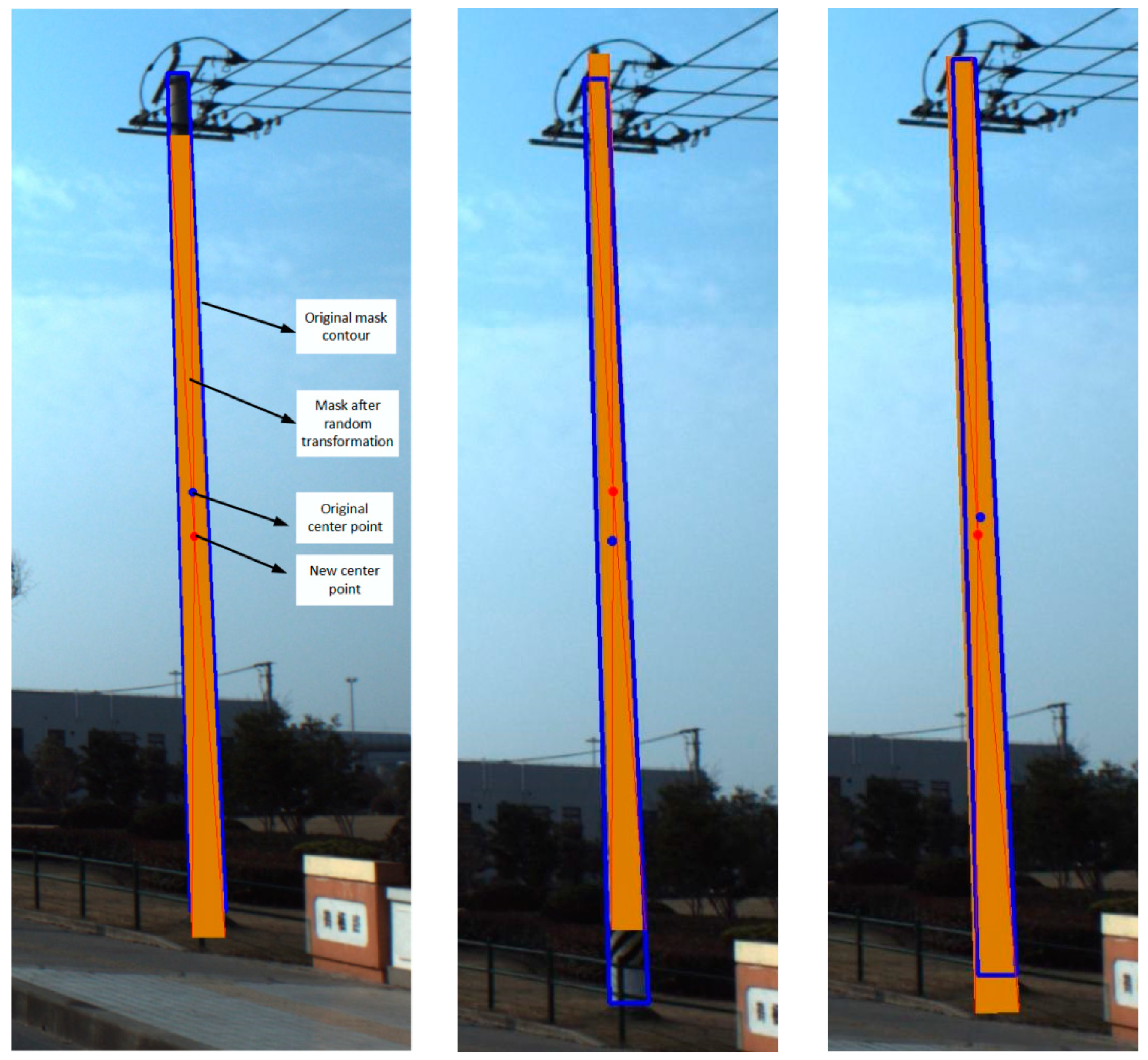
2.3.1. Labeling Mask Random Transform

The random transformation of the mask is realized by randomly changing the center point position and outline size of the mask. The principle of random transformation is shown in Figure 7. The process is as follows.

Equation (4) is used to calculate the original center point position, the distance and slope of the line connecting the center point, and the contour point. The original center point position refers to the average coordinate position of all contour points.

$$\begin{gathered} \left\{\begin{array}{c}{x}_0=\frac{1}{n}{\displaystyle \sum _{i=1}^n}{x}_i\\ y_0=\frac{1}{n}{\displaystyle \sum _{i=1}^n}{y}_i\end{array}\right. \\ {d}_0=\sqrt{{\left(x_0-x_i\right)}^2+{\left(y_0-y_i\right)}^2} \\ {k}_0=\left(y_i-y_0\right)/\left(x_i-x_0\right) \end{gathered}$$

(4)

where, $\left(x_0 ,y_0\right)$ is the coordinate position of the center point,$\left(x_i ,y_i\right)$ is the coordinate position of the contour point, $d_0$ is the distance from the center point to the contour point, and $k_0$ is the slope of the line connecting the center point and the contour point.

(1) The center point position, distance and slope are randomly transformed by Equation (5).

$$\begin{gathered} \left\{\begin{array}{c}{x}_{n0}=x_0+r_0\times w ,r_0\in \left(-0.1,0.1\right)\\ y_{n0}=y_0+r_0\times h, r_0\in \left(-0.1,0.1\right)\end{array}\right. \\ {d}_n=d_0\times r_1, r_1\in \left(0.9,1.1\right) \\ {k}_n=k_0\times r_1, r_1\in \left(0.9,1.1\right) \end{gathered}$$

(5)

where, $\left(x_{n0},y_{n0}\right)$ is the coordinate position of the center point after the transformation, $d_n$ and $k_n$ are the distance and slope after the transformation, respectively.

(2) The new contour point coordinates from the transformed center point, slope, and distance are calculated as Equation (6):

$$\left\{\begin{array}{l}{d}_n=\sqrt{{\left(x_{ni}-x_{n0}\right)}^2+{\left(y_{ni}-y_{n0}\right)}^2}\\ k_n=\left(y_{ni}-y_{n0}\right)/\left(x_{ni}-x_{n0}\right) \end{array}\right.$$

(6)

where, $\left(x_{ni} ,y_{ni}\right)$ is the coordinate position of the transformed contour point.

Figure 8 shows the results of the random transformation of the pole mask. The blue box is the original mask contour, and the orange part is the random transformed mask.

2.3.2. 3D Reconstruction of Utility Poles

The transformation of the world coordinate system, camera coordinate system, image coordinate system, and pixel coordinate system will be involved in the generation of the pole. In Figure 9, $P_w$ is a point in space, which is represented by ($X_{Pw}$, $Y_{Pw}$, $Z_{Pw}$) in the world coordinate system and ($X_{PC}$, $Y_{PC}$, $Z_{PC}$) in the camera coordinate system. The point $P_w$ on the imaging plane is denoted by p, which is represented as $\left(x,y\right)$ in the image coordinate system and (u, v) in the pixel coordinate system.

The spatial point $P_w$ ($X_{Pw}$, $Y_{Pw}$, $Z_{Pw}$) in the world coordinate system can be transformed into the imaging point p (u, v) in the pixel coordinate by the transformation matrix, as shown in Equation (7).

$$Z_{PC}\left[\begin{array}{c}u\\ v\\ 1\end{array}\right]=\left[\begin{array}{c}\frac{1}{dx} 0 u_0\\ 0 \frac{1}{dy} v_0\\ 0 0 1 \end{array}\right]\left[\begin{array}{c}f 0 0 0\\ 0 f 0 0\\ 0 0 1 0\end{array}\right]\left[\begin{array}{c}R t\\ 0^T 1\end{array}\right]\left[\begin{array}{c}{X}_{Pw}\\ Y_{Pw}\\ Z_{Pw}\\ 1\end{array}\right]$$

(7)

where, dx and dy represent the actual physical size of a single pixel along the x-axis and y-axis, $\left(u_0,v_0\right)$ is the coordinate value of the camera coordinate system origin o in the pixel coordinate system, f represents the camera focal length, and R and t represent the rotation matrix and offset vector converted from the world coordinate system to the camera coordinate system, respectively.

Similarly, combined with the depth information provided by the depth map, the pixel points provided by the pole mask can be transformed into the spatial points in the world coordinate system by using the transformation matrix, and the frustum point cloud containing the poles and interference points can be obtained. Figure 10 illustrates the transformation results.

2.4. Utility Pole Point Cloud Segmentation

2.4.1. Preprocessing

The frustum point cloud obtained by the 3D reconstruction still contains some background interference points. Before the point cloud segmentation, preprocessing is performed to remove noise and enhance features for the segmentation. The processing method is as follows.

(1) Because the statistical filter has a better effect on the removal of outliers with large density differences, the statistical filter is used to filter the frustum point cloud. The principle of the statistical filter is as follows. Calculate the average distance $d_i$ from each point to the k points in the neighborhood. The average distance of all point clouds conforms to the Gaussian distribution. A distance threshold $d_{max}$ is set by the mean $\mathsf{\mu }$ and standard $\mathsf{\sigma }$ deviation of the Gaussian distribution. Points whose average distance exceeds the distance threshold are defined as outliers $outlie{r}_i$. The statistical filter can be written as

$$d_i=\frac{1}{k}{\displaystyle \sum }_{j=1}^k\sqrt{{\left(x_{ij}-x_i\right)}^2+{\left(y_{ij}-y_i\right)}^2+{\left(z_{ij}-z_i\right)}^2}$$

(8)

$$\mathsf{\mu }=\frac{1}{n}{\displaystyle \sum }_1^n{d}_i$$

(9)

$$\mathsf{\sigma }=\sqrt{\frac{1}{n}{\displaystyle \sum }_1^n{\left(d_i-\mu \right)}^2}$$

(10)

$$d_{max}=\mu \pm \alpha ·\sigma$$

(11)

$$outlie{r}_i=\left\{\begin{array}{l}true, d_i>d_{max}\\ false, others\end{array} \right.$$

(12)

where, $\left(x_i ,y_i ,z_i\right)$ represents the coordinate of any point in the point cloud, $\left(x_{ij} ,y_{ij} ,z_{ij}\right)$ represents the coordinate of any adjacent point among the k points in the neighborhood, n represents the number of point clouds, and $\mathsf{\alpha }$ represents the standard deviation coefficient.

(2) The visible point is determined from the viewpoint position, and the color is added to the visible point, which can not only increase the color feature of the pole and improve the point cloud recognition rate, but also distinguish the pole and the noise point, which is conducive to the point cloud labeling.

(3) The down sampling process can reduce the density of the point cloud. In order to ensure that the point cloud after down sampling maintains the original structure as much as possible, a uniform down sampling method is used. The number of frustum point clouds varies, which is inconvenient as an input sample for the PointNet model. Randomly select N point from the point cloud for a fixed number, and repeat the selection when the number of point clouds is less than N.

(4) Normalization can accelerate the convergence speed of the model. The frustum point cloud contains 6 dimensions (x, y, z, r, g, b), and the point cloud is normalized using Equation (13).

$$\left\{\begin{array}{l}{x}_1=\frac{x_0-\mu }{\sigma }\\ c_1=c_0/255 \end{array}\right.$$

(13)

where, $x_0$ represents the position (x, y, z) data of the original coordinate point, $x_1$ represents the position data of the normalized coordinate point, $\mu$ is the mean of the original coordinate point position data, $\sigma$ is the variance of the original coordinate point position, $c_0$ represents the color of the original coordinate point (r, g, b) data, $c_1$ representing normalized color data.

Here, k is set to 20, and $\mathsf{\alpha }$ is set to 2. The down sampling multiple is 5. After down sampling, the original point cloud of about 25 k is reduced to about 5 k. N = 4096 is selected as the fixed number of point clouds. Figure 11 shows the intermediate process of preprocessing.

2.4.2. PointNet Point Cloud Segmentation

The instance segmentation of the pole images has been classified into categories; therefore, point cloud segmentation only needs to distinguish the foreground and background. Although Pointnet [33] is a lightweight network model, it has achieved good results in both point cloud classification and point cloud segmentation. Considering the segmentation speed and accuracy requirements, PointNet is selected as the point cloud segmentation model. Figure 12 shows the PointNet point cloud segmentation model. The preprocessed frustum is input. Firstly, the MLP network is used to gradually upgrade the point cloud from 6 (x, y, z, r, g, b) dimensions to a high-dimensional space of 1024 dimensions, in which two T-Net networks are introduced to solve the point cloud rotation invariance problem. Then, the Max Pooling is taken as a symmetric function to extract the global features of the point cloud. Finally, the local features of each point are fused with the global features, and then the point cloud dimension is gradually reduced to two dimensions through MLP again.

During data acquisition, the poles probably exist on the left and right sides of the acquisition device, so there are the pole point cloud data in the positive and negative intervals of the camera coordinate system. Compared to the rectified linear unit (ReLU) function, the leaky ReLU (LReLU) function has a relatively small slope $\mathsf{\alpha }$ on the negative axis, as shown in Equations (14) and (15). To avoid the disappearance of the gradient, LReLU replaces the ReLU activation function as the intermediate layer activation function. The activation function of the output layer uses the Sigmoid function and the binary cross entropy loss function is applied to calculate the loss, which is calculated as Equation (16).

$$ReLU\left(x\right)=\left\{\begin{array}{l}x, x>0\\ 0 , x\le 0\end{array}\right.$$

(14)

$$LReLU\left(x\right)=\left\{\begin{array}{l}x, x>0\\ \alpha x, x\le 0\end{array}\right.$$

(15)

$$Loss=-\frac{1}{n}\left[{\displaystyle \sum }_{i=1}^n{y}_i\log y_i^{\prime }+\left(1-y_i\right)\log \left(1-y_i^{\prime }\right)\right]$$

(16)

where, i represents the ith sample, n represents the number of samples, $y_i$ represents the true label value, $y_i^{\prime }$ represents the predicted value, and Loss represents the loss value.

2.5. Pole Central Axis Fitting and Angle Calculation

The shape of the outer contour of the pole is mostly an approximate cone or cylinder. The pole point cloud is a set of point clouds with an outer contour of half arc surface and inclination in any direction of space. It is difficult to directly fit the regular geometric model to obtain an accurate central axis. Hence, the method of piecewise fitting is implemented to obtain the central axis of the pole point cloud and calculate the inclination angle. The specific steps are as follows:

(1) The pole point cloud is divided in the height direction (Y-axis), and then the point cloud data is cut out in two planes every 0.5 meters along the Y-axis direction, and each piece of the segmented data is processed separately.

(2) Each intercepted point cloud is processed into a cylinder model, which is fitted using the RANSAC algorithm [34]. The basic flow of the algorithm is as follows:

Step 1: Randomly select n points from the sample data set to construct the initial model. Generally, the least mean square algorithm is used to calculate the model parameters, where n needs satisfy the minimum data required for the model, for the cylinder model, n > 6.

Step 2: The constructed model is used to test other data points, then the deviation of all sample points from the model is calculated. Set a threshold T. Next, the sample points whose deviation is less than the threshold T are considered as inner points, otherwise, they are considered as outer points.

Step 3: Only the more accurate model is retained according to the number of interior points and the error rate of the model.

Step 4: Repeat the above steps until the set number of iterations k is met.

Here, n is set to 100, T is set to 0.3, and k is set to 10,000, experimentally. In addition, the estimated radius of the cylinder R is set to 0–3, and the distance weight of the surface normal is set to 0.2. After the RANSAC algorithm iteration, the output result is an inner point set with noise-free and seven model parameters including the position coordinate (x, y, z) of a point on the axis, the axis direction vector $\left(\overrightarrow{x},\overrightarrow{y},\overrightarrow{z}\right)$, and the cylinder radius R. The parameters uniquely determine a cylinder model, and then the coordinates of any other point on the axis can be expressed as Equation (17). Select five points equidistant from the axis of each section as the center point.

$$\left\{\begin{array}{l}{x}_1=x+t\times \overrightarrow{x}\\ y_1=y+t\times \overrightarrow{y}\\ z_1=z+t\times \overrightarrow{z}\end{array}\right.$$

(17)

where, $\left(x_1,y_1,z_1\right)$ is the position coordinate of any point on the axis, t is a constant, which is determined by the intercepted interval position and the number of selected points.

(3) Referring to the space linear equation, as shown in Equation (18), the least squares method is used to fit the spatial straight line for the center points obtained by all the segments [35], which is expressed as Equation (19), and the fitted spatial straight line is the central axis of the pole.

The fitting results of the central axis of the pole are shown in Figure 13.

$$\frac{x_i-x_0}{m}=\frac{y_i-y_0}{n}=\frac{z_i-z_0}{p}$$

(18)

$$\left[\begin{array}{cc}m& x_0\\ n& y_0\end{array}\right]=\left[\begin{array}{cc}\sum x_i{z}_i& \sum x_i\\ \sum y_i{z}_i& \sum y_i\end{array}\right]{\left[\begin{array}{cc}\sum z_i{}^2& \sum z_i\\ \sum z_i& n\end{array}\right]}^{-1}$$

(19)

(4) Arbitrarily take two points on the central axis of the pole, and use Equation (20) to calculate the inclination angle of the pole.

$$\mathsf{\theta }={90}^{°}-\arctan \left(\frac{Y_2-Y_1}{\sqrt{{\left(X_2-X_1\right)}^2+{\left(Z_2-Z_1\right)}^2}}\right)\times \frac{180}{\pi }$$

(20)

where, $(X_1,Y_1,Z_1)$, $(X_2,Y_2,Z_2)$ are the coordinate values of the two points on the central axis, respectively.

3. Experiment and Analysis

3.1. Datasets

This study uses the open-source dataset ApolloScape [36]. Compared to real-world datasets such as KITTI or Cityscapes [37], ApolloScape contains larger and richer scenes and the point clouds generated by LiDAR are more dense, which contains a large number of complete roadside objects such as signboards, street lamps, and utility poles, providing RGB images with a resolution of 3384 × 2710 pixels and corresponding depth maps. When training the image segmentation model, 3000 pictures containing utility pole objects are selected as the data set, of which, 2000 are used as training sets, 500 are used as test sets and 500 are used as verification sets.

When training the pole point cloud segmentation model, 5000 frustums generated by the pole mask and depth map were selected, of which, 3000 were used for training, 1000 for test set and 1000 for verification set, and frustums were annotated by CloudCompare software.

3.2. Model Training

The experiment was performed on an Inspurserver with operating system UBUNTU18.04 and two NVIDIA Tesla T4 16G GPUs. The deep learning framework was TensorFlow1.15.0. The COCO dataset contains complex scenes of common objects in the natural environment, which is often used for object detection and instance segmentation [38]. The improved Mask R-CNN is transfer learning based on the pre-trained weights for the COCO dataset. The image resolution is adjusted to 1024 × 1024 (pixels). Stochastic gradient descent was performed with the stochastic gradient descent with momentum (SGDM) optimizer, of which, a batch size is 2, an initial learning rate is 0.001, and a momentum factor is 0.9. The head network is trained for 20 epochs, and all network layers are trained for 40 epochs. ResNet50-FPN, ResNet101-FPN, and ResNet152-FPN backbone networks were used for testing, respectively [39]. From the training results in Figure 14, it is found that the loss curve of ResNet101-FPN has the best convergence effect, and the loss is reduced to less than 0.2. Therefore, ResNet101-FPN is selected as the backbone network of the model.

The open-source SUN-RGBD dataset is a large-scale 3D dataset with dense annotations, often used for scene understanding [40]. When training PointNet, the SUN-RGBD dataset label is first modified to retain only the foreground and background, and then it is used to pre-train PointNet to enable the network to perform feature extraction. On this basis, the manually annotated frustum point cloud is trained, and gradient descent using adaptive moments estimation (Adam) optimizer with batch size 8 is used. An exponential decay learning rate is adopted, the initial learning rate is 0.001, the decay period is 300,000 steps, and the decay rate is 0.5. A total of 50 epochs were trained. In Figure 15, the Loss curve and Accuracy curve of the training process show that the loss value decreases rapidly at the beginning of training, the accuracy rate increases rapidly, and then gradually stabilizes. Finally, the loss value decreases to less than 0.2, and the accuracy rate gradually increases to about 94%.

3.3. Model Evaluation and Result Analysis

The Mask R-CNN model is evaluated by average precision (AP). AP refers to the area surrounded by precision-recall (P-R) curves and coordinates under a certain intersection union ratio (IoU), which is used to represent the average correctness of detection under different recall rates. For example, AP₅₀ represents the value of AP when the IoU threshold is 0.5. The recall rate (R), precision (P), and AP are displayed as

$$R=\frac{TP}{TP+FN}$$

(21)

$$P=\frac{TP}{TP+FP}$$

(22)

$$AP={{\displaystyle \int }}_0^{1}Prdr$$

(23)

where, TP represents the part correctly predicted as the pole, FN represents the part where the pole is incorrectly predicted as the background, and FP represents the part where the background is incorrectly predicted as the pole. P(r) refers to the P-R curve.

Table 1. Comparison of segmentation effect.

Method	P	R	AP50	AP75
Mask R-CNN	63.3%	99.25%	90.55%	6.58%
Mask R-CNN + box expanded	93.16%	99.5%	90.11%	57.05%
Mask R-CNN + CBAM	67.23%	95.3%	90.62%	8.03%
Mask R-CNN + box expanded + CBAM	95.03%	99.7%	91.13%	58.15%

shows the experimental results. The accuracy of the original Mask R-CNN for pole skeleton segmentation is relatively low, and the AP₇₅ is significantly lower when the IoU is at a high threshold of 0.75. Compared with the original Mask R-CNN, the segmentation accuracy after expanding bounding box has been significantly improved. Among them, P is increased by 30%, and AP₇₅ is increased by 50%, which proves that the correction of the bounding box has a greater impact on the segmentation accuracy. Only adding the CBAM attention mechanism can improve the detection effect of the pole to a certain extent. The combination of bounding box modified and CBAM attention mechanism has the best effect with AP₅₀ and AP₇₅, improving by 1% and 52%, respectively. When the IoU is 0.5, P and R increase by 32% and 0.5%, respectively, which reduces the error rate of pole recognition and increases the accuracy of pole segmentation.

The test effects of the original model and the improved model are intuitively shown in Figure 16.

The point cloud segmentation effect is evaluated by accuracy (ACC) and IoU. After training, the accuracy and intersection over union of PointNet segmentation are 92.4% and 83.7%, respectively. ACC and IoU can be obtained from the following equations.

$$ACC=\frac{P{C}_t}{P{C}_p}$$

(24)

$$IoU=\frac{P{C}_t}{P{C}_p+P{C}_{gt}-P{C}_t}$$

(25)

where, $P{C}_t$ is the number of point clouds correctly predicted as the poles, $P{C}_p$ is the number of point clouds predicted as the poles, and $P{C}_{gt}$ is the number of point clouds that actually contain pole.

After the central axis fitting and angle calculation, the overall detection results are shown as Figure 17, where the detected angle is the inclination angle in the camera coordinate system.

3.4. Angle Verification and Analysis

3.4.1. Experimental Environment

In order to verify the correctness of the measurement of the pole from different observation directions at a fixed inclination angle, a pole model for simulation was designed and built in the laboratory. The depth camera Percipio DS460 is used to obtain the depth map of the pole.

The pole is fixed on the inclined platform, and the camera is adjusted to the horizontal position. For simplified calculation, the camera coordinate system and the world coordinate system are set to the same coordinate system. The inclination angle is adjusted by the inclined platform every 2° from 0–10° and the observation direction is adjusted by rotating the platform every 45° in a clockwise direction from 0–360°. The average value of five measurements is taken as the final result of this inclination angle and observation direction. The experimental environment is shown in Figure 18. Where, 1. pole model, 2. depth camera, 3. image processing system, 4. rotating platform, 5. inclined platform, and 6. angle measuring instrument.

3.4.2. Processing

The intermediate process is shown as Figure 19. Firstly, the collected depth map is manually segmented and the pole skeleton is randomly transformed. Then, using the camera projection matrix, the frustum is generated through 3D reconstruction and the pole point cloud is obtained after the frustum is preprocessed and segmented by the PointNet. Finally, the central axis of the pole is fitted, and then the inclination angle is obtained.

3.4.3. Analysis of Experimental Results

The error range of the inclination angle of the pole is 0–1.35°, the average error is 0.66°, and the variance is 0.12° (

Table 2. Pole angle distribution.

Inclination Angle	Rotation Angle								Average Error	Variance
	0	45	90	135	180	225	270	315
0	0.91	0.35	0.82	0.45	0.65	1.15	0.32	1.14	0.72	0.11
2	2.35	2.34	2.65	2.42	2.85	2.32	3.35	2.92	0.65	0.14
4	4.33	4.27	4.53	5.15	4.71	4.53	5.12	5.07	0.71	0.13
6	6.56	6.69	6.05	6.74	7.32	6.15	7.13	6.32	0.62	0.20
8	8.35	8.86	8.44	9.13	8.62	8.81	8.06	8.78	0.63	0.11
10	10.53	10.36	10.94	10.43	10.52	11.11	10.84	10.13	0.61	0.11

). Under the same inclination angle and different observation directions, the average error range of detection is 0.61°–0.72°. Among them, there is a maximum error of 1.35° when the inclination is 2° and the observation direction is 270°. One possible reason is that the inclination angle error is affected by the measurement error of the angle sensor and remote observation error of the depth camera. The variance range is 0.11°–0.2° under different observation directions at the same inclination angle, the reason for which is that under different observation angles, the distribution of pole objects and background interference points in the frustum generated by the mask fusion depth map are different, so the segmented pole point cloud is naturally different, which eventually leads to the difference in the inclination angle calculated by the central axis fitting.

4. Conclusions

A new method using 2D image and 3D point cloud to estimate the inclination angle of a pole has been proposed. The method has the following features:

• The expanded bounding box and the attention mechanism are the main influencing factors for improving Mask R-CNN in pole detection. It effectively executes to locate the pole by reducing the searching space in the 3D point cloud.
• It can segment high-quality pole data from the raw point cloud by introducing the pole mask feature and depth map fusion.
• It can estimate the inclination angle of the pole point cloud by fitting the central axis of the cylinder-like objects, even in scenarios of noise or missing point cloud.

The method could be improved by:

• As the quality of the pole visible light (RGB) image could be insufficient in variable light, such as strong sunlight or rain, the improved Mask R-CNN might not accurately detect the pole. The preprocessing step of enhancing the RGB image is necessary for the automatic detection method.
• As the unmatched 2D image is captured from a visible light camera and the 3D point cloud is captured from LiDAR or a depth camera, the reduced point cloud searching space in the new method might not able to locate the pole.

In the future, the present study will be extended to optimize the algorithm running speed on edge computing devices for large-scale pole inclination angle estimations in a city.

References

1. Meng, W.; Dai, Z.; Chen, Y.; Huang, Y.; Li, X. Research on active safety protection technology of distribution network poles. Ind. Saf. Environ. Prot. 2022, 48, 74–76 + 106. [Google Scholar]
2. Luo, J.; Yu, C.; Xie, Y.; Chen, B.; Huang, W.; Cheng, S.; Wu, Y. Review of power system security and stability defense methods under natural disasters. Power Syst. Prot. Control 2018, 46, 158–170. [Google Scholar]
3. Zhang, X.; Wang, N.; Wang, W.; Feng, J.; Liu, X.; Hou, K. Resilience assessment of power systems considering typhoon weather. Proc. CSU-EPSA 2019, 31, 21–26. [Google Scholar]
4. Wang, Y.; Yin, Z.; Li, L.; Wang, X.; Zhang, G.; Mu, Y. Risk assessment method for distribution network considering operation status under typhoon disaster scenario. Proc. CSU-EPSA 2018, 30, 60–65. [Google Scholar]
5. Liang, Q.; Liang, S.; Peng, J.; Bian, M. Wind-Resistant monitoring technology of pole-line structure in transmission lines. J. Electr. Power Sci. Technol. 2020, 35, 181–186. [Google Scholar]
6. Kim, J.; Kamari, M.; Lee, S.; Ham, Y. Large-scale visual data–driven probabilistic risk assessment of utility poles regarding the vulnerability of power distribution infrastructure systems. J. Constr. Eng. Manag. 2021, 147. [Google Scholar] [CrossRef]
7. Li, Y.; Du, Y.; Shen, X.; Wang, R. Comparison of several transmission line tower inclination measurement methods. Hubei Electr. Power 2014, 38, 55–57 + 74. [Google Scholar]
8. Wang, S.; Du, Y.; Sun, J.; Fang, Q.; Weng, Y.; Ma, L.; Zhang, X.; Wu, J.; Qin, Q.; Shi, Q. Transmission tower deformation and tilt detection research status. Telecom Power Technol. 2018, 35, 91–92. [Google Scholar] [CrossRef]
9. Tragulnuch, P.; Kasetkasem, T.; Isshiki, T.; Chanvimaluang, T.; Ingprasert, S. High voltage transmission tower detection and tracking in aerial video sequence using object-based image classification. In Proceedings of the International Conference on Embedded Systems and Intelligent Technology (ICESIT)/International Conference on Information and Communication Technology for Embedded Systems (ICICTES), Khon Kaen, Thailand, 7–9 May 2018. [Google Scholar]
10. Yang, Y.; Chen, Y.; Chen, Y.; Xiao, F.; He, W. A new method of retrieving the inclination direction of power transmission tower by geocoding. In Proceedings of the 38th IEEE International Geoscience and Remote Sensing Symposium (IGARSS), Valencia, Spain, 22–27 July 2018. [Google Scholar]
11. Li, L.; Gao, X.; Liu, W. On-line monitoring method of transmission tower tilt based on remote sensing satellite optical image and neural network. In Proceedings of the 11th International Conference on Power and Energy Systems (ICPES), Shanghai, China, 18–20 December 2021. [Google Scholar]
12. Alam, M.M.; Zhu, Z.; Tokgoz, B.E.; Zhang, J.; Hwang, S. Automatic assessment and prediction of the resilience of utility poles using unmanned aerial vehicles and computer vision techniques. Int. J. Disaster Risk Sci. 2020, 11, 119–132. [Google Scholar] [CrossRef] [Green Version]
13. Mo, Y.F.; Xie, R.; Pan, Q.; Zhang, B. Automatic power transmission towers detection based on the deep learning algorithm. In Proceedings of the 2nd International Conference on Computer Engineering and Intelligent Control (ICCEIC), Chongqing, China, 12–14 November 2021. [Google Scholar]
14. Zhang, W.; Witharana, C.; Li, W.; Zhang, C.; Li, X.; Parent, J. Using deep learning to identify utility poles with crossarms and estimate their locations from google street view images. Sensors 2018, 18, 2484. [Google Scholar] [CrossRef] [Green Version]
15. Gomes, M.; Silva, J.; Goncalves, D.; Zamboni, P.; Perez, J.; Batista, E.; Ramos, A.; Osco, L.; Matsubara, E.; Li, J.; et al. Mapping utility poles in aerial orthoimages using ATSS deep learning method. Sensors 2020, 20, 6070. [Google Scholar] [CrossRef] [PubMed]
16. Hosseini, M.; Umunnakwe, A.; Parvania, M.; Tasdizen, T. Intelligent damage classification and estimation in power distribution poles using unmanned aerial vehicles and convolutional neural networks. IEEE Trans. Smart Grid 2020, 11, 3325–3333. [Google Scholar] [CrossRef]
17. Lu, Z.; Gong, H.; Jin, Q.; Hu, Q.; Wang, S. A transmission tower tilt state assessment approach based on dense point cloud from UAV-Based LiDAR. Remote Sens. 2022, 14, 408. [Google Scholar] [CrossRef]
18. Chen, M.; Chan, T.; Wang, X.; Luo, M.; Lin, Y.; Huang, H.; Sun, Y.; Cui, G.; Huang, Y. A risk analysis framework for transmission towers under potential pluvial flood—LiDAR survey and geometric modelling. Int. J. Disaster Risk Reduct. 2020, 50, 14. [Google Scholar] [CrossRef]
19. Wang, Y.; Han, J.; Zhao, Q.; Wang, Y. The method of power transmission tower inclination detection based on UAV image. Comput. Simul. 2017, 34, 426–431. [Google Scholar]
20. Shi, Z.; Kang, Z.; Lin, Y.; Liu, Y.; Chen, W. Automatic recognition of Pole-Like objects from mobile laser scanning point clouds. Remote Sens. 2018, 10, 1891. [Google Scholar] [CrossRef] [Green Version]
21. Kang, Z.; Yang, J.; Zhong, R.; Wu, Y.; Shi, Z.; Lindenbergh, R. Voxel-Based extraction and classification of 3-D Pole-Like objects from mobile LiDAR point cloud data. IEEE J. Sel. Top. Appl. Earth Observ. Remote Sens. 2018, 11, 4287–4298. [Google Scholar] [CrossRef]
22. Teo, T.A.; Chiu, C.M. Pole-Like road object detection from mobile lidar system using a Coarse-to-Fine approach. IEEE J. Sel. Top. Appl. Earth Observ. Remote Sens. 2015, 8, 4805–4818. [Google Scholar] [CrossRef]
23. Ha, T.; Chaisomphob, T. Automated localization and classification of expressway Pole-Like road facilities from mobile laser scanning data. Adv. Civ. Eng. 2020, 2020, 18. [Google Scholar]
24. Tian, X.; Wang, L.; Ding, Q. A review of image semantic segmentation methods based on deep learning. J. Softw. 2019, 30, 440–468. [Google Scholar]
25. Su, L.; Sun, Y.; Yuan, S. A review of case segmentation based on deep learning. CAAI Trans. Intell. Syst. 2022, 17, 16–31. [Google Scholar]
26. He, K.; Gkioxari, G.; Dollar, P.; Girshick, R. Mask r-cnn. In Proceedings of the 16th IEEE International Conference on Computer Vision (ICCV), Venice, Italy, 22–29 October 2017. [Google Scholar]
27. Zhang, J.; Zhao, X.; Chen, Z. Review of semantic segmentation of point cloud based on deep learning. Laser Optoelectron. Prog. 2020, 57, 28–46. [Google Scholar] [CrossRef]
28. Ma, C.; Huang, M. A unified cone, cone, cylinder fitting method. In Proceedings of the Ninth Beijing-Hong Kong-Macao Surveying and Mapping Geographic Information Technology Exchange Conference, Beijing, China, 6–7 November 2015. [Google Scholar]
29. Ghiasi, G.; Lin, T.; Le, Q.V.; Soc, I.C. Nas-fpn: Learning scalable feature pyramid architecture for object detection. In Proceedings of the 32nd IEEE/CVF Conference on Computer Vision and Pattern Recognition (CVPR), Long Beach, CA, USA, 16–20 June 2019. [Google Scholar]
30. Long, J.; Shelhamer, E.; Darrell, T. Fully convolutional networks for semantic segmentation. In Proceedings of the IEEE Conference on Computer Vision and Pattern Recognition (CVPR), Boston, MA, USA, 7–12 June 2015. [Google Scholar]
31. Woo, S.H.; Park, J.; Lee, J.Y.; Kweon, I.S. Cbam: Convolutional block attention module. In Proceedings of the 15th European Conference on Computer Vision (ECCV), Munich, Germany, 8–14 September 2018. [Google Scholar]
32. Qi, C.; Liu, W.; Wu, C.; Su, H.; Guibas, L.J. Frustum pointnets for 3D object detection from RGB-D data. In Proceedings of the 31st IEEE/CVF Conference on Computer Vision and Pattern Recognition (CVPR), Salt Lake City, UT, USA, 18–23 June 2018. [Google Scholar]
33. Qi, C.; Su, H.; Mo, K.C.; Guibas, L.J. Pointnet: Deep learning on point sets for 3d classification and segmentation. In Proceedings of the 30th IEEE/CVF Conference on Computer Vision and Pattern Recognition (CVPR), Honolulu, HI, USA, 21–26 July 2017. [Google Scholar]
34. Brachmann, E.; Rother, C. Neural-Guided RANSAC: Learning where to sample model hypotheses. In Proceedings of the IEEE/CVF International Conference on Computer Vision (ICCV), Seoul, Republic of Korea, 27 October–2 November 2019. [Google Scholar]
35. Cui, L.; Yang, R.; Qian, J.; Zhang, H.; Chen, K. Spatial linear fitting algorithm based on total least squares. J. Chengdu Univ. 2019, 38, 102–105. [Google Scholar]
36. Huang, X.; Wang, P.; Cheng, X.; Zhou, D.; Geng, Q.; Yang, R. The apolloscape open dataset for autonomous driving and its application. IEEE Trans. Pattern Anal. Mach. Intell. 2020, 42, 2702–2719. [Google Scholar] [CrossRef] [PubMed] [Green Version]
37. Peng, Y.; Zheng, W.; Zhang, J. Summarization of 3D object detection methods based on deep learning. Automob. Technol. 2020, 540, 1–7. [Google Scholar] [CrossRef]
38. Lin, T.-Y.; Maire, M.; Belongie, S.; Hays, J.; Perona, P.; Ramanan, D.; Dollár, P.; Zitnick, C.L. Microsoft COCO: Common objects in context. In European Conference on Computer Vision (ECCV), Zurich, Switzerland, 6–12 September 2014; Springer: Cham, Switzerland, 2014; pp. 740–755. [Google Scholar]
39. He, K.; Zhang, X.; Ren, S.; Sun, J. Deep residual learning for image recognition. In Proceedings of the 2016 IEEE Conference on Computer Vision and Pattern Recognition (CVPR), Las Vegas, NV, USA, 27–30 June 2016; pp. 770–778. [Google Scholar]
40. Song, S.; Lichtenberg, S.P.; Xiao, J. Sun rgb-d: A rgb-d scene understanding benchmark suite. In Proceedings of the IEEE Conference on Computer Vision and Pattern Recognition, Boston, MA, USA, 7–12 June 2015; pp. 567–576. [Google Scholar]
Figure 1. Overall detection process.
Applsci 13 01688 g001
Figure 2. Network structure of the improved Mask R-CNN.
Applsci 13 01688 g002
Figure 3. Expanding bounding box. (a) The structure of the pole; (b) Bounding box expansion; (c) Bounding box expanding to different values according to . In this case, the red line represents the original bounding box and the blue line represents the expanded bounding box. The left side is expanded by 0.51 w 0 and the right side by 1.33 w 0 in the width direction of the original bounding box.
Applsci 13 01688 g003
Figure 4. Comparison of original bounding box and expanded bounding box.
Applsci 13 01688 g004
Figure 5. CBAM attention mechanism.
Applsci 13 01688 g005
Figure 6. Head network of Mask R-CNN with attention mechanism introduced.
Applsci 13 01688 g006
Figure 7. Schematic diagram of mask transformation principle.
Applsci 13 01688 g007
Figure 8. Mask random transformation results.
Applsci 13 01688 g008
Figure 9. Coordinate system transformation.
Applsci 13 01688 g009
Figure 10. 3D reconstruction results.
Applsci 13 01688 g010
Figure 11. Point cloud preprocessing. (a) The frustum generated by the mask and depth map, where the pole points are in the red dot line box; (b) The illustration of the noise filter processing. In this case, the red points are noise; (c) Adding color (blue) from viewpoint direction.
Applsci 13 01688 g011
Figure 12. Network structure of PointNet.
Applsci 13 01688 g012
Figure 13. The fitting result of the central axis of the pole. (a) Point cloud intercepted; (b) RANSAC fitting cylinder; (c) Central axis fitted.
Applsci 13 01688 g013
Figure 14. Loss curve of image segmentation training.
Applsci 13 01688 g014
Figure 15. Point cloud segmentation training process. (a) Loss curve; (b) Accuracy curve.
Applsci 13 01688 g015
Figure 16. Visual display of original and improved effects. (a) Original Mask R-CNN segmentation effect; (b) Improved Mask R-CNN segmentation effect.
Applsci 13 01688 g016
Figure 17. Pole angle measurement. (a) RGB image; (b) Pole point cloud segmentation results; (c) Measurement results in the camera coordinate system.
Applsci 13 01688 g017
Figure 18. The experimental environment of the simulated pole. Where, 1. pole model, 2. depth camera, 3. image processing system, 4. rotating platform, 5. inclined platform, and 6. angle measuring instrument.
Applsci 13 01688 g018
Figure 19. Intermediate process of the pole inclination angle. (a) Pole depth map; (b) Image segmentation; (c) Frustum point cloud; (d) Preprocessing and segmentation; (e) Pole segmentation results, where the pole points are in the white dot line box; (f) Central axis fitting.
Applsci 13 01688 g019