Abstract
Alongside the modern software development life cycle approaches, software testing has gained more importance and has become an area researched actively within the software engineering discipline. In this study, machine learning and deep learning-related software fault predictions were made through a data set named SFP XP-TDD, which was created using three different developed software projects. A data set of five different classifiers widely used in the literature and their Rotation Forest classifier ensemble versions were trained and tested using this data set. Numerous publications in the literature discussed software fault predictions through ML algorithms addressing solutions to different problems. Some of these articles indicated the usage of feature selection algorithms to improve classification performance, while others reported operating ensemble machine learning algorithms for software fault predictions. Besides, a detailed literature review revealed that there were few studies involving software fault prediction with DL algorithms due to the small sample sizes in the data sets and the low success rates in the tests performed on these datasets. As a result, the major contribution of this research was to statistically demonstrate that DL algorithms outperformed ML algorithms in data sets with large sample values via employing three separate software fault prediction datasets. The experimental outcomes of a model that includes a layer of recurrent neural networks (RNNs) were enclosed within this study. Alongside the aforementioned and generated data sets, the study also utilized the Eclipse and Apache Active MQ data sets in to test the effectiveness of the proposed deep learning method.
1. Introduction
The main objective of a software project is to deliver the expected functionality while meeting the required level of quality on time and within a defined budget [1]. From the perspective of software projects developed in recent years, the complexity in software development has increased due to the increased number of customer requirements. This complexity has made it more difficult for these projects to achieve their main objectives. The most important problems encountered in achieving said objectives are the faults presented within software. There are many studies conducted in software engineering that aim to develop effective methods for eliminating or reducing the number of these faults. These studies conducted for the development of software quality and management processes have led to the development of new approaches and methods with experimental investigations of successful software projects. In the discipline of software engineering, software metrics are heavily utilized in order to improve the quality of the software at hand owing to the significant insight they provide throughout the development process [2]. Using the best methods and tools available in the software development process does not guarantee that results will be free of faults. The most important method that can be used to detect software faults and to reduce their undesirable effects is testing the software in question. Software testing is the process of running a system or application under auditable conditions and evaluating the results obtained [3]. Insufficient testing of software projects may cause organizations to face major financial losses and in some cases may lead to human injuries or even massive deaths [4]. The duration and number of conducted tests heavily impact the successfulness of the tests at hand. If the software is tested insufficiently, various faults may remain undetected, leading to the presence of various undesirable behaviors in the future. Similarly, if the software is tested more than needed, the project cannot be completed within the expected time frame and the budget can also be exceeded due to the unexpected additional costs. Identification and correction of software faults in the early stages of development reduces the costs and risk of exceeding the predicted duration of the project. Developers are able to ascertain the fault susceptibility of the software by analyzing its code throughout the early stages of development with the effective use of software metrics. For software quality assurance, the early-stage prediction of software errors is crucial [5]. Numerous publications in the literature discussed software fault predictions through ML algorithms addressing solutions to different problems. Some of these articles indicated the usage of feature selection algorithms to improve classification performance [5,6], while others reported operating ensemble machine learning algorithms for software fault predictions [5]. Besides, a detailed literature review revealed that there were few studies involving software fault prediction with DL algorithms due to the small sample sizes in the datasets and the low success rates in the tests performed on these datasets [6]. As a result, the major contribution of this research was to statistically demonstrate that DL algorithms outperformed ML algorithms in data sets with large sample values via employing three separate software fault prediction datasets.
The application of the recurrent neural networks (RNN) based on the deep learning method developed in this study to the Eclipse and Apache Active MQ data sets, those frequently employed in software fault prediction studies, resulted in high-performance rates. Additionally, five different machine learning classifiers widely used in the literature and Rotation Forest (RF) classifier ensemble versions of these classifiers were executed on these data sets to compare the method performance. As Batool and Khan depicted in the conclusion section of their article, in which they collated roughly 70 different studies, they inferred that several data sets are necessary for the field of software fault prediction [6].
This study developed three separate software, including Accounting, Staffing, and Inventory software, using both the eXtreme Programming (XP) [7] software development methodology and the test-driven development (TDD) [8] approach to contribute to the resolution of this problem. These applications were developed by a development group consisting of seven people in the information technology department of a university. The software in question were used for over one year and their faults were recorded by a developed software management tool. A data set named SFP XP-TDD was created in order to make machine learning (ML) and deep learning (DL)-based software fault predictions. Data regarding some Chidamber and Kemerer (CK) metrics and other well- known metrics such as Cyclomatic Complexity, Comment Rate, Average Depth, Max Depth, Line Count, Statement Count, and Error Count [9] were obtained from these software. The primary motivation of this work is twofold: Initially, a novel software fault prediction data set named SFP XP-TDD was introduced to the literature and made publicly available for further studies in the field. Secondly, the study also provides the experimental outcomes of a model with a layer of recurrent neural networks (RNN). The study further used the SFP XP-TDD, Eclipse data sets [10], and the Apache Active MQ datasets [11] in addition to the data set developed to test the performance of the proposed deep learning method. Experimental results demonstrated that an RNN-based approach model is more accurate than many other machine learning and deep learning algorithms in software fault prediction. The study also provides the effectiveness of the Rotation Forest classifier ensemble in software fault prediction analyzed empirically. The rest of the paper is organized as follows: The Related Work section presents a comprehensive literature survey on software fault detection. In the Materials and Methods section, applied methods and algorithms in this study from machine learning and deep learning scope are introduced with their details. Then, the Experimental Results and Discussion section presents the experimental settings and results, and discusses the experimental results obtained, threads to validity. Finally, the paper is concluded with the Conclusions and Future Work section.
2. Related Work
The classification process is meant to assign given objects into relevant categories depending on predefined information and situations. To find the category of new incoming data, the category of previously collected data should be known [12]. A training model is built with the objects belonging to the known classes. The modules of the software code with faults can be predicted by using classification methods [13,14,15,16]. In the literature, classification algorithms such as decision trees, Bayesian classifiers, rule-based classifiers, artificial neural networks (ANN), k-nearest neighbor classifiers, support vector machines, and collective learning methods are frequently used. Moreover, several classification algorithms have been developed specifically for software fault prediction [17,18]. Many researchers have mentioned benefits of classification models for fault prediction [19,20]. In the literature, there are quite a number of studies regarding software fault prediction [21,22]. In 2009, Catal and Diri conducted studies related to fault predictions with Random
Forest, an ensemble machine learning algorithm, as well as algorithm-based artificial Immune systems. In this study, NASA’s public data sets were used. They determined that Random Forest (RF) had the highest performance in the large data sets. They also obtained the best area under receiver operating characteristics curve (AUC) values with Naive Bayes prediction algorithm for small data sets [18]. Arisholma, Briand, and Johannessen conducted software fault prediction using an old Java system in 2010. They determined that the impact of the collected pieces of data concerning correct predictions were limited, that process metrics are very useful for fault prediction, and that the best models are extremely dependent on the performance evaluation parameter. The usage of Adaboost combined with C4.5 alongside Weka’s default parameters yielded them the best results [23]. In a study by Cong Jin and Shu-Wei Jin in 2015, a hybrid method using ANN and quantum particle swarm optimization (QPSO) for software fault-proneness prediction was proposed. QPSO was used for reducing the dimensionality of the metrics data, and
ANN was used for predicting the fault-proneness of software modules. The proposed technique was shown to be effective for establishing a relationship between software metrics and fault-proneness [24]. Manjula and Florence used the Chidamber and Kemerer (CK) metrics in an experiment they conducted in 2019. They combined genetic algorithms (GA) and deep neural networks (DNN) for classification in their study, proposing a hybrid technique [25]. By experimenting in 2022, however, Nasir et al. developed a bidirectional encoder representations from transformers (BERT)-based semantic feature learning model and created a model called SDP-BB, which attempts to make software fault prediction [26].
Numerous studies have stated that ML algorithms developed for various objectives have also been used for software fault prediction. These articles additionally reported which ML algorithm solved software fault prediction better. For instance, while the article titled ‘Establishing a software defect prediction model via effective dimension reduction’ mentioned using the SVM algorithm to predict software faults, another article titled ‘Multiple-classifiers in software quality engineering: Combining predictors to improve software fault prediction ability’ cited using various prediction models, including Naïve Bayes (NB), Logistic Regression (LR), Support Vector Machine (SVM), K STAR, OneR (OR), and J48 [27].
The literature review has indicated that although there have not been as many publications referring to software fault prediction with ML algorithms, numerous studies have recently reported software fault prediction with DL algorithms. However, these studies utilized identical software metrics and prediction datasets previously used by ML algorithms. A review of the studies related to software fault prediction with the DL algorithms revealed the following: In the article titled ‘Deep learning-based software defect prediction’, Lei Qiao and his colleagues documented the development of a neural network-based model consisting of layers such as an input layer, hidden layer, and output layer for software fault prediction. They employed this model on NASA’s ‘Promise dataset’ for software fault prediction using software metrics in this dataset [28]. Similarly, in the article titled ‘Deep Learning-Based Software Defect Prediction via Semantic Key Features of Source Code Systematic Survey’, Ahmed Abdu and his colleagues reported running software fault prediction with deep learning algorithms such as CNN, LSTM, BiLSTM, and they acquired Precision, Recall, and F-Measure values from these data sets [29].
3. Materials and Methods
In this section, the materials and methods are presented.
3.1. Machine Learning Algorithms
Machine learning algorithms strive to translate inputs into meaningful outputs, using models based on known inputs and expected outputs. Currently, the primary challenge facing machine learning is to devise a transformation that can extract meaningful notation from the data to develop the nearest result to the expected outputs. As a result, the purpose of the machine learning algorithms is to find several displays that can accurately describe the data [30]. As the literature review indicated, the use of traditional algorithms still has a place in the process as a basis for comparison in this context. With this design, Naive Bayes, SVM, KStar, RF, and K-Nearest conventional machine learning algorithms, referred to be among the most widely-used machine learning algorithms in the literature [31], are employed as the basis.
3.2. Ensemble Classification Techniques
A special type of classifiers known as ensemble classifiers, combine multiple base classifiers in order to improve the total accuracy of all base classifiers for different circumstances. This presents the main issue of generating different complementary base-learners. Additionally, the combination of the base-learner outputs for maximum accuracy is another problem [32]. There are several ensemble classification techniques developed for combining multiple classifiers. Well-known and widely-used ensemble classification techniques are Bagging [33], Boosting [34], Random Forest [35], and Rotation Forest [36]. The Rotation Forest is an ensemble algorithm like the Random Forest algorithm. The Rotation Forest algorithm retains the same properties as other ensemble algorithms, including the capacity to generate complex models and improve performance by combining predictions of multiple models. However, one of the primary distinctions between Rotation Forest and other ensemble algorithms is that Rotation Forest randomly chooses a subset of features from the data set to utilize in every model it generates. This property of the Rotation Forest algorithm signifies that the properties used to develop each model are different. This feature also allows the algorithm to lessen the bias of the final model. Due to its effectiveness, this study promptly selected the Rotation Forest Ensemble Model and studied its performance in predicting software faults.
Rotation Forest Ensemble Model
Rotation Forest (RF) is an ensemble classification technique in which L decision trees are trained independently, using deferent sets of features extracted for each tree [36]. RF essentially tries to build classifiers with accuracy and diversity. Like bagging, RF also takes bootstrap samples as the training set for the individual classifiers. RF, however, applies feature extraction and then constructs a full feature set for each classifier in the ensemble. In order to do this, RF partitions the feature set into a number of subsets randomly, applies Principal Component Analysis (PCA) to each subset, and finally constructs a new set of linear extracted features by combining all principal components. As a result, the data becomes transformed linearly into the new feature space. Then, RF trains each classifier with this data set. By means of the feature set partitioning and axis rotations via PCA, different extracted features are generated, which contributes to the diversity introduced by the bootstrap sampling.
In the study, performance metrics presented in the following subsections in detail were used for comparing and interpreting the classification results. Five different classification algorithms used in the literature for software fault prediction and their corresponding Rotation Forest classifier ensembles were tested on the data set named SFP XP-TDD as well as other data sets. During the experiments, all classifiers were executed with their default parameter values. Each classifier was executed with 10-fold cross validation, where classification performance metrics are computed 10 times, each time leaving out one of the sub samples from the computations and using them as test samples for cross validation. In this structure, each sub sample is used 9 times as the training sample and only once as the test sample [37].
3.3. Deep Learning
Deep learning (DL), a sub-branch of machine learning said to be inspired by the human nervous system, is a learning approach that can generate progressively meaningful notations by processing input in consecutive layers. The number of layers in any developed model constitutes its depth. While simpler machine learning algorithms typically have one or two layers, more recent deep learning models retain substantially greater layer counts. During the training of deep neural networks, abstract attributes are acquired according to representative learning over multiple processing layers throughout the epoch, described as the number of training iterations. Two of the most fundamental deep learning neural network architecture models in the literature are the convolution neural network (CNN) and the recurrent neural network (RNN) [38], utilized in many fields, including image processing, biomedical signal processing, face recognition, health applications, and text classification [39].
3.3.1. Convolutional Neural Network (CNN)
CNN is a forward-looking neural network consisting of numerous artificial neural network layers and is a suitable instrument to resolve image recognition problems in particular. It is also a neural network type used in several diverse industries, including sound processing. Its convolutional layer is different from other neural networks. CNN has potential utility not only for image processing but also for analyzing data in matrix format. Convolutional layers, for instance, have the capacity to generate layers to detect the edges, corners (borders), and multiple textures of images in complex structures like image processing [30,38].
3.3.2. Recurrent Neural Network (RNN)
RNN is a deep learning architecture [40] employing values from the preceding step in each loop phase to compute sequential data. Its learning outcomes are significantly more comprehensive than other basic neural network methods. The RNN architecture is primarily described as repetitive since it completes the same task for each element of an array, taking into account the previous outputs [41]. A similar architecture manages historical data during calculation and poses the potential to process the input of any length. The prior input form is recorded and merged with the newly acquired input value through iterative processes, establishing a connection between the newly-obtained input with the previous data in the memory. LSTM and BiLSTM refer to the denomination of the specialized versions of the recurrent neural network. As an RNN architecture, LSTM networks have significant benefits over conventional feed-forward neural networks and RNN. A typical LSTM network consists of various memory blocks called cells. Cell state and hidden state are the two forms transferred to the subsequent cell. The cell is responsible for keeping track of values in memory blocks. LSTM is widely used in ordered-or time-series problems [42] since it has the potential to learn long-term dependencies with its transitional memory mechanism. Six separate formulas provided the fundamental equations of an LSTM cell with a forget gate.
The term ‘ct’ stands for the cell state vector in Equation (1).
where C(t) stands for the current time step for the memory cell and C(t − 1) denotes the previous time step for the memory cell. However, the term ft is a variable indicating the relationship between forget cell and the output cell. The i(t) is the output of the forget gate and input gate for the time step t. Just as the term ot, represents the output gate’s activation vector, as illustrated in Equation (2).
The term ‘it’ refers to the input or update gate’s activation vector in Equation (3).
it = σ(xt U i + ht−1 W i)
Here, the Wi and Ui matrices in the calculation of ‘’ are the weights used in the memory cell update process, and the term bc is the bias vector. The x(t) and h(t − 1) denote the input and previous output vectors. the term ‘ft’ in Equation (4) denotes the forget gate’s activation vector.
ft = σ (xt U j + ht−1 W f)
Here, f(t) refers to the forget-gate output for the time step t, and the matrices Wf and Uf are the weights used in the forget-gate update process. The term bf is the bias vector.
Equation (5) displays the output gate update formula.
ot = σ (xt U o + ht−1 Wo)
The term ot represents the output gate’s activation vector in Equation (4). Here, o(t) stands for the output gate’s outcome for time step t, and the matrices Wo and Uo are the weights used in the output gate update process. The term bo is the bias vector.
The output vector h(t) of the LSTM is calculated by the formula given in the final Equation (6):
The term ht in the final Equation (6) refers to the output vector of the LSTM unit. Here, h(t) is the output vector for the time step t, and C(t) is the current time step for the memory cell. The term o(t) denotes the output gate [42]. The architecture of LSTM is shown in Figure 1.
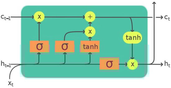
Figure 1.
The LSTM architecture [39].
The input gate, output gate, and forget gate are the three main mechanisms that regulate the flow of input and output information in the cell. The terms it, ot, and ft depicted in Figure 1 refer to the Ct and terms for the operational cell memory states of the network. The letter t, which appears as an index in all formulas, symbolizes the current time step of the relevant term [40].
Bidirectional Long Short-Term Memory (BiLSTM) is a sub-version of RNN architecture. This architecture processes as two independent RNN structures, enabling the networks to have both retrospective and prospective information about the sequence at each time frame. The BiLSTM system processes inputs in two ways, either backwards (from the future to the past) or forwards, which is the opposite [43,44].
3.3.3. RNN-Based Deep Learning (RNNBDL) Approach
Another motivation of the current study is to create a deep learning model potentially employed in software fault prediction with a synergistic approach using RNN type LSTM and BiLSTM deep neural network architectural models. The following neural network model was used in this context to predict software faults across three different data sets.
Table 1 displays the details of the RNN-based deep learning (RNNBDL) approach network model developed for software fault prediction. The developed model consists of five layers in total. The subjected neural network is expected to perform better when operating LSTM and BiLSTM layers in conjunction. In the created neural network, layer transitions are executed by reducing the total number of parameters by 50%. In the table, nIn represents the input size for the present layer, whereas nOut represents the number of hidden nodes for the present layer.

Table 1.
RNN-Based Deep Learning (RNNBDL) neural network model.
Hyper parameters are configuration options that describe how a DL model behaves. Parameter values are set before training without training the model for them. Examples of hyper parameters include the number of epochs, batch size, and learning rate. Adjusting these hyper parameters may significantly impact the performance of a machine learning model and finding optimal values for a given problem is typically a critical step in the model development procedure [45]. Several tests were conducted before the current study to determine the appropriate value range. The following details pertain to the selected hyper parameter. Epoch Counts: Since 1000 epochs produced the best results, this number was selected as an epoch value. Batch Size: This parameter specifies the number of samples that must be processed immediately before the parametric values of the model are updated, and 100 was chosen as the model value since it accounted for the best value in the study.
The ADAM (adaptive moments estimation) optimization method, analogous to the stochastic slope descent approach in the literature, was adopted to train neural networks [46,47]. An early stopping process was also employed while training the model. The initial value for the learning ratio started as 0.001 using the ‘Adam class.’ The total number of parameters and trainable parameters in the Active MQ Defect Data set model were 453.670 and 453.670, respectively. In Table 2, the parameter settings for the empirical results have been summarized.
Table 2.
The parameter settings for the empirical results.
3.4. Performance Evaluation Metrics
In the experimental results, classification models are evaluated with accuracy (ACC), area under curve (AUC), and Cohen’s kappa (KE) metrics. A confusion matrix is used to calculate several useful metrics like ACC and AUC. A confusion matrix created from a two-class classification problem can be seen in Table 3, in which four possible actual-to-estimated class mappings are represented by TP for true positive, FP for false positive, FN for false negative, and TN for true negative values.
Table 3.
A confusion matrix for a two-class problem.
ACC is a widely-used metric to determine the ability of the classifier for class distinction. It is defined as the percentage of the samples correctly classified by the algorithm [37]. ACC is calculated by the formula given in Equation (7).
The receiver operating characteristic (ROC) curve, or simply the ROC curve, enables a model to differentiate, facilitating the comparison of various models in terms of their effectiveness [37]. The most widely-used measurement is the area under curve (AUC) that remains under ROC curve. The performance of a classifier gets better as the AUC becomes larger. The possible values of AUC vary between 0.5 and 1.0. The AUC is calculated by the formula given in Equation (8).
Cohen’s kappa (KE) is a metric used to determine whether the performance of a classifier depends on chance. KE ranges between −1 and 1. As the KE value of the classifier approaches 1, the ACC value is deemed to be more realistic. KE is calculated by the formula given in Equation (6) [37]. In the Equation (9), po refers to “total agreement probability” and pc refers to “agreement probability” depending on chance.
Probability of detection (PD): As referred to by the term ‘Recall’, it is calculated by the ratios of negative values. Additionally, it is also calculated based on the division of the true negative value by the sum of the false negative and true negative values. The PD is calculated by the formula given in Equation (10).
Probability of false (PF): The computation process involves dividing the positive values by one another. It is calculated by dividing the false positive value by the sum of the true positive and false positive values. The PF is calculated by the formula given in Equation (11).
Precision (PR): Its calculation is based on dividing the true positive value by the sum of the true positive and false positive values. The PR is calculated by the formula given in Equation (12).
True negative rate (TNR): TNR is found by dividing the true negative value by the sum of the true negative and false positive values. The TNR is calculated by the formula given in Equation (13).
F-Measure (FM): The FM is employed to test the precision with the use of harmonic mean of precision and recall metrics, particularly those based on unbalanced data. Its calculation applies the following formula. The FM is calculated by the formula given in Equation (14).
4. New Experimental Data Set, Benchmark Data Sets and Software Measurement Data
In this research, a new data set named SFP XP-TDD comprised of several metrics of three separate software systems was created. The aforementioned three different software were developed as distinct domains of the same automation system, consisting of 472,443 lines of code for three software in total. Analysis, coding, testing, and maintenance phases of these software systems were continuously monitored in each iteration in accordance with the spiral software development methodology of XP. In accordance with TDD practice, the basic code was written first, followed by the functional code. The functional code was revised to be successful in the tests determined with TDD. These steps were repeated until all the tests were successful. New versions were created every three weeks using the continuous integration practice of XP. The testing of software systems in the data sets were considered separately in each phase starting from the analysis phase. In accordance with collective ownership practice of XP, it was subjected to the white-box unit testing method developed by the programmers and the team leader. In the final phase of the testing process, verification and acceptance testing was performed by the client with real production data. The delivery period of the software was completed with the receipt of approval being delivered by the client. A previously developed project management software was used actively throughout the process to keep track of all these steps. After the acceptance testing, faults observed in the software were recorded in the software project management tool in the maintenance phase. There was another separate software to track the errors of the software developed in the study. This software has logged errors that occurred during the six months following the use of the master versions of the developed software. Creation of ‘the Classes with Error section’ took place in the data set in this manner.
In this study, we have also used data sets from Eclipse and JIRA, and the Defect data set repository [48]. All bug prediction data sets were given in Table 1. By the nature of DL, it is necessary to use data with a sizable number of samples; thus, while selecting data sets, those data sets with numerous records were chosen rather than those comprising of a small number of samples. The first data set is from the Eclipse Equinox and Eclipse Core software project which were developed in the Java language system. The goal of the Equinox project is to be a first-class open service gateway initiative (OSGi) [48]. The second data set is form JIRA Defect prediction data set (Apache Active MQ) [49] which was developed using the Java language for the Java Message Service client infrastructure. In Table 4, general information about each project in the data sets are presented. The name of the last data set is SFP XP-TDD. This data set has been made publicly available for researchers to conduct their own studies and to have reproducible experimental results.
Table 4.
Description of SFP XP-TDD software metrics.
The SFP XP-TDD data set consists of 1,713 classes. There are approximately 300 code lines for each class in the data set. On average, 3.7% of each class consists of comments. The Table 4 below displays details about the metrics in the data set. The definition and description of these metrics are presented in Table 4.
In this study, we have also used datasets from Eclipse and JIRA. Eclipse and JIRA data sets are among the most-used datasets in the literature regarding software error estimation.
Defect dataset repository [48] and all bug prediction datasets are given in Table 5. By the nature of DL, it is necessary to use data with a sizable number of samples; as a result, datasets with numerous records were chosen above those comprising a small number of samples while selecting the dataset.
Table 5.
The general short descriptions of all data sets.
First dataset is from Eclipse Equinox and Eclipse Core software project which were developed in the Java language system. The goal of the Equinox project is to be a first-class open service gateway initiative (OSGi) [48]. The second dataset is from the JIRA Defect prediction dataset (Apache Active MQ) [49] which was developed in Java language for the Java Message Service client infrastructure. In Table 5, general information about each project in the datasets are presented. The last dataset’s name is SFP XP-TDD. This dataset has been made publicly available for researchers to conduct their own studies and to have reproducible experimental results.
The Eclipse data set, the minimum data set in terms of the number of modules in the study, consists of 37 measurements. This data set includes Chidamber and Kemer (CK) metrics, Object-Oriented (OO) metrics, and entropy metrics. However, the last domain module in the data set refers to the ‘bug’ domain, which detects whether the module is faulty [9,49]. The Apache Active MQ refers to the most comprehensive data set in the study, consisting of 3420 modules and 66 software metrics. Chidamber and Kemer (CK), object-oriented (OO) [9,50] entropy, and exchange metrics were all applied to this data set. The ‘Heubug’, which indicates whether the module is faulty, was the latest domain in the data set. The final data set, the SFP XP-TDD, is the second most ample data set within the context of the number of modules. It consisted of 1713 modules and 14 software metrics, comprising of Object-Oriented (OO) entropy and exchange metrics. Similarly, ‘Error’ is the last domain in this data set, detecting whether or not the module is faulty.
The three data sets were all created for software fault predictions, and each data set retained a variety of metrics that are unique to that data set. The general metrics type information of all datasets are presented in Table 6.
Table 6.
The general metrics type information of all data sets.
5. Experimental Results and Discussion
In this section, the methodology, the experimental results, and the evaluations of the results are presented.
5.1. Methodology
This section covered the methodology followed in the study in five consecutive steps. The initial step studied the data sets listed in the 4th section, while the second step focused on the training procedures of these data sets with the 10-fold cross-validation method.
The third step involved examining three subgroups of algorithms within itself. The initial part of the third step discussed five separate conventional machine learning algorithms displayed in Figure 2, in addition to addressing the versions of these algorithms using Rotation Forest ensemble models. The second part of the third step concentrated on deep learning algorithms such as CNN, LSTM, and BiLSTM. The final part of the third step, on the other hand, discussed the RNN-based deep learning approach (RNNBDL) algorithm. These chosen algorithms were tested in the fourth step using the 10-fold cross-validation method. Finally, the fifth step summarized the performances, statistical outcomes, values, and evaluation metrics acquired from the tests run. The pipeline of the workflow and its complete architecture are given in Figure 2. This section covered the methodology followed in the study in five consecutive steps. The initial step studied the data sets listed in the 4th section, while the second step focused on the training procedures of these datasets with the 10-fold cross-validation method. In Algorithm 1, the main stages of the workflow and its complete architecture have been briefly summarized.
| Algorithm 1. Pseudo-code of the proposed scheme. |
| //Step 1: Input & Output //Input DataSets[]:array [Eclipse,SFP-XP-TDD, Active MQ]; MLAlg []: array [KNN,NB,RT,KSTAR,SVM]; eMLAlg []: array [eKNN,eNB,eRT,eKSTAR,eSVM]; DLAlg []: array [CNN,LSTM,BiLSTM,RNNBDL]; int location = 0; //TFCC meaning Ten Fold Cross Validation //Output MLResults_ACC[]: array; eMLResults_ACC[]: array; DLResults_ACC[]: array; //Step 2: Training MLTrainResults[]:array [TFCV(MLAlg[DataSets])]; eMLTrainResults[]:array[TFCV(EnsMLAlg[DataSets])]; DLTrainResults: array [TFCV(DLearningAlg[DataSets])]; //Step 3 & 4: Execute the Method & Test while (location < DataSets[].length) { for (i = 0;i < MLAlg.length;i++) { MLResults_ACC [] = Test(MLTrainResults[]); eMLResults_ACC[] = Test(eMLTrainResults[]); } for (i = 0;i < DLAlg.length;i++) { DLResults_ACC [] = Test(DLTrainResults[]); } location++; } //Step 5: Evaluation Metrics location = 0; while (location < DataSets[].length) { printf(“Machine Learing ACC Results”); for (i = 0;i < MLAlg.length;i++){ printf(MLResults_ACC[i];} printf(“Ensemble Machine Learning ACC Results”); for (i = 0;i < eMLAlg.length;i++){ printf(eMLResults_ACC[i];} printf(“Deep Learing ACC Results”); for (i = 0;i < DLAlg.length;i++){ printf(DLResults_ACC[i];} } |
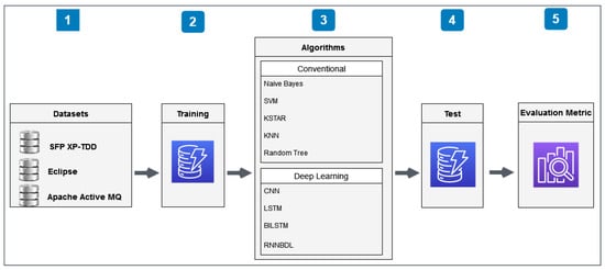
Figure 2.
The pipeline of the workflow and its complete architecture.
SVM, KNN, NB, and CNN are non-sequential models frequently used in tasks such as classification and regression. The input data for these tasks does not retain a temporal dimension. While LSTM- and RNN-based sequential models are designed for sequential datasets such as time series or natural language, they are potentially utilized for classification in datasets without time series[51]. Besides, using non-sequential and sequential models together might enable each model to display its own power. In such systems, a non-sequential model may serve as a feature extractor, and then the extracted features may be utilized as input to a sequential model. However, the current study achieved performances on ACC and FM-based metrics separately using the SFP datasets with no temporal dimension on sequential and non-sequential models.
5.2. Conventional Machine Learning Experimental Results
The SFP XP-TDD data set, the Eclipse data set and the Apache Active MQ Defect data set’s experimental results of the classification algorithms are presented in Table 7, Table 8 and Table 9. In these tables, the word ‘Algorithm’ refers to the machine learning algorithm names in column 1. ACC, AUC, FM, and KE are the metrics obtained by running through the respective algorithms. eACC, eAUC, eFM, and eKE are, on the other hand, the ones obtained by running through the Rotation Forest ensemble classifier generated by using the respective algorithms as the base classifiers. Diff is the difference between ACC and eACC. As seen in Table 7, the highest value in each column is marked through bolding and shading.
Table 7.
Classification results for SFP XP-TDD data set.
Table 8.
Classification results for Eclipse data set.
Table 9.
Classification results for Active MQ data set.
5.2.1. SFP XP-TDD Data Set Experimental Results
According to the experiments, no significant increase or decrease was seen in the Naive Bayes and KSTAR algorithms. ACC values of the remaining algorithms has shown an increase. As seen in Table 3, the average eACC value of the five base classifiers is 94.30%, and the average ACC is 93.61%. The Diff value that shows the difference between two primary metrics indicates a positive increase of 0.69%. Similarly, the average AUC increased from 0.772 to 0.825 and the average FM increased from 0.929 to 0.936.
Table 7 clearly shows that the SVM classifier and Random Tree ensembles classifiers have a higher ACC compared to the other classifiers. They have a better ACC value in 94.92% of the five algorithms in question.
5.2.2. Eclipse Data Set Experimental Results
The Eclipse data set experimental results of the classification algorithms are presented in Table 8. According to the experiments, no significant increase or decrease was seen in the Naive Bayes algorithms. ACC values of the remaining algorithms increased. As seen in Table 8, the average eACC value of five base classifiers is 70.74%, and the average ACC is 76.54%. The Diff value that shows the difference between two primary metrics indicates a positive increase of 5.80%. Similarly, the average AUC increased from 0.701 to 0.815 and the average FM increased from 0.727 to 0.761.
Table 8 clearly shows that SVM ensembles classifier has a higher ACC compared to the other classifiers. It has a better ACC in 79.93% among five algorithms.
5.2.3. Active MQ Defect Data Set Experimental Results
The Active MQ Defect Data experimental results of the classification algorithms are presented in Table 9. According to the experiments, no significant increase or decrease was seen in the SVM algorithm.
On the other hand, ACC values of the algorithm Naive Bayes had reduced. However, ACC values of the remaining algorithms had increased. As seen in Table 6, the average eACC value of the five base classifiers is 91.93% and the average ACC is 91.80%. The Diff value that shows the difference between two primary metrics indicates a negative difference of 0.13%. This result can be attributed to the results of Naive Bayes’ classification. Similarly, the average FM decreased. Nevertheless, AUC demonstrated a very small increase, from 0.910 to 0.913.
The choice of the algorithm may vary based on several factors, such as the data type, problem complexity, and the desired level of accuracy. For instance, if the problem is a straightforward classification task with a modest amount of clean and structured data, algorithms such as ‘KNN’ or logistic regression may be satisfactory. Therefore, it might be reasonable to test various machine learning algorithms and compare their performance on the same problem to solve the problem and resolve which approach will perform better.
Table 9 clearly shows that the Random Tree ensembles classifier has a higher ACC compared to the other classifiers. It has a better ACC in 94.38% among the five algorithms. The support vector machines (SVM) algorithm is a machine learning approach that generates quite successful outcomes, especially in multidimensional data sets. This algorithm aims to determine the most suitable plane (support vector) to classify the data points into two groups. The SVM algorithm potentially achieves more successful outcomes if the relationships between the properties are powerful. However, the Random Tree algorithm is a decision tree algorithm based on property values. This algorithm is also known for achieving a high performance with large data sets. The ensemble RF combines the predictions of multiple models to create a final prediction. It can create final predictions robustly and accurately by using multi-models. Thus, the errors made by individual models may be compensated for by other models in the ensemble, leading to a more accurate overall prediction. Therefore, using the ensemble Rotation Forest with precise and robust algorithms like SVM and Random Tree can further improve the accuracy and robustness of the final prediction.
5.3. Deep Learning Experimental Results
Table 10 displays the experimental outcomes of the deep learning algorithms on the SFP XP-TDD data set, Eclipse Equinox data set, and Apache Active MQ Defect data set. The first column in the table lists the data set names. The term algorithm refers to the deep learning algorithm names in column 2. The metrics derived by running with the respective algorithms are ACC, AUC, FM, and KE. As depicted in Table 6, despite the outcomes obtained from deep learning algorithms with the first data set, the SFP XP-TDD were highly similar to one another; all the acquired results generated a higher classification performance rate than those of machine learning algorithms. Furthermore, the deep learning algorithm results not only outperformed all machine learning algorithm outcomes, but those outcomes were also higher than other ensemble classifier results of machine learning in terms of performance rate.
Table 10.
Deep Learning Algorithm Based Classification results for All Data set.
The review of the Eclipse Equinox data illustrated in the second row in Table 10 indicates that the BiLSTM algorithm achieved a better performance than other algorithms, whereas this performance rate was lower than the ensemble classifier result of the SVM algorithm. However, the average deep learning algorithms’ ACC success rate of 77.77% was explicitly higher than the average ACC performance rates for machine learning ensemble classifiers and base classifiers, which are both 70.64% and 76.54%, respectively.
The performance rates of all algorithms posed comparable values to one another, according to the analysis of the Active MQ results displayed in Table 10’s last row. In addition to having higher performance rates than all other machine learning algorithms, the outcomes of deep learning algorithms also exceeded the performance rates of all machine learning ensemble classifiers.
There are fewer types of metrics available in the SFP-XPTDD and Eclipse data sets. However, The ActiveMQ data set comprises numerous metrics comprising unique patterns for more categories. Therefore, it seems that the LSTM and BiLSTM algorithm in the SFP-XPTDD and Eclipse data sets and the CNN algorithm, processing the discrete sections more effectively in the ActiveMQ data set, result in better outcomes.
RNN Based Deep Learning (RNNBDL) Experimental Results
Table 11 lists the results of the RNNBDL algorithm for the three separate data sets used in the study. As depicted in the results, the SFP XP-TDD, the initially employed data set, yielded higher values than those of other machine learning algorithms; however, they also attained the same value as the LSTM results, which is a deep learning algorithm. Analysis of the data related to the Eclipse, the second data set in the study, also revealed that the ACC ratio of 78.46%, achieved from the RNNBDL algorithm, was below the Rotation Forest ensemble classifier ratio of the SVM algorithm, which is a machine learning algorithm. Similarly, it lagged behind BiLSTM, a deep learning algorithm, despite the fact that the value obtained by the RNNBDL algorithm was higher than the average values acquired with both machine learning and deep learning algorithms. When comparing the results of tests performed on the Active MQ data set, the RNNBDL data was slightly higher than those acquired in both machine learning and deep learning algorithms. The RNNBDL algorithm, on the other hand, is thought to provide better outcomes on selected data sets with large sample sizes since it is a deep learning-based algorithm, and thus it is capable of making high-level interpretations with DL and being a semantically-enriched feature extraction.
Table 11.
RNNBDL Algorithm Based Classification results for All Data set.
5.4. Discussion of Results
Table 12 compares the outcomes of the RNNBDL algorithm with those of other algorithms. An experimental study assessed the distinction between using five selected machine learning algorithms over three separate data sets and the Rotation Forest ensemble of these five different machine learning algorithms. Analysis of ten different results revealed that the Rotation Forest ensemble boosted the performance rate in all other results except the Naive Bayes algorithm. In addition to machine learning algorithms for software bug prediction, they were employed in deep learning algorithms to perform additional tests. The acquired results indicate that deep learning algorithms potentially detect extremely faulty modules with high accuracy. The final step of the study focused on developing an algorithm named RNNBDL and applied this algorithm to three separate data sets. Although the results of the RNNBDL algorithm were not promising, these results are still higher than the averages of the deep learning and machine learning algorithms. Figure 3 shows the success rates of ACC based average increments between base classifiers and ensemble classifiers. Figure 4 shows the success rates of the ACC-based average increments between DL and ML.
Table 12.
Overall Evaluation of Experimental Results based on ACC.
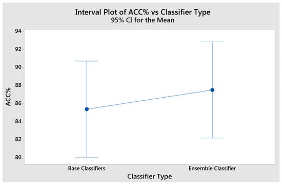
Figure 3.
ACC-based average increments between base classifiers and ensemble classifiers.
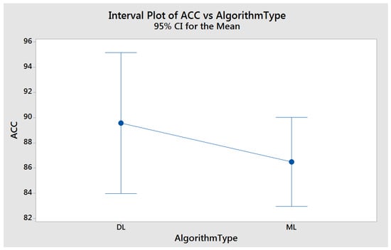
Figure 4.
ACC based average increments between DL and ML.
Finally, the study developed an algorithm named RNNBDL and applied it to three separate data sets. Table 12 compares the ACC results from the RNNBDL deep learning algorithm with the ACC findings from all other tests. As depicted in Table 12, the RNNBDL algorithm outperformed other algorithms in terms of performance.
Figure 5 illustrates the main effects plot for accuracy based on the methods and data sets. As depicted in Figure 5, the suggested algorithm, RNNDBL, achieved the highest average classification accuracy. However, the SVM base classifier algorithm generated the lowest average classification accuracy. Further details of the experimental results of DL and ML are presented in Figure 5.
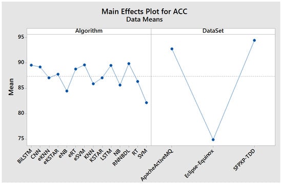
Figure 5.
The main effects plot for accuracy based on the methods and the main effects plot for accuracy based on the data sets.
6. Test and Validation
ANOVA is a test used to decide whether there is a semantic difference between more than two independent groups. Hence, the ANOVA test, also denoted as the analysis of variance, was performed to examine the statistical significance of the data acquired to verify the results produced by the independent values. The n-way ANOVA test was employed to determine the statistical validity of applying deep learning algorithms in place of machine learning algorithms in the statistical test since the variable value was more than one [52].
In the study carried out for data sets with large record numbers as illustrated in Table 13, a p-Value of 0.008, which is a much smaller value than 0.05, indicates that running tests with DL algorithms with 95% confidence displayed a statistically higher performance than ML algorithms.
Table 13.
Overall Evaluation of Experimental Results based on ACC.
7. Threads to Validity
A novel data set, SFP XP-TDD, was tested as part of the comparison of several techniques in the study for software fault predictions, while at the same time, Eclipse and Active MQ, two other data sets with a history in the literature, were utilized to benchmark the results. As a result, the study primarily led to three conclusions.
The first conclusion is that almost all outcomes perform better when the Rotation Forest ensemble is used, which escalates the performance rate of machine learning algorithms. The second conclusion is the successful use of deep learning algorithms in software fault predictions. Finally, the third conclusion is the achievement of successful outcomes when utilizing an RNN-based deep learning model with many layers to predict faults. Numerous studies in the literature reported the detailed SFP performance of ML algorithms. These publications also revealed that even the NASA KC1-like software fault prediction data sets comprised approximately 300–400 samples. However, the current study, expressly demonstrating the performance of software fault prediction of DL algorithms, employed a sizable data set with at least 1000 samples, resulting in marginally above the performance rate of ML algorithms. If data sets with sizable sample numbers are created and used, it is explicit that the performance rate of DL algorithms will be much higher than ML algorithms. However, reviewing the currently issued articles indicated that it was impossible to use such sizable software fault prediction data sets since they did not exist in the literature.
8. Conclusions and Future Work
In this study, three different software projects with more than 472,000 lines of code were developed by a seven-person development team by adhering largely to the life cycle and the work environment of XP and by practicing TDD. A project management tool was also developed to help manage the projects effectively by keeping track of the development progress and status of the observed faults. Then, a data set named SFP XP-TDD was created using the software metrics data of these software in order to conduct software with 547,546 fault prediction research, which was then used in the study for data sets with large record numbers.
The experimental results of the study were also used to benchmark against data sets from Apache Active MQ and Eclipse. Machine learning models were trained and tested using the data set to perform software fault prediction. Experiments were performed on the data set with five different base classifiers and the RF ensembles of these classifiers. The experimental results demonstrate that higher accuracy rates were achieved with the ensemble RFs when compared to their respective base classifiers. Increases were observed not only in ACC values, but also in KE and AUC values. Considering the general averages, the value of ACC was observed to be increased by 2.12%. Furthermore, a rise in the averages of AUC and KE values support the performance increase in classifiers. In addition to the average performance values, an increase was observed in all three metrics with RF ensembles of 10 of 15 algorithms seen in Table 3, Table 4 and Table 5.
This study used OO metrics, entropy metrics, and change metrics, in addition to CK metrics on the data sets to conduct experiments and test the performance rates of algorithms. Besides utilizing ML algorithm-based software fault prediction, the current study also used several other software fault predictions alongside DL algorithms that achieved significant success in many diverse fields, including computer vision, natural language processing, and speech recognition. Finally, to conduct software fault prediction with deep learning methods, this study made a software fault prediction using a DL neural network called RNNBDL, comprised of LSTM and BILSTM algorithms, in addition to a combination of CNN, LSTM, and BiLSTM.
In the study carried out for data sets with large record numbers, it was also concluded that successful outcomes were achieved when an RNN-based deep-learning model with many layers was utilized in fault prediction. The n-way ANOVA statistical method compared both the results of machine learning and deep learning algorithms. Accordingly, the test results concluded that it is possible to prefer using deep learning algorithms instead of machine learning algorithms in studies performed with a 95% confidence rate for large software fault data sets. It is viable to employ the resulting data set in cross-project defect prediction. The subsequently designed studies will focus on generating a new data set using Java Doc documents, aiming to incorporate transfer learning into the novel work developed with a brand new hybrid technology.
Funding
This research received no external funding.
Institutional Review Board Statement
Not applicable.
Informed Consent Statement
Not applicable.
Data Availability Statement
Not applicable.
Conflicts of Interest
The authors declare no conflict of interest.
References
- Hughes, B.; Cotterell, M. Software Project Management, 5th ed.; McGraw-Hill Education: New York, NY, USA, 2009. [Google Scholar]
- Çatal, Ç. Software Engineering Methods-Advanced Topics; Papatya Publishing: Istanbul, Türkiye, 2012. [Google Scholar]
- Schach, S.R. Object-Oriented and Classical Software Engineering; McGraw-Hill: New York, NY, USA, 2011. [Google Scholar]
- McGregor, J.D.; Sykes, D.A. A Practical Guide to Testing Object-Oriented Software; Addison-Wesley Longman Publishing Co., Inc.: Boston, MA, USA, 2001. [Google Scholar]
- Juneja, K. A fuzzy-filtered neuro-fuzzy framework for software fault prediction for inter-version and inter-project evaluation. Appl. Soft Comput. J. 2019, 77, 696–713. [Google Scholar] [CrossRef]
- Batool, I.; Khan, T.A. Software fault prediction using data mining, machine learning and deep learning techniques: A systematic literature review. Comput. Electr. Eng. 2022, 100, 107886. [Google Scholar] [CrossRef]
- Schwaber, K.; Beedle, M. Agile Software Development with Scrum, 1st ed.; Pearson: New York, NY, USA, 2001. [Google Scholar]
- Gerald, D.E.; Raymond, M., Jr. Software Testing Across the Entire Software Development Life Cycle; Wiley-IEEE Computer: Hoboken, NJ, USA, 2007. [Google Scholar]
- Succi, G.; Pedrycz, W.; Djokic, S.; Zuliani, P.; Russo, B. An Empirical Exploration of the Distributions of the Chidamber and Kemerer Object-Oriented Metrics Suite. Empir. Softw. Eng. 2005, 10, 81–104. [Google Scholar] [CrossRef]
- Mauša, G.; Grbac, T.G.; Bašić, B.D. A Systematic Data Collection Procedure for SoftwareDefect Prediction. Comput. Sci. Inf. Syst. 2016, 13, 173–197. [Google Scholar] [CrossRef]
- Apache Active MQ Bug Prediction Data Set; The Apache Software Foundation: Wilmington, Delaware, USA, 2022; Available online: https://downloads.apache.org/ (accessed on 15 May 2022).
- Akman, M.; Genç, Y.; Ankaralı, H. Random Forests Methods and an Application in Health Science. Turk. Klin. J. Biostat. 2011, 3, 36–48. [Google Scholar]
- Ostrand, T.J.; Weyuker, E.J.; Bell, R.M. Predicting the Location and Number of Faults in Large Software Systems. IEEE Trans. Softw. Eng. 2005, 31, 340–355. [Google Scholar] [CrossRef]
- Turhan, B.; Bener, A. A Multivariate Analysis of Static Code Attributes for Defect Prediction. In Proceedings of the 7th International Conference on Quality Software QSIC 2007, Portland, OR, USA, 11–12 October 2007; pp. 231–237. [Google Scholar]
- Song, Q.; Shepperd, M.; Cartwright, M.; Mair, C. Software Defect Association Mining and Defect Correction Effort Prediction. IEEE Trans. Softw. Eng. 2006, 32, 69–82. [Google Scholar] [CrossRef]
- Weyuker, E.J.; Ostrand, T.J.; Bell, R.M. Adapting a Fault Prediction Model to Allow Widespread Usage. In Proceedings of the 4th International Workshop on Predictive Models in Software Engineering, Leipzig, Germany, 12–13 May 2008. [Google Scholar]
- Çatal, Ç.; Sevim, U.; Diri, B. Software Fault Prediction of Unlabeled Program Modules. In Proceedings of the World Congress on Engineering 2009, London, UK, 1–3 July 2009; pp. 212–217. [Google Scholar]
- Çatal, Ç.; Diri, B. Investigating the Effect of Data set Size, Metrics Sets, and Feature Selection Techniques on Software Fault Prediction Problem. Inf. Sci. 2009, 179, 1040–1058. [Google Scholar] [CrossRef]
- Weyuker, E.J.; Ostrand, T.J.; Bell, R.M. Do Too Many Cooks Spoil the Broth? Using the Number of Developers to Enhance Defect Prediction Models. Empir. Softw. Eng. 2008, 13, 539–559. [Google Scholar] [CrossRef]
- Menzies, T.; Greenwald, J.; Frank, A. Data Mining Static Code Attributes to Learn Defect Predictors. IEEE Trans. Softw. Eng. 2007, 33, 2–13. [Google Scholar] [CrossRef]
- Zhou, Y.; Leung, H. Empirical Analysis of Object-Oriented Design Metrics for Predicting High and Low Severity Faults. IEEE Trans. Softw. Eng. 2006, 32, 771–789. [Google Scholar] [CrossRef]
- Çatal, Ç. Software Fault Prediction: A Literature Review and Current Trends. Expert Syst. Appl. 2011, 38, 4626–4636. [Google Scholar] [CrossRef]
- Arisholm, E.; Briand, L.C.; Johannessen, E.B. A Systematic and Comprehensive Investigation of Methods to Build and Evaluate Fault Prediction Models. J. Syst. Softw. 2010, 83, 2–17. [Google Scholar] [CrossRef]
- Jin, C.; Jin, S.-W. Prediction Approach of Software Fault-proneness Based on Hybrid Artificial Neural Network and Quantum Particle Swarm Optimization. Appl. Soft Comput. 2015, 35, 717–725. [Google Scholar] [CrossRef]
- Manjula, C.; Florence, L. Deep neural network based hybrid approach for software defect prediction using software metrics. Clust. Comput. 2019, 22, 9847–9863. [Google Scholar] [CrossRef]
- Lino Ferreira da Silva Barros, M.H.; Oliveira Alves, G.; Morais Florêncio Souza, L.; da Silva Rocha, E.; Lorenzato de Oliveira, J.F.; Lynn, T.; Sampaio, V.; Endo, P.T. Benchmarking Machine Learning Models to Assist in the Prognosis of Tuberculosis. Informatics 2021, 8, 27. [Google Scholar] [CrossRef]
- Yucalar, F.; Ozcift, A.; Borandag, E.; Kilinc, D. Multiple-classifiers in software quality engineering: Combining predictors to improve software fault prediction ability. Eng. Sci. Technol. Int. J. 2020, 23, 938–950. [Google Scholar] [CrossRef]
- Qiao, L.; Li, X.; Umer, Q.; Guo, P. Deep learning based software defect prediction. Neurocomputing 2020, 385, 100–110. [Google Scholar] [CrossRef]
- Abdu, A.; Zhai, Z.; Algabri, R.; Abdo, H.A.; Hamad, K.; Al-antari, M.A. Deep Learning-Based Software Defect Prediction via Semantic Key Features of Source Code—Systematic Survey. Mathematics 2022, 10, 3120. [Google Scholar] [CrossRef]
- Brownlee, J. What is Deep Learning? Machine Learning Mastery. 16 August 2019. Available online: https://machinelearningmastery.com/what-is-deep-learning/ (accessed on 20 October 2022).
- Borandag, E.; Ozcift, A.; Kilinc, D.; Yucalar, F. Majority vote feature selection algorithm in software fault prediction. Comput. Sci. Inf. Syst. 2019, 16, 515–539. [Google Scholar] [CrossRef]
- Alpaydin, E. Introduction to Machine Learning, 2nd ed.; The MIT Press: Cambridge, MA, USA, 2010. [Google Scholar]
- Breiman, L. Bagging Predictors. Mach. Learn. 1996, 24, 123–140. [Google Scholar] [CrossRef]
- Schapire, R.E. A Brief Introduction to Boosting. In Proceedings of the 16th International Joint Conference on Artificial Intelligence IJCAI 1999, Stockholm, Sweden, 31 July–6 August 1999; pp. 1401–1406. [Google Scholar]
- Breiman, L. Random Forests. Mach. Learn. 2001, 45, 5–32. [Google Scholar] [CrossRef]
- Rodriguez, J.J.; Kuncheva, L.I.; Alonso, C.J. Rotation Forest: A New Classifier Ensemble Method. IEEE Trans. Pattern Anal. Mach. Intell. 2006, 28, 1619–1630. [Google Scholar] [CrossRef]
- Ozcift, A.; Gulten, A. Classifier Ensemble Construction with Rotation Forest to Improve Medical Diagnosis Performance of Machine Learning Algorithms. Comput. Methods Programs Biomed. 2011, 104, 443–451. [Google Scholar] [CrossRef]
- Bengio, Y.; LeCun, Y.; Hinton, G. Deep Learning. Nature 2015, 521, 436–444. [Google Scholar]
- Gündüz, G.; Cedimoğlu, İ.H. Gender Prediction from Image Using Deep Learning Algorithms. Sak. Univ. J. Comput. Inf. Sci. 2019, 2, 9–17. [Google Scholar]
- Rojas-barahona, L.M. Deep learning for sentiment analysis. Lang. Linguist. Compass 2016, 10, 701–719. [Google Scholar] [CrossRef]
- Pant, D.R.; Neupane, P.; Poudel, A.; Pokhrel, A.; Lama, B.K. Recurrent neural network based Bitcoin price prediction by Twitter sentiment analysis. In Proceedings of the IEEE 3rd International Conference on Computing, Communication and Security, Kathmandu, Nepal, 25–27 October 2018; pp. 128–132. [Google Scholar]
- Liu, G.; Guo, J. Bidirectional LSTM with attention mechanism and convolutional layer for text classification. Neurocomputing 2019, 337, 325–338. [Google Scholar] [CrossRef]
- Schmidhuber, J. Deep learning in neural networks: An overview. Neural Netw. 2015, 61, 85–117. [Google Scholar]
- Fan, G.; Diao, X.; Yu, H.; Yang, K.; Chen, L. Software defect prediction via attention-based recurrent neural network. ScientificProgramming 2019, 2019, 6230953. [Google Scholar] [CrossRef]
- Ali, A.; Gravino, C. An empirical comparison of validation methods for software prediction models. J. Softw. Evol. Process 2021, 33, e2367. [Google Scholar] [CrossRef]
- Chollet, F. Deep Learning with Python; Manning Publications: Shelter Island, NY, USA, 2017. [Google Scholar]
- Kingma, D.P.; Ba, J. Adam: A Method for Stochastic Optimization, ICLR 2015. arXiv 2014, arXiv:1412.6980. [Google Scholar] [CrossRef]
- Eclipse Bug Prediction Data Set; The Eclipse Foundation: Ottawa, Canada; Available online: https://www.eclipse.org/org/foundation/January2022. (accessed on 15 May 2022).
- Flexible & Powerful Open Source Multi-Protocol Messaging. Apache Active MQ. 2022. Available online: https://activemq.apache.org/ (accessed on 20 October 2022).
- Tutorial on McCabe and Halsted. 2018. Available online: http://openscience.us/repo/defect/mccabehalsted/tut.htm (accessed on 20 October 2022).
- Wei, H.; Hu, C.; Chen, S.; Xue, Y.; Zhang, Q. Establishing a software defect prediction model via effective dimension reduction. Inf. Sci. 2019, 477, 399–409. [Google Scholar] [CrossRef]
- Borandağ, E.; Özçift, A.; Kaygusuz, Y. Development of majority vote ensemble feature selection algorithm augmented with rank allocation to enhance Turkish text categorization. Turk. J. Electr. Eng. Comput. Sci. 2021, 29, 514–530. [Google Scholar] [CrossRef]
Disclaimer/Publisher’s Note: The statements, opinions and data contained in all publications are solely those of the individual author(s) and contributor(s) and not of MDPI and/or the editor(s). MDPI and/or the editor(s) disclaim responsibility for any injury to people or property resulting from any ideas, methods, instructions or products referred to in the content. |
© 2023 by the author. Licensee MDPI, Basel, Switzerland. This article is an open access article distributed under the terms and conditions of the Creative Commons Attribution (CC BY) license (https://creativecommons.org/licenses/by/4.0/).