Article

Soil Depth Prediction Model Using Terrain Attributes in Gangwon-do, South Korea

Department of Civil & Environmental Engineering, University of Ulsan, Ulsan 44610, Republic of Korea
*
Author to whom correspondence should be addressed.
Appl. Sci. 2023, 13(3), 1453; https://doi.org/10.3390/app13031453
Submission received: 10 November 2022 / Revised: 27 December 2022 / Accepted: 29 December 2022 / Published: 22 January 2023
(This article belongs to the Special Issue Advances in Remote Sensing and GIS for Natural Hazards Assessment)

Abstract

:
Soil depth is a crucial parameter in slope stability analysis in mountainous areas. The drilling survey is the most reliable method for determining soil depth, but it requires a high cost for the vast geographical area. Therefore, this study proposes a soil depth prediction model for mountainous areas that uses Terrain Attributes (TAs) from digital maps. Gangwon-Do, a predominantly mountainous region in South Korea, is selected as the study target area. The study area is classified by parent rock type into igneous rocks, metamorphic rocks, and sedimentary rocks. The correlation with TAs is analyzed through multi-collinearity using drilling data published in the Korea drilling information database. In addition, the most suitable combination of variables is selected through multi-collinearity analysis, and the regression model using STI, TWI, and SLOPE is found to be the most appropriate model (VIF < 10). The proposed model for soil depth shows significance at p < 0.001, and the correlation coefficient ( R 2 ) is figured out for igneous rock (0.702), metamorphic rock (0.686), and sedimentary rock (0.693). In addition, the reliability of the proposed model was verified by using data from regions not included in the model development, and the correlation coefficients were igneous rock (0.867), metamorphic rock (0.801), and sedimentary rock (0.814). The model proposed is more suitable for Korean topography than the existing statistical models; it can help to increase the accuracy of slope stability analysis.

1. Introduction

Soil depth is defined as the vertical distance from the ground surface to bedrock [1,2,3,4]. The soil depth can be changed by erosion and weathering, and it is determined by various environmental variables, including slope, land use, curvature, parent material, weathering rate, climate, vegetation cover, upslope contributing area, and lithology [5,6]. In addition, the weathering depth varies depending on the rock type [7], and the distribution of soil depth will be different accordingly.
Soil depth plays an important role in landslide disaster prevention and management. The increasingly complex shallow landslide generation process integrates with physically based models such as SHALSTAB [8], SHETRAN [9], GEOtop FS+ [10], TRIGRS [11], and H-slider [12] to predict spatial patterns of landslide occurrences [12,13,14,15]. However, most of the analysis methods using landslide analysis models are carried out under the assumption that the soil depth is constant without consideration of the spatial distribution for soil depth [8,12,13,16,17,18]. Additionally, the flow of groundwater and the formation of wetting front, which have a significant effect on the stability of the slope, are also significantly affected by the soil depth and its spatial distribution [19,20].
Many researchers have conducted studies on how to predict soil depth, and these studies can be classified broadly into three groups: (1) physically based, (2) interpolation-based, and (3) regression methods.
The physically based model for soil depth prediction was developed as a landscape evolution model to solve the soil mass-balance equation over time [5]. Most landscape evolution models use linear sediment transport laws, which assume that the terrain slope and the sediment amount are equal. Although it develops into a simple analytical solution for mass balance, observational results report that landslides contribute to soil transport [5,21,22,23,24]. Recently, non-linear transport laws have been used to predict slope failure [23,25,26] and to describe the planar topography of steep slopes [27].
Interpolation-based soil depth prediction methods include IDW [28], Kriging [29,30], Co-Kriging [31], regression-kriging, and so on [3,32]. These days, many researchers have suggested the interpolation method to predict the spatial distribution of the soil depth, and this method often shows high accuracy compared to other methods. Penížek and Borůvka [33] reported that the co-kriging method showed higher accuracy than the ordinary kriging (OK), regression kriging (RK), and linear regression methods. However, although the interpolation method is convenient to use, it requires a large amount of data [5,34,35], and it cannot be said to show high accuracy in all cases because the deviation is significant due to the various environmental variables [36].
Regression methods correlate soil depth with TAs from digital elevation maps (DEMs) [33,37,38,39]. Goodman [40] reported that the coefficient of determination ( R 2 ) of the slope angle, absolute height, and relative height with soil depth were 0.46, 0.36, and 0.37, respectively. Gessler et al. [41] also analyzed the statistical correlation between soil depth and plan curvature, compound topographic index, and upslope mean plan curvature. Additionally, Qiyoung et al. [4] suggested that the correlation coefficient between the regression model using slope and TWI as variables and soil depth was 64.1%, and Mehnatkesh et al. [2] reported that the correlation coefficient between slope, wetting index, catchment area, and STI with soil depth was 76%.
In this paper, the study area was classified into igneous rock, metamorphic rock, and sedimentary rock, which are representative rock type in Korea. The correlation between TAs and soil depth in the study area is analyzed. Additionally, Using the multiple linear regression method, we propose a soil depth prediction model for each rock type that is suitable for the geological condition in Korea.

2. Methodology

2.1. Study Area and Terrain Attributes

The study area is selected as Gangwon-do in South Korea (Figure 1), with a total area of 16,827.93 km2 and a population of 1,539,521 (population density of 90 people/km2). Gangwon-do has the most mountainous region and the lowest population density in Korea [42]. To estimate the terrain attributes of the study area, a digital map (scale 1:25,000) of data from the National Geographic Information Institute [43] is used. Terrain attributes are derived using ESRI’s ArcGIS (ArcMap 10.1). Definitions and results of each derived terrain attribute are shown in Table 1.

2.2. Statistics Analysis

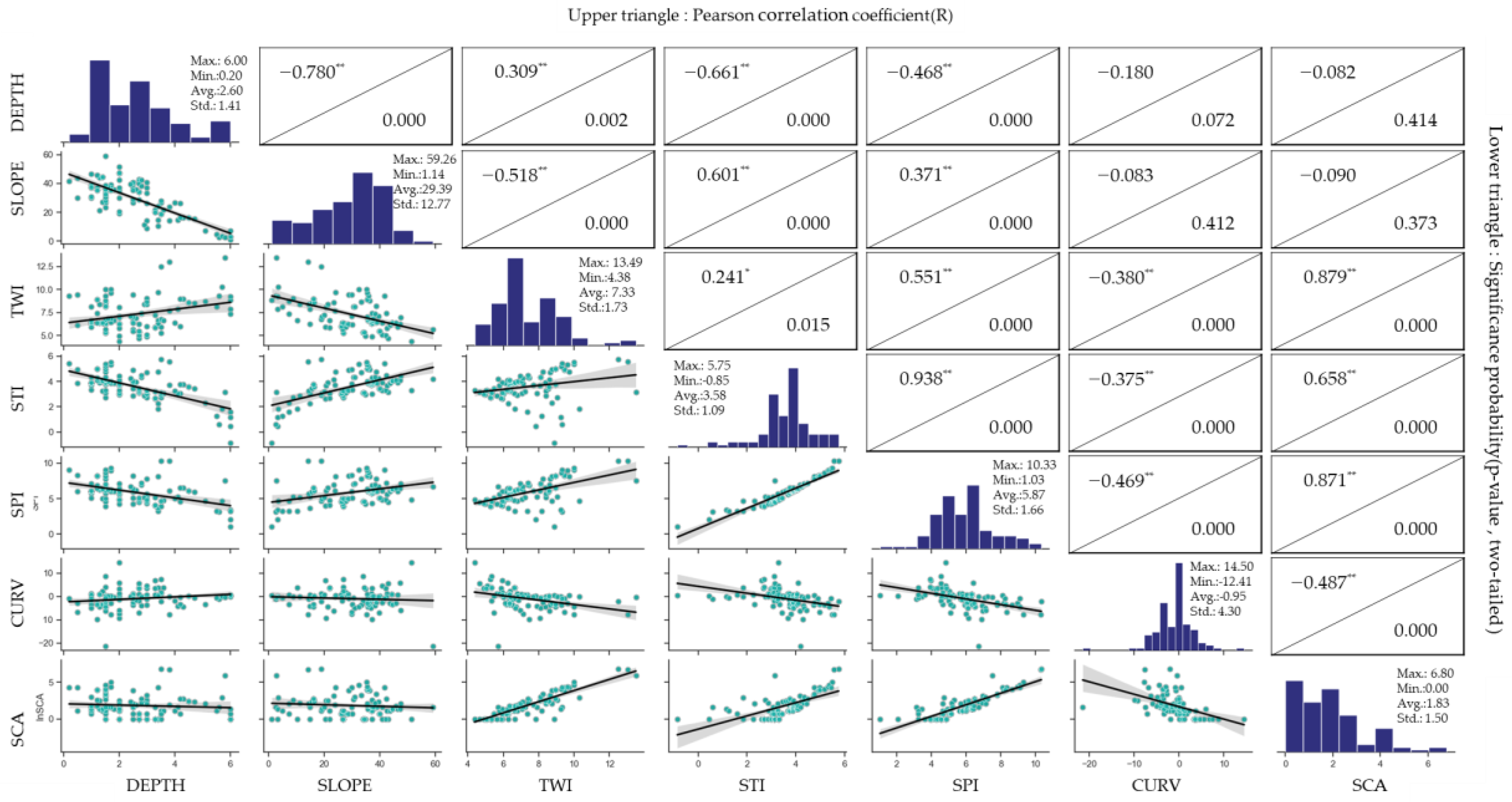
2.2.1. Correlation Analysis

Public drilling data from the Geotechnical Information DB System is used to acquire soil depth data of the study area. This database includes drilling information for 332,889 holes in Korea [51]. In order to secure the reliability of variables which are overly sensitive to the streamline among TAs, data near the streamline were excluded. In addition, too old data (produced before 2000) or data, in which location information of digital maps and boring test data is inconsistent were excluded, since it can be considered an outlier.
Yoon [41] used the soil depth ratio (SR = soil depth/slope height) derived by the slope height for representative rock types in Korea for a total of 373 slopes. It was evaluated and reported that the average soil depth ratio (SR) was 0.09 for sedimentary rocks, 0.17 for metamorphic rocks, and 0.3 for igneous rocks. As such, the weathering depth will be different depending on the rock types, and the soil depth will also be different for this reason. Therefore, in this study, the Boring Test data in study area was classified into igneous, metamorphic, and sedimentary rocks, which are representative rock types in Korea, and the correlation between soil depth and TAs are analyzed. After the excluding outliners, a total of 297 sites were obtained. They were classified into 101 sites for igneous rock, 101sites for metamorphic rock, and 95 sites for sedimentary rock. Descriptive statistics for soil depth by representative rock types are shown in Figure 2. The used soil depth data range from 0.2 to 0.68 m, and the average depth ranges from 2.63 to 3.03 m. In particular, the sedimentary rock data is distributed relatively wide compared to the data for the other two types of rock.
Correlation analysis is performed between the soil depth of the study area and the calculated TAs. The correlation analysis results for each of the representative rock types are shown in Figure 3, Figure 4 and Figure 5 in the form of a correlation matrix. It shows the histograms of each parameter along the central diagonal, the scatter diagram for each pair of parameters in the lower triangle, and each Pearson correlation coefficient and significance level (p-value) is shown in the upper triangle. The results of the correlation analysis indicate that the correlation between soil depth and SLOPE is the highest in all three rock types, and the correlation between Curvature and SCA (Specific catchment area) is relatively low.

2.2.2. Multi-Collinearity Analysis

When there is a high correlation between the independent variables in the multi-regression calculation, the problems of multi-collinearity may occur, which may decrease reliability of the regression coefficient estimates. Multi-collinearity can be evaluated through a variance inflation factor (VIF) such as that given in Equation (1).
Tolerance = 1 R 2 ,   VIF = Tolerance 1
The larger the VIF, the smaller the tolerance, and the more likely it is multicollinear. If the VIF is greater than 5, it is judged that the possibility of multi-collinearity is high. In general, if the VIF is greater than 10, it is determined that multi-collinearity is problematic [52].
Multi-collinearity analysis is performed on six cases consisting of linear regression expressions of six TAs, which are classified into three types of representative rock (Table 2). Table 2 shows the results of the analysis by sequentially removing variables that cause multi-collinearity problems. As a result of the analysis, there is a multi-collinearity problem in Case No. 1 and 2, and Case No. 3–6 have a VIF of 4 or less. Thus, there is no multi-collinearity problem.

2.2.3. Multi-Linear Regression Analysis

Multiple regression analysis is one of the statistical methods used to establish and model the relationship between two or more independent variables for one dependent variable. If the data are linearly related, the multi-linear regression (MLR) of the observation ' y ' for ‘ n ’ independent variables ‘ x ’ is as follows:
y = x _ · β _ + ε = β 0 + β 1 x 1 β n x n + ε  
where β 0 represents the intercept, and β 1 β n represent the regression coefficients. ε is an error that is not explained by the model and is assumed to follow a normal distribution with a mean of zero and a variance of σ 2 . Estimates of regression coefficients can be obtained by β ^ = x _ T x _ 1 x _ T y .
The selection of appropriate independent variables for multi-regression analysis is one of the critical issues. Generally, the methods of selecting independent variables include forward selection, backward elimination, stepwise method, and so on. However, the regression equation does not necessarily include the selected variables. If multi-collinearity exists between the independent variables, another model can be selected without a separate analysis.
Helsel and Hirsch [53] described the existing selection method and its shortcomings. They stated that there are many advantages of choosing a suitable model by evaluating the combination of statistics used in model selection and independent variables used in the model.
In this study, the adjusted coefficient of determination ( R a d j 2 ) and RMSE are used to determine the number of variables to be used in the soil depth prediction model.
The coefficient of determination is a statistic that indicates the model’s suitability for a given dataset. Therefore, the large value of the coefficient of determination means that the proportion of changes that the independent variable can explain is large. However, the coefficient of determination may be increased by some independent variables having high explanatory power, even if some of the independent variables in the model are not very descriptive. There is a correction coefficient as a statistic that complements these shortcomings of the adjusted coefficient of determination ( R a d j 2 ) and is defined as follows:
R a d j 2 = 1 1 R 2 n 1 / n k 1
where n is the number of points in the data sample, k is the number of independent variables included in the regression equation and is the number of variables in the model excluding the constant. These R a d j 2   can be used to compare the suitability of the model [54].
Additionally, it is the most widely used method through RMSE (root mean squared residual) for error analysis of regression models, and the definition is given as Equation (4).
R M S E = i = 1 n Y m i Y p i 2 / n
where Y m is the measurement value, Y p is the predicted value, n is the number of datapoints.
To determine a suitable model, R 2 , R a d j 2 , RMSE for each case are calculated as Table 3, and the results are shown in Figure 6
(1)
As the number of variables used in the model decreases, R a d j 2 decreases: Especially, a large decrease in Cases No. 5 and 6.
(2)
Since Cases No. 1 and 2 have multi-collinearity problems, suitable models are Cases No. 3 and 4.
(3)
Case No. 4, compared to Case No. 3, has a relatively large error.
(4)
Applied Model in this study is Case No. 4, since it uses fewer variables than in Case No. 3.

3. Predicted Soil Depth Model

Previous studies to predict soil depth using TAs have been attempted continuously, and as a result, statistical models for soil depth prediction have been proposed. Representative statistical models for soil depth prediction are summarized in Table 4.
The soil depth prediction model derived in this study is shown in Table 5, and the soil depth prediction model results for the study area are shown in Figure 7a. In addition, the scatter plot for each representative rock type is shown in Figure 7b–d. R a d j 2 for representative rock types are 0.698 (Igneous rock), 0.676 (Metamorphic rock), 0.683 (Sedimentary rock), and the RMSE for representative rock types are 0.870 (Igneous rock), 0.876 (Metamorphic rock), and 0.981 (Sedimentary rock).
For the verification of the developed regression equation, the measurement data and regression equation are compared with the data for the three regions not included in the development of the regression model. The soil depth distribution of the target area is prepared (Table 6). The numbers of data in igneous, metamorphic, and sedimentary rock areas for verification are 18, 30, and 29 sites, respectively, and the determinants between regression and instrumentation data are 0.867, 0.801, and 0.814, respectively. Additionally, R a d j 2 for representative rock types are 0.859 (Igneous rock), 0.794 (Metamorphic rock), 0.807 (Sedimentary rock), and RMSE for representative rock types are 0.724 (Igneous rock), 1.104 (Metamorphic rock), 0.288 (Sedimentary rock).
The distribution of soil depth for the entire area to be verified (Figure 8a,c,e) and the model verification results for each rock distribution (Figure 8b,d,f) are shown in the below figures. As a result of the verification, the R a d j 2   is from 0.794 to 0.859, which is judged to be an appropriately predictable model. However, RMSE is relatively large in metamorphic rock regions. It is considered that this is because the soil depth data of the metamorphic rock verification in the target area are too concentrated near the valley, and a significant amount of the data includes values measured inside the valley.

4. Conclusions

This paper proposes a statistical model that can predict soil depth, an essential factor in landslide disasters. Since erosion and weathering characteristics depend on the rock type, a soil depth prediction model for each rock type was developed: igneous rock, metamorphic rock, and sedimentary rock.
-
The regression model uses open data provided by the Geotechnical Information DB System; a total of 297 sites were obtained. They were classified into 101 sites for igneous rock, 101 for metamorphic rock, and 95 for sedimentary rock.
-
As a result of analyzing the correlation between the six TAs obtained from the numerical map and soil depth, the variables with the highest correlation are SLOPE, and curvature and SCA are found to have relatively low correlation. In addition, a model using three variables (SLOPE, STI, TWI) is determined from R a d j 2 , and RMSE values for multi-collinearity analysis and the combination of six cases for variables.
-
For the models of igneous rock, metamorphic rock, and sedimentary rock, the R a d j 2 values are 0.698, 0.676, and 0.683, respectively, and the RMSE values are 0.870, 0.876, and 0.981. Additionally, Verification sites used data from 18 igneous rock sites, 37 metamorphic rock sites and 30 sedimentary rock sites. The R a d j 2 values are 0.859, 0.794, 0.807, and the RMSEs are 0.724, 1.104, 0.288 for igneous, metamorphic, and sedimentary rocks, respectively.
Therefore, it is expected that the three types of soil depth prediction models proposed will have better applicability and utilization for soil in Korea. However, the data used in this paper are open data provided by the Geotechnical Information DB System and are rather less in number to represent the wide study area. In addition, it should be noted that the relationship between TAs and soil depth used for model development was developed, assuming a linear correlation.

Author Contributions

Formal analysis, investigation, validation, writing—original draft preparation, J.K.; Conceptualization, methodology, writing—review and editing, H.S. All authors have read and agreed to the published version of the manuscript.

Funding

This research was funded by Research Fund of University of Ulsan grant number 2020-0619.

Institutional Review Board Statement

Not applicable.

Informed Consent Statement

Not applicable.

Data Availability Statement

Data is contained within the article.

Conflicts of Interest

The authors declare no conflict of interest.

References

  1. Kuriakose, S.L.; Devkota, S.; Rossiter, D.G.; Jetten, V.G. Prediction of soil depth using environmental variables in an anthropogenic landscape, a case study in the Western Ghats of Kerala, India. CATENA 2009, 79, 27–38. [Google Scholar] [CrossRef]
  2. Mehnatkesh, A.; Ayoubi, S.; Jalalian, A.; Sahrawat, K. Relationships between soil depth and terrain attributes in a semi arid hilly region in western Iran. J. Mt. Sci. 2013, 10, 163–172. [Google Scholar] [CrossRef]
  3. Sarkar, S.; Roy, A.; Martha, T. Soil depth estimation through soil landscape modelling using regression kriging in a Himalayan terrain. Int. J. Geogr. Inf. Sci. 2013, 27, 2436–2454. [Google Scholar] [CrossRef]
  4. Qiyong, Y.; Zhang, F.; Jiang, Z.; Li, W.; Zhang, J.; Zeng, F.; Li, H. Relationship between soil depth and terrain attributes in karst region in Southwest China. J. Soils Sediments 2014, 14, 1568–1576. [Google Scholar] [CrossRef]
  5. Dietrich, W.E.; Reiss, R.; Hsu, M.-L.; Montgomery, D.R. A process-based model for colluvial soil depth and shallow landsliding using digital elevation data. Hydrol. Process. 1995, 9, 383–400. [Google Scholar] [CrossRef]
  6. Minasny, B.; McBratney, A.B. A rudimentary mechanistic model for soil production and landscape development. Geoderma 1999, 90, 3–21. [Google Scholar] [CrossRef]
  7. Yoon, W.S.; Jeong, U.J.; Choi, J.W.; Kim, J.H.; Kim, W.Y.; Kim, C.S. Slope failure index system based on the behavior characteristics: SFi-system. J. Korean Geotech. Soc. 2002, 18, 23–37. [Google Scholar]
  8. Montgomery, D.R.; Dietrich, W.E. A physically based model for the topographic control on shallow landsliding. Water Resour. Res. 1994, 30, 1153–1171. [Google Scholar] [CrossRef]
  9. Ewen, J.; Parkin, G.; O’Connell, P.E. SHETRAN: Distributed River Basin Flow and Transport Modeling System. J. Hydrol. Eng. 2000, 5, 250–258. [Google Scholar] [CrossRef] [Green Version]
  10. Simoni, S.; Zanotti, F.; Bertoldi, G.; Rigon, R. Modelling the probability of occurrence of shallow landslides and channelized debris flows using GEOtop-FS. Hydrol. Process. 2008, 22, 532–545. [Google Scholar] [CrossRef]
  11. Baum, R.L.; Godt, J.W. Early warning of rainfall-induced shallow landslides and debris flows in the USA. Landslides 2010, 7, 259–272. [Google Scholar] [CrossRef]
  12. Uchida, T.; Tamur, K.; Akiyama, K. The role of grid cell size, flow routing algolithm and spatial variability of soil depth on shallow landslide prediction. Ital. J. Eng. Geol. Environ. 2011, 11, 149–157. [Google Scholar] [CrossRef]
  13. Wu, W.; Sidle, R.C. A Distributed Slope Stability Model for Steep Forested Basins. Water Resour. Res. 1995, 31, 2097–2110. [Google Scholar] [CrossRef]
  14. Rosso, R.; Rulli, M.C.; Vannucchi, G. A physically based model for the hydrologic control on shallow landsliding. Water Resour. Res. 2006, 42, 1–16. [Google Scholar] [CrossRef]
  15. Talebi, A.; Uijlenhoet, R.; Troch, P. A low-dimensional physically based model of hydrologic control of shallow landsliding on complex hillslopes. Earth Surf. Process. Landf. 2008, 33, 1964–1976. [Google Scholar] [CrossRef]
  16. Pack, R.; Tarboton, D.; Goodwin, C. The SINMAP approach to terrain stability mapping. In Procedeengs of the 8th Congress of the International Association of Engineering Geology, Vancouver, BC, Canada, 21–25 September 1998. [Google Scholar]
  17. Borga, M.; Dalla Fontana, G.; Cazorzi, F. Analysis of topographic and climatic control on rainfall-triggered shallow landsliding using a quasi-dynamic wetness index. J. Hydrol. 2002, 268, 56–71. [Google Scholar] [CrossRef]
  18. Casadei, M.; Dietrich, W.; Miller, N. Testing a model for predicting the timing and location of shallow landslide in soil-mantled landscapes. Earth Surf. Process. Landf. 2003, 28, 925–950. [Google Scholar] [CrossRef]
  19. Freer, J.; McDonnell, J.J.; Beven, K.J.; Peters, N.E.; Burns, D.A.; Hooper, R.P.; Aulenbach, B.; Kendall, C. The role of bedrock topography on subsurface storm flow. Water Resour. Res. 2002, 38, 5-1–5-16. [Google Scholar] [CrossRef] [Green Version]
  20. Stieglitz, M.; Shaman, J.; McNamara, J.; Engel, V.; Shanley, J.; Kling, G.W. An approach to understanding hydrologic connectivity on the hillslope and the implications for nutrient transport. Glob. Biogeochem. Cycles 2003, 17. [Google Scholar] [CrossRef]
  21. The Role of the Equilibrium Concept in the Interpretation of Landforms of Fluvial Erosion and Deposition; Ahnert, F. (Ed.) University of Liege: Liege, France, 1967. [Google Scholar]
  22. Kooi, H.; Beaumont, C. Escarpment evolution on high-elevation rifted margins: Insights derived from a surface processes model that combines diffusion, advection, and reaction. J. Geophys. Res. 1994, 99, 12191–12209. [Google Scholar] [CrossRef]
  23. Howard, A.D. Badland Morphology and Evolution: Interpretation Using a Simulation Model. Earth Surf. Process. Landf. 1997, 22, 211–227. [Google Scholar] [CrossRef]
  24. Braun, J.; Sambridge, M. Modelling landscape evolution on geological time scales: A new method based on irregular spatial discretization. Basin Res. 1997, 9, 27–52. [Google Scholar] [CrossRef] [Green Version]
  25. Anderson, R.S. Evolution of the Santa Cruz Mountains, California, through tectonic growth and geomorphic decay. J. Geophys. Res. Solid Earth 1994, 99, 20161–20179. [Google Scholar] [CrossRef]
  26. Howard, A.D. A detachment-limited model of drainage basin evolution. Water Resour. Res. 1994, 30, 2261–2285. [Google Scholar] [CrossRef] [Green Version]
  27. Roering, J.; Kirchner, J.; Dietrich, W. Evidence for nonlinear, diffusive sediment transport on hillslopes and implications for landscape morphology. Water Resour. Res. 1999, 35, 853–870. [Google Scholar] [CrossRef] [Green Version]
  28. Gia Pham, T.; Kappas, M.; Van Huynh, C.; Hoang Khanh Nguyen, L. Application of Ordinary Kriging and Regression Kriging Method for Soil Properties Mapping in Hilly Region of Central Vietnam. ISPRS Int. J. Geo-Inf. 2019, 8, 147. [Google Scholar] [CrossRef] [Green Version]
  29. Sitharam, T.G.; Samui, P.; Anbazhagan, P. Spatial Variability of Rock Depth in Bangalore Using Geostatistical, Neural Network and Support Vector Machine Models. Geotech. Geol. Eng. 2008, 26, 503–517. [Google Scholar] [CrossRef]
  30. Tye, A.M.; Lawley, R.L.; Ellis, M.A.; Rawlins, B.G. The spatial variation of weathering and soil depth across a Triassic sandstone outcrop. Earth Surf. Process. Landf. 2011, 36, 569–581. [Google Scholar] [CrossRef] [Green Version]
  31. Chung, J.-w.; Rogers, J.D. Estimating the position and variability of buried bedrock surfaces in the St. Louis metro area. Eng. Geol. 2012, 126, 37–45. [Google Scholar] [CrossRef]
  32. Odeh, I.O.A.; McBratney, A.B.; Chittleborough, D.J. Further results on prediction of soil properties from terrain attributes: Heterotopic cokriging and regression-kriging. Geoderma 1995, 67, 215–226. [Google Scholar] [CrossRef]
  33. Penizek, V.; Boruvka, L. Soil depth prediction supported by primary terrain attributes: A comparison of methods. Plant Soil Environ. 2006, 52, 424–430. [Google Scholar] [CrossRef]
  34. Catani, F.; Segoni, S.; Falorni, G. An empirical geomorphology-based approach to the spatial prediction of soil thickness at catchment scale. Water Resour. Res. 2010, 46. [Google Scholar] [CrossRef] [Green Version]
  35. Liu, J.; Chen, X.; Lin, H.; Liu, H.; Song, H. A simple geomorphic-based analytical model for predicting the spatial distribution of soil thickness in headwater hillslopes and catchments. Water Resour. Res. 2013, 49, 7733–7746. [Google Scholar] [CrossRef]
  36. Sun, W.; Minasny, B.; McBratney, A. Analysis and prediction of soil properties using local regression-kriging. Geoderma 2012, 171–172, 16–23. [Google Scholar] [CrossRef]
  37. Kalivas, D.; Triantakonstantis, D.P.; Kollias, V.J. Spatial prediction of two soil properties using topographic information. Glob. Nest Int. J. 2002, 4, 41–49. [Google Scholar]
  38. McBratney, A.B.; Mendonça Santos, M.L.; Minasny, B. On digital soil mapping. Geoderma 2003, 117, 3–52. [Google Scholar] [CrossRef]
  39. Mueller, T.; Pierce, F. Soil Carbon Maps: Enhancing Spatial Estimates with Simple Terrain Attributes at Multiple Scales. Soil Sci. Soc. Am. J. SSSAJ 2003, 67, 258–267. [Google Scholar] [CrossRef]
  40. Goodman, A. Trend Surface Analysis in the Comparison of Spatial Distributions of Hillslope Parameters; Deakin University: Geelong, VIC, Australia, 1999. [Google Scholar]
  41. Gessler, P.E.; Moore, I.D.; McKenzie, N.J.; Ryan, P.J. Soil-landscape modelling and spatial prediction of soil attributes. Int. J. Geogr. Inf. Syst. 1995, 9, 421–432. [Google Scholar] [CrossRef]
  42. Statistics-Korea. Population Projections for Provinces (2017~2047). Available online: http://kostat.go.kr/portal/eng/pressReleases/8/8/index.board?bmode=read&aSeq=377503&pageNo=&rowNum=10&amSeq=&sTarget=&sTxt= (accessed on 15 August 2022).
  43. National Geographic Information Institute. Available online: https://www.ngii.go.kr/ (accessed on 25 May 2022).
  44. Shary, P.A. Land surface in gravity points classification by a complete system of curvatures. Math. Geol. 1995, 27, 373–390. [Google Scholar] [CrossRef]
  45. Moore, I.D.; Grayson, R.B.; Ladson, A.R. Digital terrain modelling: A review of hydrological, geomorphological, and biological applications. Hydrol. Process. 1991, 5, 3–30. [Google Scholar] [CrossRef]
  46. Florinsky, I.V. An illustrated introduction to general geomorphometry. Prog. Phys. Geogr. Earth Environ. 2017, 41, 723–752. [Google Scholar] [CrossRef]
  47. Beven, K.J.; Kirkby, M.J. A physically based, variable contributing area model of basin hydrology / Un modèle à base physique de zone d’appel variable de l’hydrologie du bassin versant. Hydrol. Sci. Bull. 1979, 24, 43–69. [Google Scholar] [CrossRef]
  48. Moore, I.D.; Burch, G.J. Physical Basis of the Length-slope Factor in the Universal Soil Loss Equation. Soil Sci. Soc. Am. J. 1986, 50, 1294–1298. [Google Scholar] [CrossRef]
  49. Stocking, M.A. Relief Analysis and Soil Erosion in Rhodesia Using Multivariate Techniques. Z. Für Geomorphol. 1972, 16, 432–443. [Google Scholar]
  50. Gallant, J.C.; Hutchinson, M.F. A differential equation for specific catchment area. Water Resour. Res. 2011, 47, W05535. [Google Scholar] [CrossRef] [Green Version]
  51. Geotechnical Information DB System. Available online: https://www.geoinfo.or.kr/ (accessed on 16 August 2020).
  52. Dormann, C.F.; Elith, J.; Bacher, S.; Buchmann, C.; Carl, G.; Carré, G.; Marquéz, J.R.G.; Gruber, B.; Lafourcade, B.; Leitão, P.J.; et al. Collinearity: A review of methods to deal with it and a simulation study evaluating their performance. Ecography 2013, 36, 27–46. [Google Scholar] [CrossRef]
  53. Helsel, D.R.; Hirsch, R.M. Statistical Methods in Water Resources; 04-A3; Elsevier: Reston, VA, USA, 2002; pp. 295–318. [Google Scholar]
  54. Shieh, G. Improved Shrinkage Estimation of Squared Multiple Correlation Coefficient and Squared Cross-Validity Coefficient. Organ. Res. Methods 2007, 11, 387–407. [Google Scholar] [CrossRef]
  55. Han, X.; Liu, J.; Mitra, S.; Li, X.; Srivastava, P.; Guzman, S.M.; Chen, X. Selection of optimal scales for soil depth prediction on headwater hillslopes: A modeling approach. CATENA 2018, 163, 257–275. [Google Scholar] [CrossRef]
Figure 1. Location of study area and distribution of soil depth sampling sites.
Applsci 13 01453 g001
Figure 2. Descriptive statistics on three representative rock types sampled in the study area (Gangwon region).
Applsci 13 01453 g002
Figure 3. Correlation matrix for igneous rock (* Significant at the 0.05 probability level. ** Significant at the 0.01 probability level).
Applsci 13 01453 g003
Figure 4. Correlation matrix for metamorphic rock (*: Significant at the 0.05 probability level. **: Significant at the 0.01 probability level).
Applsci 13 01453 g004
Figure 5. Correlation coefficient for Sedimentary rock (*: Significant at the 0.05 probability level. **: Significant at the 0.01 probability level).
Applsci 13 01453 g005
Figure 6. Comparison results of six regression models for selecting suitable models.
Applsci 13 01453 g006
Figure 7. The proposed statistical prediction models result in the study area, (a) The soil depth map, Scatterplots showing the relationship between predicted and measured soil depth for (b) Igneous rock ( R 2 = 0.702), (c) Metamorphic rock ( R 2 = 0.686), (d) Sedimentary rock ( R 2 = 0.693).
Applsci 13 01453 g007
Figure 8. The proposed statistical prediction models result in the verification sites, The soil depth map for (a) Igneous rock, (c) Metamorphic rock (e) Sedimentary rock, and Scatterplots showing the relationship between predicted and measured soil depth for (b) Igneous rock ( R 2   = 0.867), (d) Metamorphic rock ( R 2 = 0.801), (f) Sedimentary rock ( R 2 = 0.814).
Applsci 13 01453 g008
Table 1. Definition of Terrain Attributes in the study area and its derived results.
Terrain AttributesDefine
Applsci 13 01453 i001The SLOPE is defined as the angle between the tangent to the terrain surface and the horizontal plane and is a variable that determines the flow velocity by gravity [44].
β = arctan p 2 + q 2   where   p = z x ,   q = z y
Applsci 13 01453 i002Topographic Wetness Index (TWI) is an index of the water content in the ground, and it can determine the spatial pattern of water flow [45,46]. TWI was developed by Beven and Kirkby [47] in TOPMODEL and is defined as a function of the upstream contributing area per unit area orthogonal to the slope and the flow direction.
ln α tan β
Where α is the slope area of the unit grid length, β is the slope at a point on the surface.
Applsci 13 01453 i003Sediment Transport Index (STI) was proposed by Moore and Burch [48], and is an indicator of the erosion and sedimentation process. It is defined by the non-linear equation of the specific catchment area and slope.
L S = A S 22.13 0.6 sin β 0.0896 1.3
where A S is a specific catchment area, β is the slope at a point on the surface.
Applsci 13 01453 i004Stream Power Index (SPI) is an index indicating the erosion risk of potential flows on a terrain surface. When the catchment area and slope increase, the SPI also increases as the flow velocity due to gravity increases [45,46] The SPI is defined by the following equation.
S P I = ln A s × tan β
Applsci 13 01453 i005Curvature has an important effect on landslides and is classified into three types: convex, plane, and concave. In general, it is considered to have a negative effect on the landslide due to ponding caused by more extreme rainfall penetration in the case of the concave curvature relative to that of the Convex [49].
Applsci 13 01453 i006Specific catchment area (SCA) is defined as the value obtained by dividing the upslope area by the contour width and is a value commonly used in hydrology to analyze the flow of water on the slope [50].
A s = lim w 0 A w
Table 2. The result of multi-collinearity analysis.
Case No.ParameterIgneous RockMetamorphic RockSedimentary Rock
ToleranceVIFToleranceVIFToleranceVIF
1SLOPE0.01282.0700.01096.0590.2703.706
TWI0.002591.4250.002523.3600.02146.671
STI *0.0011166.3740.0011089.2550.02737.516
SPI0.0011836.4030.0002307.4410.06116.270
CURV0.7311.3680.7001.4290.9371.068
SCA **0.01566.5950.01376.4710.03230.870
2SLOPE0.1218.2870.1427.0480.2703.699
TWI0.01663.4260.01856.2470.02737.110
STI *0.06216.0750.06814.7080.05518.134
CURV0.7381.3550.7401.3520.9411.063
SCA **0.01566.0080.01472.5810.03230.814
3SLOPE0.1417.0750.1675.9750.2713.695
TWI0.2663.7630.2304.3510.5381.859
STI *0.2394.1810.2214.5160.3842.604
CURV0.7791.2840.7491.3350.9611.040
4SLOPE0.1417.0740.1725.8090.2723.678
TWI0.2823.5450.2543.9390.5451.833
STI *0.2444.1070.2214.5150.3892.573
5SLOPE0.5771.7330.6391.5660.5561.798
TWI0.5771.7330.6391.5660.5561.798
6SLOPE1.0001.0001.0001.0001.0001.000
* ln(STI), ** ln(SCA).
Table 3. The results of the multi-collinearity analysis.
Case No.Igneous RockMetamorphic RockSedimentary Rock
R 2 R a d j 2 RMSE R 2 R a d j 2 RMSE R 2 R a d j 2 RMSE
10.7070.6880.8630.6970.6770.7730.8560.8460.672
20.7040.6890.8660.6910.6740.7810.6980.6810.973
30.7040.6910.8680.6900.6780.7810.6950.6820.977
40.7020.6930.8700.6860.6760.8760.6930.6830.981
50.6650.6580.9220.6660.6590.8640.6210.6131.09
60.6070.6030.9990.6090.6050.8780.6040.6001.114
Case 1: SLOPE, TWI, STI*, SPI, CURV, SCA**, Case 2: SLOPE, TWI, STI*, CURV, SCA**, Case 3: SLOPE, TWI, STI*, CURV, Case 4: SLOPE, TWI, STI*, Case 5: SLOPE, TWI, Case 6: SLOPE.
Table 4. Previously proposed statistical soil depth prediction models.
ProposerModelRange of Soil Thicknesses (cm)Number of
Datapoints
Penizek [33] 88.8 + 1.020 AS + 0.057 AL 2.491 S 40–160553
Gessler [41] 57.95 + 12.83 CV PL + 21.46 TWI 0–20030
Qiyong [4] 97.883 1.457 S + 2.688 TWI 0.073 AL 3.1–198.4137
Han [55] 17.918 TWI + 0.550 (Cell size = 10m)30–15079
Mehnatkesh [2] 122.13 0.11 S + 0.012 TWI + 0.012 CA 0.23 STI 30–150100
AS: Aspect, AL: Altitude, S: Slope,   CV PL : Plane Curvature.
Table 5. The result of soil depth prediction models in this study.
Rock TypeModelp-ValueNumber of Data
Igneous 0.626 0.536 STI + 0.509 TWI 0.021 SLOPE <0.001101
Metamorphic 4.442 0.702 STI + 0.228 TWI 0.034 SLOPE <0.001101
Sedimentary 4.289 0.667 STI + 0.242 TWI 0.041 SLOPE <0.00195
Table 6. Results of soil depth prediction models at the verification site.
Rock TypeR R 2 R a d j 2 RMSEp-ValueNumber of Datapoints
Igneous0.9310.8670.8590.724<0.00118
Metamorphic0.8950.8010.7941.104<0.00130
Sedimentary0.9020.8140.8070.288<0.00129
Disclaimer/Publisher’s Note: The statements, opinions and data contained in all publications are solely those of the individual author(s) and contributor(s) and not of MDPI and/or the editor(s). MDPI and/or the editor(s) disclaim responsibility for any injury to people or property resulting from any ideas, methods, instructions or products referred to in the content.

