Article

The Experiments and Stability Analysis of Hypersonic Boundary Layer Transition on a Flat Plate

1
Department of Mechanics, School of Mechanical Engineering, Tianjin University, Tianjin 300072, China
2
China Academy of Launch Vehicle Technology, Beijing 100076, China
3
College of Aerospace Engineering, Nanjing University of Aeronautics and Astronautics, Nanjing 210016, China
4
Key Laboratory of Unsteady Aerodynamics and Flow Control, Ministry of Industry and Information Technology, Nanjing University of Aeronautics and Astronautics, Nanjing 210016, China
*
Author to whom correspondence should be addressed.
Appl. Sci. 2023, 13(24), 13302; https://doi.org/10.3390/app132413302
Submission received: 6 November 2023 / Revised: 9 December 2023 / Accepted: 14 December 2023 / Published: 16 December 2023
(This article belongs to the Topic Fluid Mechanics)

Abstract

:
Experimental and linear stability theory (LST) investigation of boundary layer transition on a flat plate was conducted with a flow of Mach number 5. The temperature distributions and second-mode disturbances on the flat plate surface at different unit Reynolds number (Reunit) values were captured by infrared thermography and PCB technology, respectively, which revealed the transition location of the flat-plate boundary layer. The PCB sensors successfully captured the second-mode disturbances within the boundary layer initially at a frequency of about 100 kHz, with a gradually expanding frequency range as the distance travelled downstream increased. The evolution characteristics of the second-mode instabilities were also investigated by LST and obtained for the second mode, ranging from 100 to 250 kHz. The amplitude amplification factor (N-factor) of the second-mode instabilities was calculated by the eN method. The N-factor of the transition location in the wind tunnel experiment predicted by LST is about 0.98 and 1.25 for Reunit = 6.38 × 10⁶ and 8.20 × 10⁶, respectively.

1. Introduction

The flow regime within the boundary layer, whether laminar or turbulent, significantly influences surface friction and heat exchange. The friction and heat flux of the turbulent boundary layer are approximately 3~5 times higher than those observed in the laminar boundary layer [1]. Accurate and efficient prediction of boundary layer transition is crucial for enhancing the safety and payload capacity of hypersonic vehicles. Consequently, the precise determination of the transition location in the hypersonic boundary layer is of paramount importance for the meticulous design of the entire aerospace vehicle, especially concerning the thermal protection system (TPS). Nevertheless, due to the inherently highly nonlinear characteristics, the transition of the hypersonic boundary layer remains a formidable challenge in the realm of fluid mechanics [2,3].
In contrast to the incompressible boundary layer, hypersonic boundary layer transition is influenced by two mechanisms: second-mode instability and crossflow instability. Mack [4,5] initially identified the second-mode instability using linear stability analysis to explore the hypersonic flat-plate boundary layer. Subsequent experiments have successfully measured the second mode, and the results align closely with theoretical predictions from linear stability theory (LST) [6,7,8]. Currently, wind tunnel experiments continue to play a crucial role in advancing our understanding of hypersonic boundary layer transition. Zhao et al. [9] studied the influence of different total temperatures on the basic flow and transition position of the boundary layer under the same Mach number and unit Reynolds number freestream conditions and pointed out the significance of ensuring consistent total temperature of the inflow in wind tunnel experiments. With the advancement of measurement technology, some instantaneous measurement methods that have high spatial and temporal resolution, such as PCB [10,11] and ALTP [12], are used for identifying the disturbance modal in the boundary layer. Infrared thermography appears to be a potential tool for investigating boundary layer transitions. Borg et al. [13] employed IR technology to study the boundary layer transition of HIFiRE-5b at a freestream Mach number 6. The findings suggest that IR can clearly depict high- and low-temperature streaks in the streamwise direction on the model surface and capture the transition process. In addition to surface disturbance measurements, some flow visualization techniques are used to capture the process of boundary layer transition, too. Yao et al. [14] used infrared thermography and wall pressure tests to obtain the turning position and the development and interaction law of unstable modes of a flat delta wing in a hypersonic wind tunnel. Xu et al. [15] successfully captured the process of the second-mode wave growth and breaking into turbulence in the boundary layer of a conical surface using NPLS technology and found that a single forward-facing step (FFS) could suppress the second-mode wave and delay the cone’s hypersonic boundary layer transition at AOA 0. Zhu et al. [16] used the Rayleigh scattering technique to successfully capture second modes of rope waves in the boundary layer of a flared cone and found that the amplitude of the second mode decays before transition to turbulence. Liu et al. [17] used infrared thermography to study the effect of different roughness elements on the transition of a flat plate at Mach number 6, with a special study of the roughness element wake vortex structure. In addition to wind tunnel experiments, due to the development of computer computing power, many researchers have begun to use direct numerical simulation (DNS) to study the sensitivity of the hypersonic boundary layer of the flat plate and the propagation of disturbance [18,19].
Various theoretical analysis techniques, including linear stability theory (LST) and parabolized stability equations (PSE), have been employed for the investigation and prediction of hypersonic boundary layer transition. Saric [20] conducted a comprehensive examination of hypersonic boundary layer transition prediction, emphasizing the potential applicability of the eN method for predicting two-dimensional hypersonic transition locations in his work [21]. Additionally, Chen et al. [22] explored boundary layer transition on a cone and plate at Mach number 3.5 using the eN method. Their results indicate that when N = 10, the theoretical results are in excellent agreement with the transition data obtained by the experiments. Juliano et al. [23] investigated the influence of the noise environment on Hifire-5 elliptic cone transition in the wind tunnel and found that N = 3.5 in the case of noise, and N = 8 in the quiet freestream condition. Su et al. [24] improved the eN method while considering the modal transformation; the results show that by neglecting the disturbance decay between the two instability modes, the proposed strategy provides more accurate results than existing strategies. LST method has also been applied to other studies on boundary layer stability. Zhu et al. [25] used wind tunnel experiment and stability analysis to study the nonlinear interaction between high-frequency and low-frequency modes on porous surfaces. It was found that the suppression of near wall disturbances by porous surfaces changed the spatial distribution characteristics of fundamental resonance disturbances, broke the phase-locked relationship, and suppressed the instability of fundamental oblique waves. At the same time, the study also found that porous surfaces greatly suppressed aerodynamic heating and delayed the transition position. Chen et al. [26] developed a linear stability analysis method under thermochemical nonequilibrium conditions, which extends the scope of application of linear stability. In a recent study, Klothakis et al. [27] employed the direct simulation Monte Carlo (DSMC) method to computationally analyze the steady laminar flow over a semi-infinite flat plate. The obtained results demonstrated a favorable agreement with corresponding solutions derived from boundary layer considerations. Following this, the researchers conducted a comparative examination of the linear stability characteristics between the DSMC-generated basic flow and those derived from classical Navier–Stokes-based profiles. The findings revealed a slight increase in stability for flows obtained through the DSMC method when compared to their Navier–Stokes counterparts.
In this study, experimental investigations were conducted to examine hypersonic boundary layer transition on a flat plate, employing infrared (IR) thermography and PCB technology. Additionally, linear stability analysis was employed to calculate the growth rate of the second-mode instability in the boundary layer across various Reynolds numbers. The primary focus of this paper centers on characterizing the transition position observed in the experiments, along with analyzing the growth rate and amplitude of disturbances within the hypersonic boundary layer. Furthermore, the determination of the N-factor at the transition location of the flat plate in the NHW hypersonic wind tunnel was performed using the eN method.

2. Experiment Facility and Model
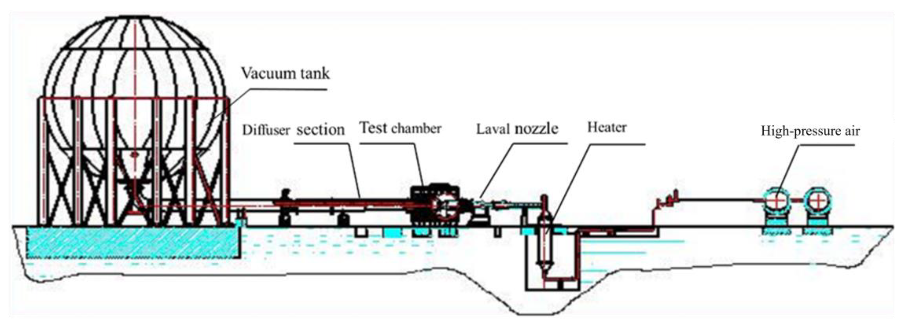
2.1. Wind Tunnel

The experimental investigations were carried out by using the hypersonic wind tunnel (NHW) at Nanjing University of Aeronautics and Astronautics. This wind tunnel operates in a blow-down and vacuum-suction mode, allowing for a variable operating Mach number ranging from 4 to 8 through adjustments to the corresponding Laval nozzle, as shown in Figure 1. The wind tunnel is equipped with five sets of axisymmetric Laval nozzles, each with a 500 mm diameter, enabling the provision of a stable flow field at Mach number 5 for approximately 8 s during experimental procedures. Optical accessibility is facilitated by two optical windows on each side of the plenum chamber, suitable for schlieren imaging. Additionally, a rectangular window situated above the plenum chamber serves as an optical access point for high-speed cameras or infrared cameras.

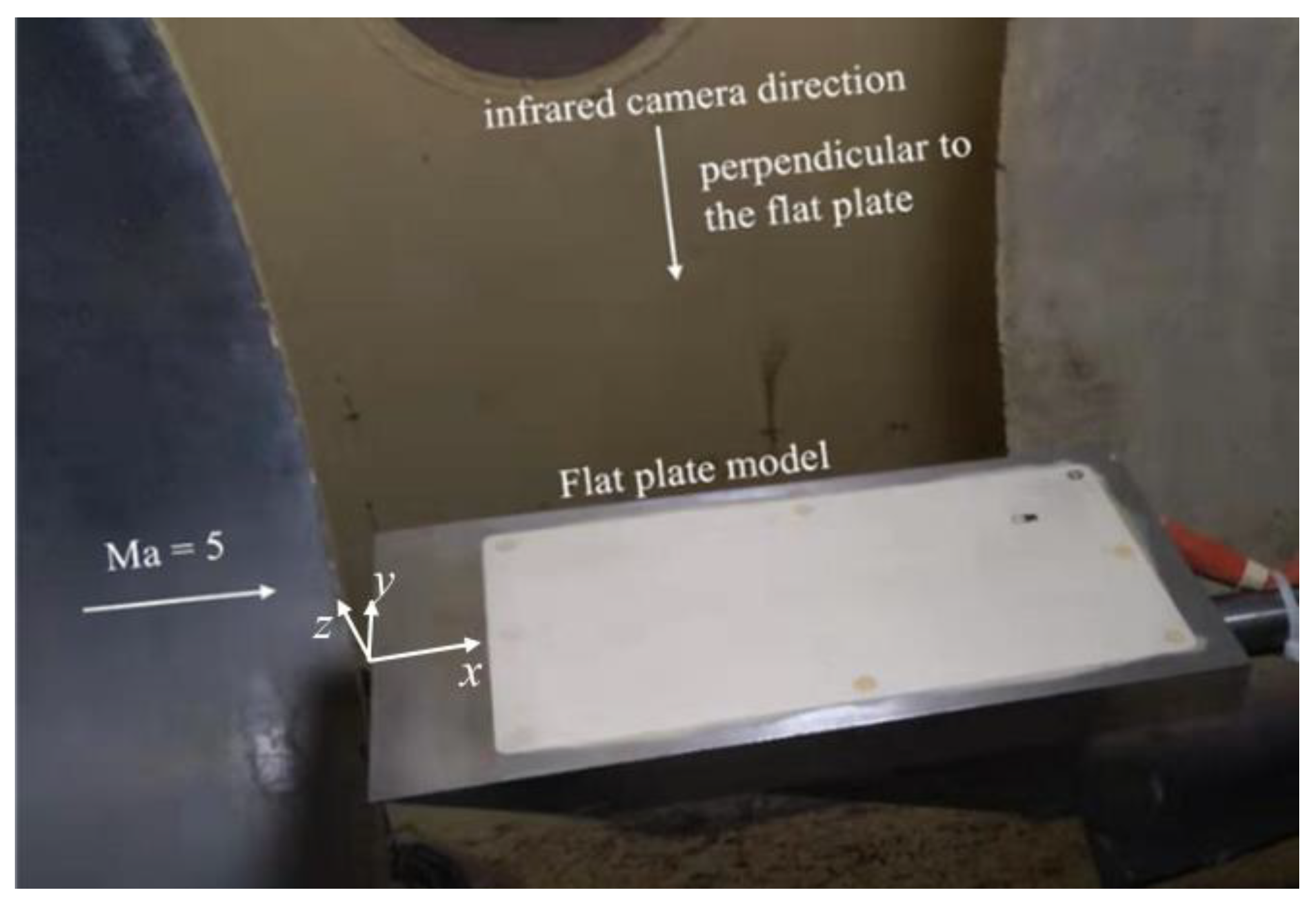
2.2. Experiment Model

Figure 2 displays a photograph of the flat-plate model positioned within the wind tunnel at a zero angle of attack. The primary structure of the model is constructed from stainless steel to guarantee adequate stiffness. Positioned centrally within the model is an embedded polyether ether ketone (PEEK) component. PEEK is a high-temperature-resistant, high-strength resin material with excellent insulation performance. By utilizing the insulation performance of PEEK material, the strength of high-speed airflow and wall friction can be well reflected on the surface temperature of the model, making it convenient for monitoring by infrared thermal imagers. In addition, PEEK also has a high infrared emissivity, making the results monitored by the infrared thermal imager highly accurate, which makes it very suitable for the application of IR thermography. Juliano et al. [23] used infrared thermal imaging technology to study the surface transition phenomenon of the HIFiRE-5 model made of polyether ether ketone (PEEK) material under Ma = 6 conditions. The experimental results showed that the infrared thermal image can clearly display the high- and low-temperature bands flowing towards the model surface and can capture the transition process. The Mach 5 freestream direction is from left to right. The infrared camera (FLIR T630sc, FLIR Systems Inc, American) observes the flat plate from the upper observation hole with a zinc selenide (ZnSe) window. The detailed flow conditions in experiment are shown in Table 1; Ma, P0, T0, and Re/m are the freestream Mach number, freestream stagnation pressure, freestream stagnation temperature, and freestream unit Reynolds number, respectively. The unit Reynolds number is changed by adjusting the total pressure of the freestream flow. Three freestream flow conditions with different Reynolds numbers were set up to study the effect of unit Reynolds number on transition Reynolds number.

2.3. Heat Flux Calculating

In this experiment, the heat flux distribution on the surface of the plate was obtained by solving the one-dimensional inverse heat-transfer equation [28]. The surface temperature of the model was recorded by IR image. A constant initial temperature was assumed through the PEEK. According to the one-dimensional heat conduction equation,
T t = α 2 T y 2
where α is the thermal diffusivity, which is related to the materials. In Equation (1), the time term adopts the first-order forward difference, and the space term adopts the second-order central difference scheme. The finite difference scheme is presented as follows:
T i + 1 , j T i , j t = α ( T i , j 1 2 T i , j + T i , j + 1 ) ( y ) 2
Δy takes the appropriate value to ensure the numerical stability. Utilizing the temperature distribution within the PEEK model, the heat flux for individual pixels at each time step is computed through the application of Fourier’s law, as expressed below [28]:
q = k T y
The dimensionless Stanton number (St) is derived from the surface heat flux by utilizing the freestream parameters.
S t = q ρ U C p ( T 0 T w )
where the subscript ∞ represents the freestream condition. Cp, T0, and Tw represent the constant pressure specific heat, flow total temperature, and wall temperature, respectively.

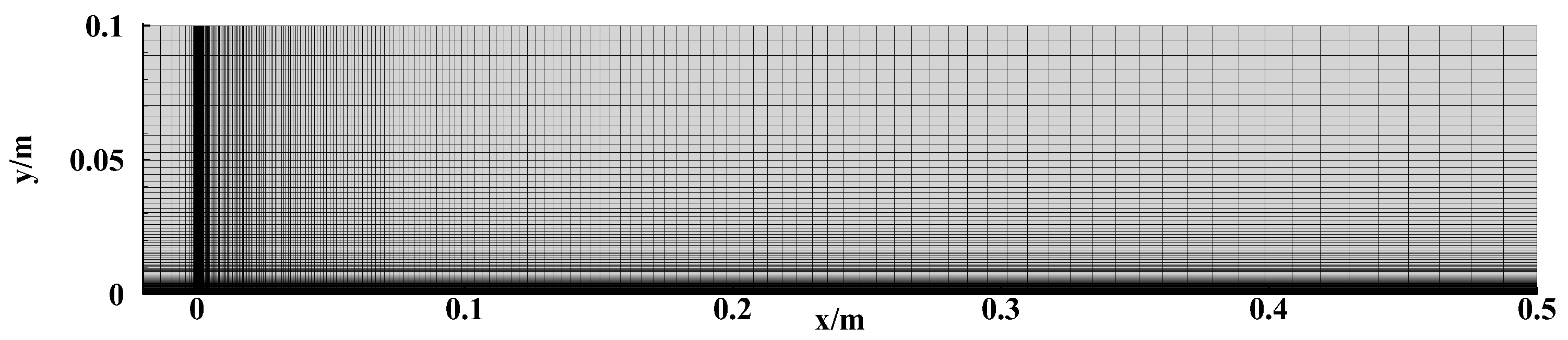
2.4. Numerical Setup

In this investigation, two-dimensional, compressible Navier–Stokes equations are solved utilizing an upwind finite-volume formulation. The transition model employed in all simulations is the k-ω SST model, introduced by Menter [29] to address certain limitations within the realm of two-equation turbulence models. The k-ω SST model integrates the advantages of Wilcox’s k-ω model [30] for capturing turbulent flow near the wall and the characteristics of the k-ε model in regions far from the wall. This integration is achieved through a coupling function, ensuring the conservation of compressible equations for turbulent kinetic energy and specific dissipation rate, respectively.
( ρ k ) t + ( ρ u j k ) x j = τ i j u j x j β k ω + x j [ ρ ( ν + σ k ν T ) k x j ]
and
( ρ ω ) t + ( ρ u j ω ) t = γ ν T τ i j u j x j β ω 2 + x j [ ρ ( ν + σ ω ν T ) ω x j ] + 2 ( 1 F 1 ) ρ σ ω 2 ω k x j ω x j
where β, β*, γ, σk, and σw2 are closure constant coefficients.
The model is completed by the kinematic viscosity limitation of the following form:
ν T = k max ( ω , Ω F 2 a 1 )
where Ω is the vorticity magnitude, a constant coefficient, and a function with asymptotic behavior. Boundary conditions on a smooth wall are as follows:
k ω = 0 , ω w = 10 6 ν β 1 y 2
with β 1 being a constant coefficient.
The numerical calculation model conditions are the same as the experimental conditions, with a length of 0.5 m and a height of 0.1 m. First, we calculate the number of grids to 200 × 150; the height of the first layer of grid on the wall is 1 × 10⁻⁵ m, satisfying y+ less than 1. The schematic diagram of the grid is shown in Figure 3. The incoming flow boundary condition is the pressure far field, the outlet is the pressure outlet boundary condition, and the upper and front areas of the plate are set with symmetric boundary conditions.

2.5. Linear Stability Theory

Linear stability theory (LST) is established under the assumption of small perturbations [4], and under this assumption, the perturbation can be written in the form of the sum of the basic flow and the perturbation quantity:
p ( x , y , z , t ) = p ¯ ( x , y ) + p ( x , y , z , t )
In hypersonic boundary layer, p (x, y, z, t) represents u, v, w, ρ, and T. The basic flow field is obtained by solving the Blasius equation. It is assumed that the flow in the boundary layer is a parallel flow, and the small perturbation p′ can be written in the form of the traveling wave as follows:
p ( x , y , z , t ) = p ( y ) e i ( α x + β z ω t ) + c . c .
where α, β, and ω are the streamwise wave number, the spanwise wave number, and the frequency, respectively. In addition, c.c. represents the conjugate complex number. The generalized eigenvalue problem can be obtained by putting Equation (2) into the wave equation and ignoring the second-order small quantities. The eigenvalue is the streamwise growth rate, and the eigenvector represents the disturbance shape along the wall normal. In spatial mode, β and ω are real numbers, and α is an imaginary number:
α = α r + i α i
The real part represents the wave number of the disturbance, and the imaginary part represents the disturbance growth rate. When αi < 0, the disturbance is unstable along the flow direction.
In the realm of laminar–turbulent transition (LST) analysis, a widely applied approach involves the computation of the N-factor using a semi-empirical method known as the eN method. The determination of the N- factor is calculated by the following formula [23]:
N = x 0 x α i d x
where x0 represents the flow direction position where the disturbance wave first begins to be unstable, and x0 is different at different frequencies. In general, the NT in a low-speed wind tunnel is generally 6~9, while in a hypersonic wind tunnel, the divergence of NT is quite large. In the case of hypersonic flow, the N- factor as the transition criterion needs to be determined by wind tunnel experiments.

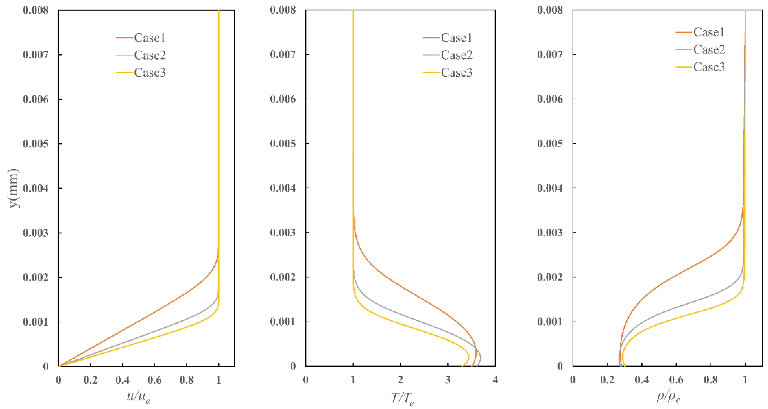
2.6. Steady Base Flow

The calculation of the stability equation requires a high-precision basic flow field. For the flat-plate boundary layer, the basic flow field can be obtained by calculating the compressible boundary layer equation [31]. Wall temperature, Prandtl number, and specific heat ratio are assumed to be constant. The viscosity coefficient adopts the Sutherland viscosity law.
( ρ μ f ) + 1 2 f f = 0 1 2 c p f g + 1 Pr ( κ g ρ ) + ρ μ E c ( f ) 2 = 0 ρ = 1 g
In this paper, the laminar boundary layer flow should be obtained for LST analysis by solving the compressible boundary layer equation. For solving the differentia equations, the physical quantities are nondimensionalized by the free flow parameters and reference length. The dimensionless compressible boundary layer equations are as follows, where Ec, k, and Pr are the Eckert number, thermal conductivity, and Prandtl number, respectively. In this work, we consider the boundary layer of a perfect gas with Prandtl number Pr = 0.71 and specific heat ratio γ = 1.4, and the viscosity law satisfies the Sutherland’s law.
The mean flow variables of the boundary layer at different unit Reynolds numbers are given in Figure 4. As the unit Reynolds number increases, the boundary layer thickness gradually diminishes.

3. Experimental Results and Stability Analyses
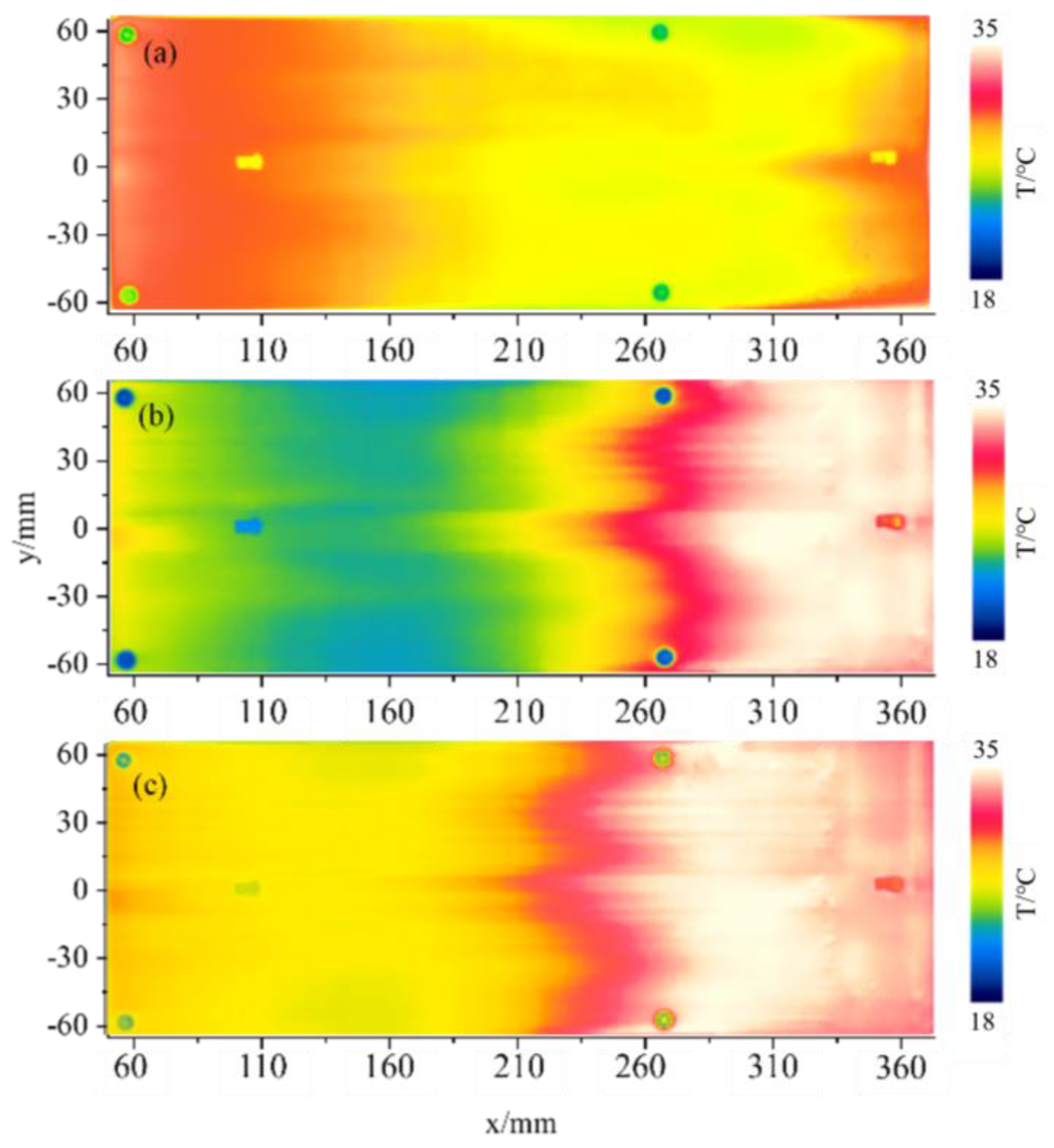
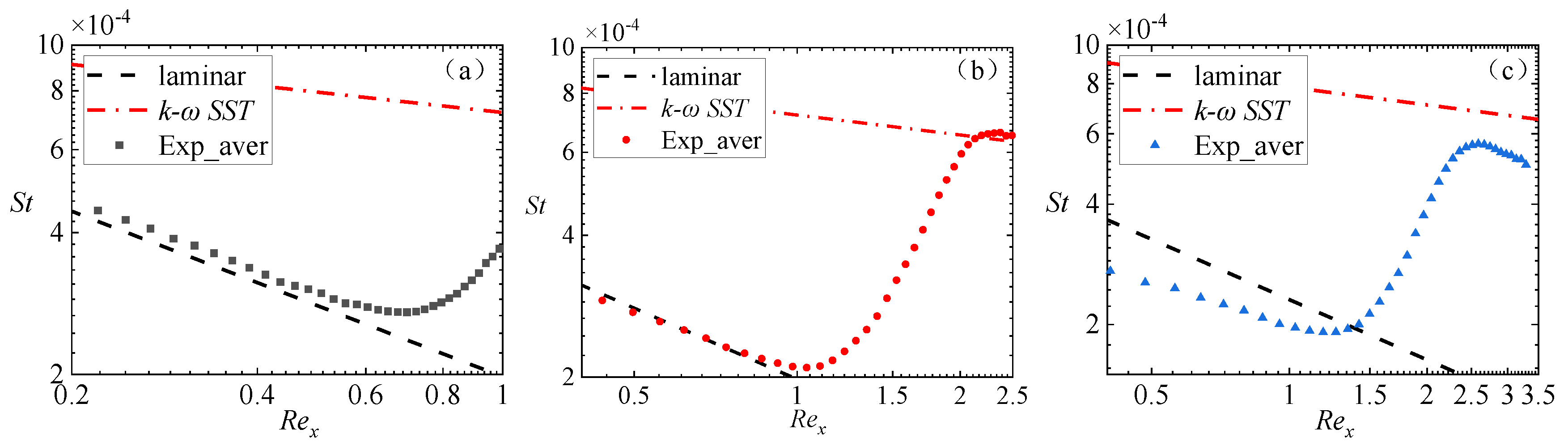
3.1. IR Results

Figure 5 shows the surface temperature distribution of a flat plate under different unit Reynolds numbers. At a lower Reynolds number (Figure 5a), the temperature at the leading edge of the flat plate is the highest and gradually decreases downstream. With the increase in Reynolds number (Figure 5b,c), the plate surface shows a different temperature distribution, and there is an obvious temperature difference along the flow direction. It can be seen from the IR image that the transition region presents an irregular “wavy shape”. Willems et al. [32] also found this “wavy” transition non-uniformity in the study of the boundary layer transition of the flat plate and concluded that it may be caused by the natural incoming flow and the disturbance non-uniformity of the forefront of the flat plate.
The mean Stanton number distributions calculated from IR images are shown in Figure 6. The black and red dashed lines represent the Stanton numbers for the flat-plate boundary layer in all laminar and turbulent states, respectively. The curve of discrete points in the Figure 6 shows the distribution of mean Stanton numbers along the x-direction calculated from the wind tunnel experiments, where the surface of a flat plate develops from laminar flow through turning to turbulence. In the transition region, the Stanton number increases rapidly and reaches the value for turbulent flow. In the case of a lower unit Reynolds number (Figure 6a), limited by the length of the plate, the IR images only capture the beginning of the BL transition. With the increase in the unit Reynolds number, the transition position moves upstream, whereas the transition Reynolds number increases, and the complete laminar transition to turbulent processes can be observed. As a comparison, the results of full laminar flow and full turbulence are also given as a reference. The calculation results of infrared thermal imaging are in good agreement with the calculation results in the laminar flow area, and the change of the flow direction Stanton number is within the range of laminar flow and turbulence.
Figure 7 represents the transition Reynolds number distribution at different spanwise positions under different unit Reynolds numbers. Moreover, the transition Reynolds number calculated by the compressibility-modified transition model γ-Reθt [33] (shown as CC in the Figure 7) is given. It can be found that for the lower unit Reynolds number (Figure 7a), the transition Reynolds number is also relatively small; with the increase in the unit Reynolds number of the freestream, the transition Reynolds number increases accordingly. In addition, it also shows that the spanwise distribution of transition position on the surface of the flat plate is uneven, and the spanwise distribution of transition Reynolds number increases with the increase in the unit Reynolds number, similarly as in Figure 5. In this paper, the unit Reynolds number has a great influence on the transition Reynolds number, whereas some wind tunnel experiments show the opposite results. A more in-depth investigation is warranted to explore the impact of unit Reynolds number on the transition Reynolds number.

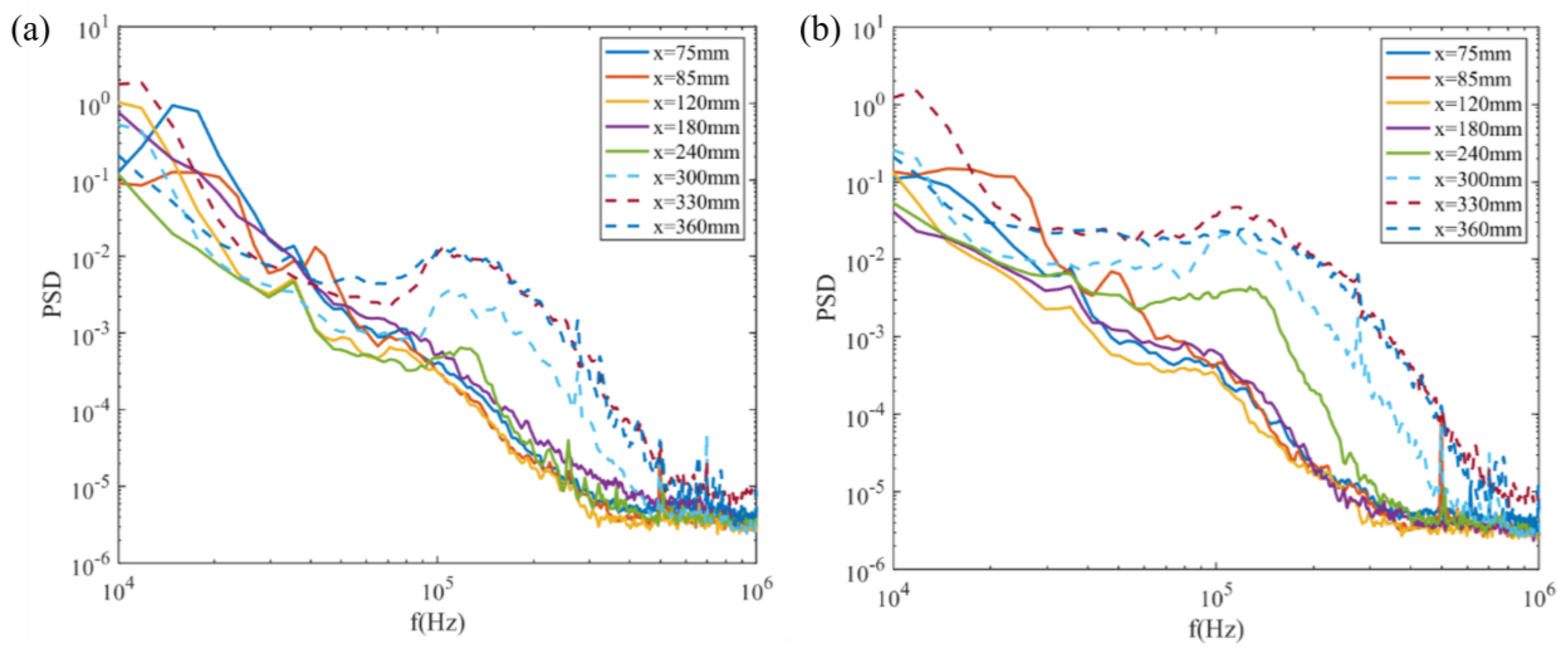
3.2. Instability Characteristics along Streamwise Direction
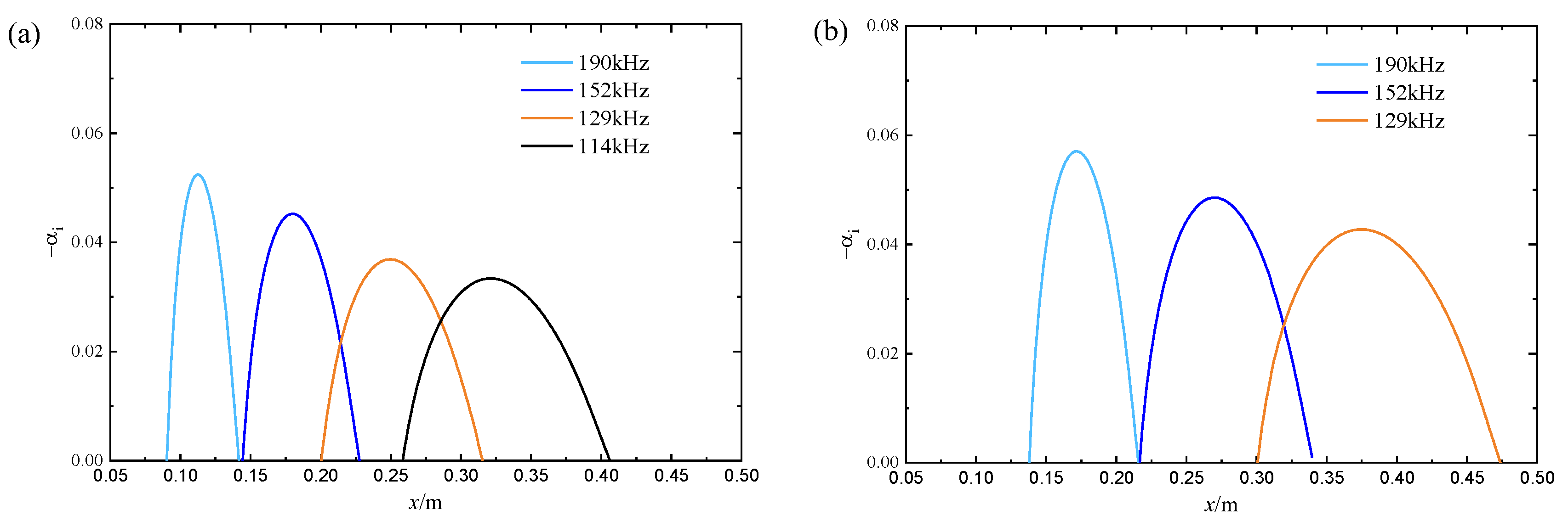
The inhouse LST code written by FORTRAN used in this paper is shown in reference [34]. Figure 8 illustrates the variations in disturbance growth rates within the ω-β plane at Rex = 6.5 × 10⁵ under the freestream conditions of case 3. Two distinct modes coexist in the boundary layer—the lower frequency corresponds to the first mode, while the higher frequency characterizes the second mode. Notably, the bandwidth of the first mode surpasses that of the second mode. The diagram emphasizes the prevalence of the second mode in the hypersonic boundary layer, notably featuring a predominantly two-dimensional disturbance. Conversely, the first mode, exhibiting the highest amplification, predominantly occurs near β = 0.8, signifying its three-dimensional perturbation nature.
The evolution of instability waves along the streamwise direction was obtained and analyzed. Figure 9 shows the PSDs of the boundary layer instability waves at several streamwise positions under different unit Reynolds numbers by PCB.
As illustrated in Figure 9, for a unit Reynolds number (Reunit) of 6.38 × 10⁶, the absence of a discernible peak characterizing second-mode waves in the power spectral density (PSD) before the streamwise location of x = 180 mm indicates that second-mode disturbances have not yet developed, signifying a laminar boundary layer state at this location. However, a subtle peak with broadband characteristics around 100 kHz emerges in the PSD at x = 240 mm, suggesting the initiation and growth of second-mode waves. Subsequently, the PSD of the second mode remains consistent between x = 330 mm and x = 360 mm, indicating saturation of the second-mode disturbances. In the case of a higher unit Reynolds number, i.e., Reunit = 8.20 × 10⁶, the peak in the PSD at the streamwise location of x = 240 mm surpasses that of Reunit = 6.38 × 10⁶, indicating the earlier appearance and growth of second-mode disturbances before x = 240 mm. Beyond x = 330 mm, the energy associated with second-mode waves exhibits a gradual increase and disperses into neighboring frequency domains, signaling the imminent breakdown of second-mode waves and the transition of the boundary layer.
According to previous studies, when the Ma > 4, the second-mode wave is more unstable, always leading to transition. Figure 10 shows the evolution of the growth rate of second-mode disturbances in different frequencies along the flow direction by LST. The second modes at different frequencies start to grow from different stations, and the high-frequency modes usually begin to arise and grow at first. Figure 10b indicates that, at the same unit Reynolds number condition, the higher frequency of the second mode wave can achieve a higher growth rate than that at low frequency. However, due to the attenuation of the high-frequency disturbance, it develops to a very short distance in the direction of flow, as shown in Figure 11. As the high-frequency modes begin to decay, the low-frequency modes in the boundary layer begin to appear and grow along the flow direction. Although the growth rate of lower-frequency disturbance is smaller than that of higher frequency, it usually becomes key to promote transition because of its larger propagation distance in the boundary layer.
As is shown in Figure 10, with the increase in the unit Reynolds number, the initial position of disturbance growth at the same frequency gradually moves backward. Under the condition of Reunit = 2.52 × 10⁶ (Figure 10a), the second mode of 190 kHz in the boundary layer decreases. Moreover, the growth rate of the disturbance is higher than that in the case of a low unit Reynolds number and moves further forward.

3.3. eN Method

The distribution of N-factor of a range of representative frequency disturbances along the flow direction is shown in Figure 11. The N-factor is sensitive to frequency and freestream unit Reynolds number. Because of the larger propagation distance in the boundary layer of relatively low-frequency disturbance, it is easier to reach a larger N- factor, as suggested in Figure 10. Because the transition position of the plate in the experiment is obviously “wavy”, the transition position calculated by the transition model γ-Reθt is used as the “average” transition position of the flat plate in the experiment. The red dashed line in Figure 10 represents the transition position obtained from the heat flow in the experiment. The N-factors of the transition location of two cases of unit Reynolds numbers are 0.98 and 1.25, respectively. Figure 12 illustrates the eigenfunction of two cases with different unit Reynolds numbers at x = 130 mm. There is no significant difference between the shape function of flow velocity u and temperature under the two experiments conditions. The normal distance of disturbance decreases with the increase in the unit Reynolds number.

4. Discussion

This study systematically examined the instability characteristics of the hypersonic boundary layer over a flat plate at a zero angle of attack, employing a combined approach of experimental analysis and linear stability analysis. The compression modification formula was fitted using the modified γ-Reθt model and the experimental results of the flat plate in a hypersonic wind tunnel. The validation results show that the predictions of the modified γ-Reθt model are more in line with the experimental results, which verifies the correctness of the modified γ-Reθt model. The application of PCB technology and infrared thermography facilitated the characterization of instability waves and enabled the calculation of the Stanton number along the streamwise direction. Additionally, the eN method was implemented to determine the N-factor at the transition location within the wind tunnel. The conclusions derived from this study are outlined as follows:
(1)
The transition model based on compressibility correction can better predict the transition position of the hypersonic boundary layer, and the simulation results are in good agreement with the experimental results. Moreover, the freestream unit Reynolds number has a great effect of the transition Reynolds number of the flat-plate boundary layer. As the unit Reynolds number increases, the transition position moves forward, and the transition Reynolds number also increases;
(2)
The LST results show that the first mode and the second mode are both present in the hypersonic boundary layer at the Mach number 5. Combined with the PCB results of the experiments, the second-mode frequency range predicted by the LST matches the frequencies measured in the experiments, with a second-mode frequency range from 100 to 250 kHz;
(3)
The N-factor of wind tunnel transition location predicted by LST is about 0.98 and 1.25 for Reunit = 6.38 × 10⁶ and 8.20 × 10⁶, respectively. With the increase in the unit Reynolds number, although the transition position moves forward, the N- factor of the transition position increases due to the increase in the magnification of the disturbance.

Author Contributions

Conceptualization, H.D.; validation, S.L.; formal analysis, Y.J.; investigation, S.L.; data curation, Y.J.; writing—original draft, Y.Y.; funding acquisition, H.D. All authors have read and agreed to the published version of the manuscript.

Funding

This research was funded by the National Numerical Wind-Tunnel (No. 2021-ZTNNW-QT00-50042, No. 2020-DY01-001), the National Natural Science Foundation of China (No. 11872208).

Institutional Review Board Statement

Not applicable.

Informed Consent Statement

Not applicable.

Data Availability Statement

Data is contained within the article.

Conflicts of Interest

The authors declare no conflict of interest.

Abbreviations

fFrequency
MaMach number
PrPrantl number
pPressure
ReReynolds number
uVelocity
TTemperature
ρDensity
x, y, zCartesian coordinates
qHeat flux
StStanton number
LSTLiner stability theory
αStreamwise wave number
−αiSpatial amplification rate
γRatio of specific heat
ωAngular frequency
βSpanwise wave number
CpSpecific heat capacity
T0Stationary temperature
T∞Freestream temperature
U∞Freestream velocity
ρ∞Freestream density
kHeat conductivity
PEEKPoly-ether-ether-ketone

References

  1. Marineau, E.C.; Grossir, G.; Wagner, A.; Leinemann, M.; Radespiel, R.; Tanno, H.; Chynoweth, B.C.; Schneider, S.P.; Wagnild, R.M.; Casper, K.M. Analysis of second-mode amplitudes on sharp cones in hypersonic wind tunnels. J. Spacecr. Rocket. 2019, 56, 307–318. [Google Scholar] [CrossRef]
  2. Jianqiang, C.; Guohua, T.; Yifeng, Z.; Guoliang, X.U.; Xianxu, Y.; Cheng, C. Hypersonic boundary layer transition: What we know where shall we go. Acta Aerodyn. A Sin. 2017, 35, 311–337. [Google Scholar]
  3. Quintanilha, H.; Paredes, P.; Hanifi, A.; Theofilis, V. Transient growth analysis of hypersonic flow over an elliptic cone. J. Fluid Mech. 2022, 935, A40. [Google Scholar] [CrossRef]
  4. Mack, L.M. Boundary-Layer Linear Stability Theory; California Inst of Tech Pasadena Jet Propulsion Lab: Pasadena, CA, USA, 1984. [Google Scholar]
  5. Mack, L.M. Linear stability theory and the problem of supersonic boundary-layer transition. AIAA J. 1975, 13, 278–289. [Google Scholar] [CrossRef]
  6. Laurence, S.J.; Wagner, A.; Hannemann, K. Experimental study of second-mode instability growth and breakdown in a hy-personic boundary layer using high-speed schlieren visualization. J. Fluid Mech. 2016, 797, 471–503. [Google Scholar] [CrossRef]
  7. Estorf, M.; Radespiel, R.; Schneider, S.; Johnson, H.; Hein, S. Surface-pressure measurements of second-mode instability in quiet hypersonic flow. In Proceedings of the 46th AIAA Aerospace Sciences Meeting and Exhibit, Reno, NV, USA, 7–10 January 2008; p. 1153. [Google Scholar]
  8. Wendt, V.; Simen, M.; Hanifi, A. An experimental and theoretical investigation of instabilities in hypersonic flat plate boundary layer flow. Phys. Fluids 1995, 7, 877–887. [Google Scholar] [CrossRef]
  9. Zhao, J.S.; Liu, S.; Zhao, L.; Zhang, Z. Numerical study of total temperature effect on hypersonic boundary layer transition. Phys. Fluids 2019, 31, 114105. [Google Scholar] [CrossRef]
  10. Zhang, C.; Shi, Z. Nonlinear wave interactions in a transitional hypersonic boundary layer. Phys. Fluids 2022, 34, 114106. [Google Scholar] [CrossRef]
  11. Cheng, J.; Huang, R.; Liu, W.; Wu, J. Influence of Single Roughness Element on Hypersonic Boundary-Layer Transition of Cone. AIAA J. 2023, 61, 3210–3218. [Google Scholar] [CrossRef]
  12. Thele, M.; Selcan, C.; Sander, T.; Rödiger, T.; Mundt, C. Bluntness-Dependent Hypersonic Boundary-Layer Modes’ Excitation. J. Spacecr. Rocket. 2022, 59, 1613–1622. [Google Scholar] [CrossRef]
  13. Borg, M.P.; Kimmel, R.L. Ground test of transition for HIFiRE-5b at flight-relevant attitudes. J. Spacecr. Rocket. 2018, 55, 1329–1340. [Google Scholar] [CrossRef]
  14. Yao, S.; Duan, Y.; Yang, P.; Wang, L.; Zhao, X.; Min, C. Experimental study of hypersonic boundary layer transition on a flat plate delta wing. Exp. Therm. Fluid Sci. 2020, 112, 109990. [Google Scholar] [CrossRef]
  15. Xu, X.; Yi, S.; Han, J.; Quan, P.; Zheng, W. Effects of steps on the hypersonic boundary layer transition over a cone at 10° angle-of-attack. Phys. Fluids 2022, 34, 034114. [Google Scholar] [CrossRef]
  16. Zhu, Y.; Zhang, C.; Chen, X.; Yuan, H.; Wu, J.; Chen, S.; Lee, C.; Gad-El-Hak, M. Transition in hypersonic boundary layers: Role of dilatational waves. AIAA J. 2016, 54, 3039–3049. [Google Scholar] [CrossRef]
  17. Liu, S.; Wang, M.; Dong, H.; Xia, T.; Chen, L.; Zhao, A. Infrared thermography of hypersonic boundary layer transition induced by isolated roughness elements. Mod. Phys. Lett. B 2021, 35, 2150500. [Google Scholar] [CrossRef]
  18. Nakagawa, K.; Tsukahara, T.; Ishida, T. DNS Study on Turbulent Transition Induced by an Interaction between Freestream Turbulence and Cylindrical Roughness in Swept Flat-Plate Boundary Layer. Aerospace 2023, 10, 128. [Google Scholar] [CrossRef]
  19. Zhou, T.; Liu, Z.; Lu, Y.; Wang, Y.; Yan, C. Direct numerical simulation of complete transition to turbulence via first-and second-mode oblique breakdown at a high-speed boundary layer. Phys. Fluids 2022, 34, 074101. [Google Scholar] [CrossRef]
  20. Saric, W.; Reshotko, E.; Arnal, D. Hypersonic Laminar-Turbulent Transition; AR-3l9; AGARD: Seine, France, 1998. [Google Scholar]
  21. Mason, W.H. Fundamental Issues in Subsonic/Transonic Expansion Corner Aerodynamics; AIAA Paper; American Institute of Aeronautics and Astronautics: Reston, VA, USA, 1993; p. 0649. [Google Scholar]
  22. Chen, F.J.; Malik, M.R.; Beckwith, I.E. Boundary-layer transition on a cone and flat plate at mach 3.5. AIAA J. 1989, 27, 687–693. [Google Scholar] [CrossRef]
  23. Juliano, T.J.; Paquin, L.; Borg, M.P. Measurement of HIFiRE-5 boundary-layer transition in a Mach-6 quiet tunnel with infrared thermograph. In Proceedings of the 54th AIAA Aerospace Sciences Meeting, San Diego, CA, USA, 4–8 January 2016; p. 0595. [Google Scholar]
  24. Tao, S.; Su, C.; Huang, Z. Improvement of the e N method for predicting hypersonic boundary-layer transition in case of modal exchange. Acta Mech. Sin. 2023, 39, 122416. [Google Scholar] [CrossRef]
  25. Zhu, W.; Shi, M.; Zhu, Y.; Lee, C. Experimental study of hypersonic boundary layer transition on a permeable wall of a flared cone. Phys. Fluids 2020, 32, 011701. [Google Scholar] [CrossRef]
  26. Chen, X.L.; Fu, S. Linear stability analysis of hypersonic boundary layer on a flat-plate with thermal-chemical non-equilibrium effects. Acta Aerodyn. Sin. 2020, 38, 316–325. [Google Scholar]
  27. Klothakis, A.; Quintanilha Jr, H.; Sawant, S.S.; Protopapadakis, E.; Theofilis, V.; Levin, D.A. Linear stability analysis of hypersonic boundary layers computed by a kinetic approach: A semi-infinite flat plate at 4.5 ≤ M∞ ≤ 9. Theor. Comput. Fluid Dyn. 2022, 36, 117–139. [Google Scholar] [CrossRef]
  28. Boyd, C.F.; Howell, A. Numerical Investigation of One-Dimensional Heat-Flux Calculations; Technical Report NSWCDD/TR-94/114; Dahlgren Division Naval Surface Warfare Center: Silver Spring, MD, USA, 1994. [Google Scholar]
  29. Menter, F.R. Two-equation eddy-viscosity turbulence models for engineering applications. AIAA J. 1994, 32, 1598–1605. [Google Scholar] [CrossRef]
  30. Chedevergne, F. A double-averaged Navier-Stokes k–ω turbulence model for wall flows over rough surfaces with heat transfer. J. Turbul. 2021, 22, 713–734. [Google Scholar] [CrossRef]
  31. White, F.M. Viscous Fluid Flow, 3rd ed.; McGraw-Hill Series in Mechanical Engineering; McGraw-Hill Higher Education: New York, NY, USA, 2006. [Google Scholar]
  32. Willems, S.; Gülhan, A.; Steelant, J. Experiments on the effect of laminar–turbulent transition on the SWBLI in H2K at Mach 6. Exp. Fluids 2015, 56, 49. [Google Scholar] [CrossRef]
  33. Menter, F.R.; Langtry, R.B.; Likki, S.R.; Suzen, Y.B.; Huang, P.G.; Völker, S. A correlation-based transition model using local variables—Part I: Model formulation. J. Turbomach. 2006, 128, 413–422. [Google Scholar] [CrossRef]
  34. Guo, X.; Tang, D.; Shen, Q. Boundary layer stability with multiple modes in hypersonic flows. Mod. Phys. Lett. B 2009, 23, 321–324. [Google Scholar] [CrossRef]
Figure 1. Sketch of NHW wind tunnel.
Applsci 13 13302 g001
Figure 2. Schematic diagram of flat-plate installation in wind tunnel.
Applsci 13 13302 g002
Figure 3. Schematic diagram of flat-plate mesh division and boundary conditions.
Applsci 13 13302 g003
Figure 4. Comparation of mean flow variables at x = 0.1 m.
Applsci 13 13302 g004
Figure 5. Surface temperature distribution of a flat plate under different unit Reynolds numbers: (a) Reunit = 2.56 × 10⁶; (b) Reunit = 6.38 × 10⁶; (c) Reunit = 8.20 × 10⁶.
Applsci 13 13302 g005
Figure 6. Mean Stanton number distribution of plate flow direction under different unit Reynolds numbers: (a) Reunit = 2.56 × 10⁶; (b) Reunit = 6.38 × 10⁶; (c) Reunit = 8.20 × 10⁶.
Applsci 13 13302 g006
Figure 7. Transition Reynolds number distribution of plate spanwise at different unit Reynolds numbers: (a) Reunit = 2.56 × 10⁶; (b) Reunit = 6.38 × 10⁶; (c) Reunit = 8.20 × 10⁶.
Applsci 13 13302 g007
Figure 8. Growth rate in ω-β plane: (a) Reunit = 6.38 × 10⁶; (b) Reunit = 8.20 × 10⁶.
Applsci 13 13302 g008
Figure 9. Comparison of PCB-measured spectra along the streamwise direction: (a) Reunit = 6.38 × 10⁶; (b) Reunit = 8.20 × 10⁶.
Applsci 13 13302 g009
Figure 10. The growth rate of second-mode waves along flow directions predicted by LST: (a) Reunit = 6.38 × 10⁶; (b) Reunit = 8.20 × 10⁶.
Applsci 13 13302 g010
Figure 11. N-factor predicted by LST: (a) Reunit = 6.38 × 10⁶; (b) Reunit = 8.20 × 10⁶.
Applsci 13 13302 g011
Figure 12. Eigenfunction predicted by LST at x = 130 mm. (a) xxx Eigenfunction of stream-wise velocity (b) Eigenfunction of Temperature.
Applsci 13 13302 g012
Table 1. Flow condition.
Flow ConditionP0/kPaT0/KRe/m/106
Ma = 5Case1200.15012.52
Case2490.54916.38
Case3729.95398.20
Disclaimer/Publisher’s Note: The statements, opinions and data contained in all publications are solely those of the individual author(s) and contributor(s) and not of MDPI and/or the editor(s). MDPI and/or the editor(s) disclaim responsibility for any injury to people or property resulting from any ideas, methods, instructions or products referred to in the content.

