Abstract
CCTVs are commonly used for traffic monitoring and accident detection, but their images suffer from severe perspective distortion causing object size reduction with distance. This issue is exacerbated in tunnel CCTVs, positioned low due to space constraints, leading to challenging object detection, especially for distant small objects, due to perspective effects. To address this, this study proposes a solution involving a region of interest setup and an inverse perspective transformation technique. The transformed images, achieved through this technique, enlarge distant objects, maintaining object detection performance and appearance velocity across distances. To validate this, artificial CCTV images were generated in a virtual tunnel environment, creating original and transformed image datasets under identical conditions. Comparisons were made between the appearance velocity and object size of individual vehicles and for deep learning model performance with multiple moving vehicles. The evaluation was conducted across four distance intervals (50 m to 200 m) from the tunnel CCTV location. The results reveal that the model using original images experiences a significant decline in object detection performance beyond 100 m, while the transformed image-based model maintains a consistent performance up to the distance of 200 m.
1. Introduction
Video surveillance systems are broadly used in many countries to monitor traffic volume and to detect accidents at an early stage to prevent secondary accidents [1,2,3]. Typically, these accidents involve vehicles or pedestrians on the road, making it essential to implement early object detection systems based on CCTVs. This requirement is mandatory in most countries. Based on the detected object information, it becomes possible to develop evaluation algorithms or accident response processes for CCTV surveillance systems. For this purpose, a number of studies have been conducted in various academic fields, such as emergency transportation methods [4], road vehicle accident responses [5], railway crossing surveillance [6], and monitoring systems of construction vehicles at construction sites [7,8].
In tunnels, there is a much higher probability of road traffic accidents in entering or exiting zones because of illumination changes which sometimes cause temporary light or dark adaptations to drivers [9,10,11,12]. Additionally, evacuation areas are often limited in the tunnels, and this may lead to severe secondary accidents. To minimize those accidents in such environments, it is crucial to promptly detect and respond to the accidents via video surveillance systems. CCTVs in the tunnels are normally installed at lower positions compared to those on open roads, as illustrated in Figure 1. Therefore, these CCTV installations lead to severely distorted perspective footage, and this image distortion causes poor recognition of vehicles or humans as the relative distance between the CCTVs and the identified objects increases [13]. In particular, this mechanism has disadvantages in object detection (OD) performance using computer vision techniques [14].
Figure 1 shows the captured images from two different CCTVs on a highway and a tunnel, demonstrating the effect of installation height on perspective and overlap. In an open road site, First, as shown in Figure 1a, the CCTV can be installed at a height of at least 8 m or higher, as there are no space constraints in the vertical direction. Consequently, the perspective effect is less pronounced, as in Figure 1a. In addition, the lane width is represented by white straight lines, at the end of a distance of about 100 m. The lane width at the far side appears to be approximately 0.5 times smaller than the one at the near side. On the other hand, in the tunnel CCTV (Figure 1b), the lane width at the far side appears to be 0.09 times smaller than the one at 100 m away, indicating a more severe perspective effect compared to Figure 1a [15].

Figure 1.
Comparison of CCTV images based on installation height: (a) CCTV for open roads [16]; (b) tunnel CCTV.
In addition, there is a significant difference in the overlapping of vehicles depending on the CCTV installation height. The higher the CCTV installation height, the closer it is to the top-view image. Therefore, in situations with numerous vehicles in traffic (Figure 1a), only a portion of them overlap, allowing for a better distinction of each vehicle, as seen in the actual road image in Figure 1a. In contrast, as illustrated in Figure 1b, vehicles that are distinct from the CCTV appear to be heavily overlapped, which could potentially obstruct the visibility of rear vehicles.
To address the issue of decreased OD performance due to perspective, Min et al. conducted a study aiming to improve the OD performance for detecting persons in tunnel CCTV images using high-resolution reconstruction [17]. Min et al. [17] reported a 2% improvement in the OD performance for detecting persons, increasing from 88% to 90%. However, Min. et al. [17] did not address any geometrical effect of the high perspective phenomenon which, we believe, might be more sensitive in OD performance than the resolution of CCTV in tunnel environment.
In fact, OD performance in tunnel sites has not been addressed to date, even if a traffic accident in a tunnel causes highly risky secondary accidents with expected low OD performance in a highly disadvantageous tunnel CCTV environment. Therefore, this study demonstrates the difficulties in the aspect of tunnel environment, and is focused on the high-perspective effect due to low CCTV installation. Then, an attempt is made to overcome it by introducing an inverse perspective transform (IPT) technique with some experimental evidence, aiming to achieve size uniformity between distant and close objects. Experiments were conducted on the tunnel CCTV images, which were chosen due to their higher susceptibility to perspective effect compared to open road site images. Furthermore, to exclude other influencing factors aside from the perspective effect in OD on images, a virtual tunnel environment was utilized. Various moving vehicles were generated within the virtual tunnel, and CCTV images were artificially produced using game development software called ‘UNITY (2019.3.9f1)’ instead of using actual tunnel site images. Based on this, a virtual tunnel and moving vehicle video dataset were created, and a deep learning model was built. Subsequently, the effectiveness of the introduced IPT technique was objectively accessed through the review of the appearance characteristic (AC) of vehicle objects and the training experiment of the deep learning model. A study was then conducted to quantitatively identify the improvement effect on OD performance resulting from the application of the IPT technique.
2. Inverse Perspective Transform (IPT)
2.1. Concept and Application of IPT
In this study, the introduced technique referred to as IPT involves the geometric transformation [18] of an image by modifying the arrangement structure of pixels based on a principle. The IPT technique represents one of the image transformation methods primarily employed to correct and mitigate perspective issues within a given image [19,20,21,22]. As mentioned in the introduction, IPT has found applications in various fields.
In the field of autonomous driving, a number of studies have been conducted utilizing IPT to identify lane information through lane detection [23,24] and road sign detection [25] from images acquired after applying the IPT technique. Furthermore, in various domains, IPT has been employed for generating top-view images from rearview cameras during parking maneuvers [26], road orthophoto mapping [27], and real-time detection of cut-in violation vehicles based on CCTV [28]. It is noted that in this general autonomous driving area, imaging points are moving with the vehicle body, the and target distance of concern is relatively near to the points.
Apart from the concern above, this study is focused on tunnel environments where any imaging points (CCTV) are fixed at law height and law brightness, and any incident for detection can take place at any distance from the points.
2.2. Setting of a Region of Interest (ROI) for IPT
This paper focuses on applying the IPT technique to the tunnel CCTV image, referred to as the original image (OI), and this involves the initial establishment of a region of interest (ROI) [29]. The ROI is defined as a quadrangular shape, conforming to the road width and CCTV installation spacing when the image is stretched and observed on a horizontal plane, as illustrated in Figure 2a [29]. In this context, Figure 2b serves as an OI coordinate system, its origin is at the top left corner, the rightward horizontal direction is denoted as the x axis, and the downward vertical direction is denoted as the y axis. Subsequently, upon transforming Figure 2b into a horizontal plane image, the term transformed image (TI) is introduced, with its origin located at the top left corner, as depicted in Figure 2a. The TI coordinate system is defined, with the x’ axis indicating the rightward horizontal direction and the y’ axis indicating the downward vertical direction. To generate the TI as shown in Figure 2a, the ROI must first be designated on the OI in Figure 2b by following the prescribed procedure described in Figure 3.
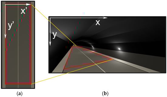
Figure 2.
ROI configuration in a tunnel CCTV image: (a) top-view image; (b) tunnel CCTV image.
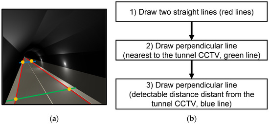
Figure 3.
The procedure of finding four ROI points: (a) finding the four ROI points (yellow points) in a tunnel CCTV image and (b) flow chart.
Figure 3 shows the procedure for finding four points of interest for setting ROI for tunnel CCTV as a figure (Figure 3a) and a flow chart (Figure 3b). In Figure 3b, each process is described in detail as follows:
(1) In the world coordinate system, the two red lines are parallel to the vehicle’s driving direction, and are located at the edge of the road.
(2,3) Green and blue lines are drawn which are perpendicular to (nearest between) the lines drawn in (1) in the world coordinate system.
Through this process, the four orange points are found which the intersection of each of the lines, as shown in Figure 3a, and these points are used to define ROI. Using the coordinates of these four vertices of the ROI, an image conversion is conducted to transition from OI to a horizontal plane. The ROI, once converted to the horizontal plane image, takes the form of a rectangle.
2.3. IPT Procedures
Subsequently, to execute IPT, a Homography matrix is required to embody the relational transformation of coordinates between corresponding points within both the OI and horizontal plane converted images [30]. Given a point (x,y) in the OI coordinate system and a point (x’,y’) in the TI coordinate system, a geometric coordinate transformation from an arbitrary quadrangular ROI to a rectangle is undertaken by the following Equation (1).
In Equation (1), S is a scale factor which is required to scale between the two coordinate systems on OI and TI, respectively, and H represents the matrix in the form of a 3 × 3 matrix. In this context, matrix H is derivable by computer algorithms [31]. The of the matrix H is normalized to 1 due to the homogeneity of the TI coordinates incorporating the scale factor S. With regard to other parameters, govern rotation, scale, shearing and reflection, respectively, whereas regulate translation and underpin perspective transformation.
A more detailed depiction of this IPT process is shown in Figure 4. First, the matrix between the blue rectangular box and the prescribed red ROI in Figure 4a is established. Then, the IPT with the composed matrix is applied to the cropped red ROI on OI, consequently resulting in the TI, as shown in Figure 4b. Through this process, the point (x,y) in the OI coordinate system shown in Figure 4a is at the same location as the point (x′,y′) in the TI coordinate system shown in Figure 4b. The TI derived from this elaborate procedure guarantees a relatively constant object size regardless of the distance from the tunnel CCTV, thereby preserving the calculated vehicle object’s velocity from the TI at an approximate constancy. Nonetheless, as IPT constitutes a geometric transformation, objects positioned farther from the tunnel’s CCTV experience a reduction in their inherent resolution, resulting from their elongation.
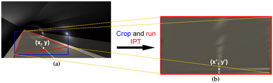
Figure 4.
The process of obtaining a TI-based on ROI in a tunnel CCTV image: (a) tunnel CCTV image with ROI, (b) transformed image.
3. Generation of a Virtual Video and Appearance Attributes of the Moving Vehicles
3.1. Backgrounds
The visible attributes of perspective are addressed to demonstrate the viability of introducing IPT. However, to execute an empirical inquiry in real tunnel CCTV environments, the acquisition of distance and vehicle position data pertinent to authentic road tunnel locations becomes essential. The accurate measurement on the road tunnels presents challenges due to the presence of other vehicles in motion, exacerbated by the inherent variability in the driving velocities of these vehicles within the environment. As a result, this study adopts an approach involving the creation of a virtual tunnel, accomplished via the utilization of the UNITY engine game development platform [32]. Through the virtual tunnel image model, essential information encompassing individual object attributes, spatial positioning, and velocity attributes of diverse vehicles situated within the tunnel milieu are derived. Predicated upon these synthetically generated images and corresponding vehicular positional data, this investigation scrutinizes the appearance attributes of the moving vehicles inherent to perspective within tunnel CCTV.
3.2. Generation of a Virtual CCTV Video
The WCS and OI coordinate system on the image plane of tunnel CCTV are depicted in Figure 5. In the WCS, the tunnel CCTV image is taken at the point ‘O’ which is the location of a CCTV installation. The WCS is represented by X, Y and Z, and the vehicle’s movement on the ground plane is directed into the negative Z axis. The vertical dimension corresponds to the Y axis, while the lateral directions are aligned with the X axis. On the other hand, the image plane on the CCTV is represented in the two-dimensional OI coordinate system on which the horizontal and vertical directions are denoted by x axis and the y axis, respectively. In this context, the virtual tunnel is conceptualized as a straight, one-way, two-lane tunnel with a width of 12.6 m, a height of 6.2 m and a length of 5 km. Additionally, virtual tunnels were created in a straight tunnel by using a collection of modeled road data called the Low Poly Road Pack [33].
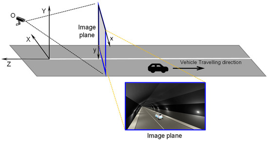
Figure 5.
WCS and OI coordinate system in a 3D virtual tunnel site.
Based on the WCS, the specification of the virtual CCTV installation specification is outlined in Table 1. The CCTV is located at the height of 11 m along the Z axis. Regarding the CCTV rotation angles, α, β, and γ, these correspond, respectively, to rotations around the X, Y, and Z axis. The selected rotation angles are calibrated to achieve a resemblance with the actual tunnel image in Figure 1b.

Table 1.
Specification of the virtual tunnel CCTV.
This study involves the creation of two distinct videos. The creation of the two videos is achieved through the Recorder Window, which is one of UNITY’s plugins, and the video is created and saved by the installed CCTV in CCTV viewing direction. The first video portrays a single vehicle in motion, aiming to identify the appearance velocity (AV) and changes in the viewing size attributed to the vehicle objects on the image plane. The second video depicts multiple vehicles in motion, undertaken to facilitate a comparative analysis of the OD performance through the use of deep learning models. Initially, the single vehicle motion video features a vehicle traveling at a constant speed of 100 km/h. This vehicle possesses dimensions resembling those of a standard passenger car, being 4.2 m in length, 2.2 m in width, and 1.4 m in height. This vehicle, as well as the vehicles in the multi-vehicle motion video described below, utilized Low Poly Cars [34], which is a collection of pre-modeled vehicle data.
Conversely, for the multi-vehicle motion video, nine vehicles are incorporated, consisting of one bus, two trucks and six passenger cars, all maintaining a constant velocity. Detailed specifications for this video are presented in Table 2. The video resolution is specified in Table 2, and is characterized by dimensions W (width) and H (height).
Table 2.
Composition of video data.
The specifications for each vehicle object are shown in Table A1 of Appendix A and are modeled to resemble real-world vehicles; we intended to avoid any influencing factors other than the vehicle viewing distance. Furthermore, the shape of each object can be seen in Figure A1, and utilizes different colors. For the multi-vehicle video scenario, all vehicles are basically driving at a constant speed. Then, as shown in Figure A2, there are three patterns in a single video, which appear within a time interval of about 3 s. The speeds of the vehicles in each pattern are set up as shown in Figure A2a–c to create a realistic traffic flow.
3.3. Composition of Image Datasets for IPT
To investigate the perspective relaxation in tunnel CCTV images, it is necessary that the comparative conditions of OI and TI remain identical. Therefore, parity is maintained in terms of absolute area and dimensions for each ROI across both images, and the spatial range of ROIs aligned with the direction of vehicle movement within the tunnel is uniformly set to 200 m for both OI and TI, which reflects the standard installation distance for tunnels in the South Korea, as shown in Figure 6. In order to compose two cases of image datasets with ensuring uniformity in comparative conditions, the following processes are undertaken: for the first case of dataset, the background outside the designated ROI on OI is removed to be black, followed by subsequent cropping of the blue box area as illustrated in Figure 6a. This cropped image dataset is denominated as ORG in Figure 6a. Then, for composing the next case of dataset, using the composed Homography matrix between the cropped blue box and the ROI region in red, the ORG dataset is transformed by IPT with the matrix, followed by second cropping of the red ROI region to obtain the transformed dataset TRANS, as shown in Figure 6b.
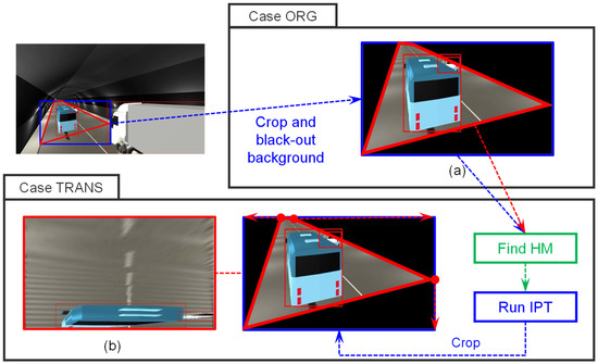
Figure 6.
Composition of comparative datasets through IPT processes: (a) case ORG (b) case TRANS.
3.4. Comparison of AC for Single-Vehicle
Based on the two distinct datasets, AC with a single vehicle object is investigated with a comparison of the AV of the vehicle on both datasets. The specified vehicle object undertakes uniform motion at a constant velocity of 100 km/h, progressing in the the -Z direction. Then, a script on the UNITY engine was created to save the actual location of the vehicle in world coordinate system, the location of the vehicle on the video, and the object information at a certain time, which was obtained in the run of the UNITY engine. All the information wase saved in a file and then used for analyzing the ACs in this section. A comparison of ACs for the actual trajectory of the vehicle object in OI and TI coordinate systems is presented in Figure 7.
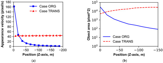
Figure 7.
Comparison of (a) AV, and (b) object area between case ORG and case TRANS.
The genuine trajectory of the vehicle aligns with the −Z direction in WCS. The computation of AV, however, is conducted in the −y direction within the image plane of Figure 5. The movements of the vehicle on ORG and TRANS are determined in the image plane of CCTV, as shown in Figure 6. Additionally, the bounding box of the vehicle is drawn, and the movement of the base line of the box is harnessed for calculating AV, utilizing pixel values along the vertical axis. The variation in pixel values, termed “dy” along with the defined time interval “dt”, facilitates the expression of AV through the following Equation (2).
The variation in AVs computed on both image planes, ORG and TRANS, is compared in Figure 7a. The observed trend in Figure 7a illustrates a pronounced reduction in AV along the ORG as the vehicle retreats from the installation point of the CCTV. This phenomenon can be attributed to the effects of perspective, wherein the AV tends to approach a nominal value upon traversing a point of 100 m distant from the initial reference line. Conversely, the AV trend for TRANS exhibits an inclination toward constancy, regardless of vehicle location. The mitigating impact of relaxed perspective becomes evident in this context, thereby engendering minimal fluctuations in AV.
Simultaneously, the relaxation of perspective substantially affects alterations in the area of the vehicle’s bounding box in accordance with its actual position. In this case, the area of the object can be calculated as the product of the object’s width and height. Figure 7b illustrates these case-specific attributes. To avoid the impact stemming from the gradual diminution of the vehicle’s bounding box, attributable to its progressive disappearance beyond the confines of the ROIs, the calculation of the vehicle’s box area is limited to distances up to −150 m. In Figure 7b, the vehicle’s area shows a pronounced reduction in the ORG as it progressively moves away from the tunnel CCTV. Conversely, the area variation in the TRANS shows a gradual increase, albeit with a relatively smaller variance.
Collectively considering the two sets of ACs, in the case ORG, it becomes apparent that the perspective in the ORG leads to a divergence from the actual attributes of the vehicle entity. Conversely, the relaxed perspective in the TRANS engenders a noticeable alignment between the calculated AC and the intrinsic attributes of the vehicle entity.
Furthermore, the change in vehicle object area at location for each case can be seen visually in Figure A3 of Appendix A. In Figure A3, the shape of the object is preserved in the distance for the case ORG, but their sizes are sharply reduced upon moving away, due to the perspective effect. On the other hand, in case TRANS, the shape of the object is gradually elongated vertically by moving from 0 m to −150 m, and the height of the object gradually increases, while the width of the object remains almost unchanged. Based on this viewing phenomenon, the impact of object size changes on the performance of deep learning-based OD models are quantitatively examined in this study.
4. Comparative Experiment on Deep Learning Model Performance
In this section, the OD performance is investigated for both the ORG and TRANS image datasets with discrete distance segments. This comparative experiment is facilitated through the deployment of a convolutional neural network (CNN)-based deep learning model [35,36,37,38,39].
As usual, it is important to recognize that the efficacy of a deep learning model is intricately influenced by the dimensions of the object under consideration. Smaller object sizes cause difficulty during both the training and inference processes, primarily due to the intricate nature of extracting a pertinent feature map for such objects [40,41,42].
To investigate this aspect in the tunnel, two image datasets derived from multi-vehicles video are employed: ORG on OI and TRANS on TI. It is obvious that inconsistency in OD performance of the moving vehicles in the distance leads to instability in the detection of phenomena such as backward-travelling or stopping vehicles in the tunnel.
4.1. Preparation of Training Dataset
In the process of training our model, the datasets corresponding to vehicle objects in the ORG and TRANS were meticulously annotated. These datasets are derived from the same multi-vehicle video. Consequently, both datasets encompass an identical count of images and objects. Furthermore, the resolution of these image datasets has been standardized to 646 × 324 pixels, which is a resolution inferior to that of the original video image. A comprehensive overview of the labeled data composition is presented in Table 3. As listed in Table 3, the number of images is divided into a ratio of 8:2 for training and testing subsets. It is imperative to note that the testing dataset remains untrained during the whole training phase. Furthermore, the training dataset is further partitioned into a ratio of 8:2, creating pre-training and validation subsets. The pre-training dataset is used for the crucial purpose of preliminary training, which is for the calibration of deep learning hyperparameters and the training environment. In fact, the validation dataset, an offshoot of the training dataset, is not used for the pre-training, but is added to the training dataset at the stage of a subsequent primary training.
Table 3.
Composition of the labeled dataset and its subdivision for training and validation.
4.2. Configuration of Training Hyperparameters through Pre-Training
In this paper, Faster R-CNN [43] is adopted as the deep learning mode for utilization. Faster R-CNN, a product of evolutionary progression within the R-CNN family, gained substantial prominence following its release in 2015, which was attributed to its heightened ability to swiftly and accurately propose potential objects in comparison to the pre-existing Fast R-CNN [44]. This enhanced capability is attributed to the integration of a region proposal network (RPN) into the architecture. the intricate structure of Faster R-CNN reveals its underlying operational efficacy. It is noted that the adopted deep learning algorithm is not an important factor in this paper, because the algorithm is used for comparative purposes in the same training environment.
The primary input to this model comprises an image, subsequently subjected to the process of feature map extraction via CNN procedures. Within the intermediate phase of processing, the RPN takes center stage, effectively generating potential bounding boxes through a combination of objectness and regression analyses. These initially proposed bounding boxes then undergo a post-processing phase, facilitated by non-maximum suppression (NMS) [45]. Furthermore, the terminal component of the architecture, the fully connected layer (FC layer), plays a pivotal role in ascertaining the object’s categorical classification and precisely determining the coordinates of its bounding box.
Since this study considers the impact of perspective at low CCTV height, the overlapping phenomenon of many objects is highly visible. Therefore, the hyperparameters, epoch and NMS intersection-over-union (IOU) threshold, which are sensitive to it, were selected for sensitivity analysis and calibration through preliminary training. An epoch is defined as the training unit of a deep learning model, which is one epoch when the entire train dataset is trained once [46]. In general, the number of training epochs until the loss function of a deep learning model is converged should be determined in advance. The NMS IOU threshold is a hyperparameter used by the NMS module, which checks the overlap ratio between the bounding boxes to be post-processed, and removes them as duplicates when the threshold is exceeded. In this paper, NMS removes the overlapping bounding boxes for the proposals in the RPN stage. In this case, depending on the NMS IOU threshold, bounding boxes with less than 10 to 20% overlap are passed to the FC layer, or bounding boxes with more than 80 to 90% overlap are passed to the FC layer, affecting the weight update of Faster R-CNN. Other layouts of training configurations adopted in this study are summarized in Table 4.
Table 4.
Hyperparameters of Faster R-CNN.
4.3. Training Environment
The Faster R-CNN training in this paper utilized the mm detection code [49], and when resizing the proposal to be delivered to the FC layer, ROI align [50] was used instead of ROI pooling in the original paper.
The training environment for the deep learning model was Ubuntu 20.04, and the training was performed on the following hardware: Intel E5-2660V3 ×2, RAM 128 GB, NVIDIA GTX 1080 ×4. For the training platform, this paper used Python 3.7, pytorch 1.12.1, and numpy 1.21.6. The initial epoch for pre-training was set to 200. The IOU threshold for true/false determination was 0.5.
4.4. Determination of Training Epochs
The training duration for the deep learning model encompassed approximately 53 min/200 epochs for both datasets, ORG and TRANS. Throughout this training process, the values of the loss function were recorded for both the training and the validation datasets at every epoch, as shown in Figure 8 and Figure 9.
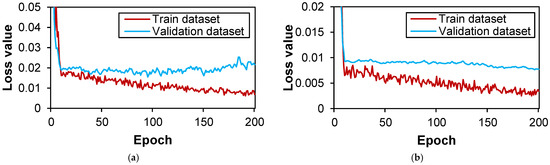
Figure 8.
Evolution of loss values over epoch in case ORG: (a) classification loss; (b) regression loss.
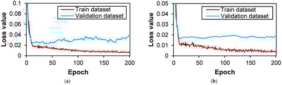
Figure 9.
Evolution of loss values over epoch in case TRANS: (a) classification loss; (b) regression loss.
Figure 8 shows the dynamic progression of the loss function across the ORG dataset. In Figure 8, it becomes evident that the classification and regression losses exhibit a tendency to converge harmoniously throughout the entirety of the epochs. However, an observation arises from the validation dataset’s loss curves, as depicted in Figure 8, revealing divergence post approximately 100 epochs in the former, and a stagnation without noticeable decline in the latter. Consequently, a selection of 100 epochs emerges as the optimal training epoch for the ORG case. The analogous approach is applied to the TRANS dataset, as depicted in Figure 9. Here, similar trends of convergence in classification and regression losses within the training dataset are apparent throughout the epochal evolution. Notably, the validation dataset’s loss curves follow a pattern similar to that observed in Figure 8, with divergence commencing around 50 epochs in Figure 9a and a sustained lack of discernible decrease in Figure 9b. Thus, a proper choice designates 50 epochs as the optimum training epoch for the TRANS case.
4.5. Determination of the NMS IOU Threshold
A sensitivity analysis with the NMS IOU threshold, which is a sensitive hyperparameter in OD tasks involving overlapped objects, is undertaken. For this purpose, a series of deep learning models are trained across a spectrum of epochs and training conditions, as ascertained in prior sections. The prescribed datasets, ORG and TRANS, are enlisted to facilitate the training procedure. Notably, six distinctive IOU threshold values (0.4, 0.5, 0.6, 0.7, 0.8, and 0.9) are selected for comprehensive analysis, and these thresholds subsequently underpin the training regime for the deep learning models. As a result, the trajectory of the loss function dynamics and the intricate interplay of average precision (AP) values are scrutinized [51], focusing on the diverse facets of the NMS IOU threshold.
Primarily, an insight into the variation of loss function reveals its profound linkage to the NMS IOU threshold. This phenomenon is graphically portrayed in Figure 10, Figure 11, Figure 12 and Figure 13, encapsulating the nuanced fluctuations across various epochs.
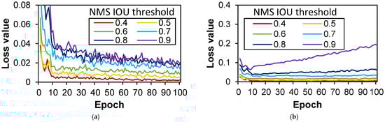
Figure 10.
Evolution of classification loss over epoch with NMS IOU thresholds in case ORG: (a) training dataset; (b) validation dataset.
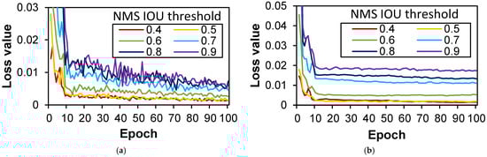
Figure 11.
Evolution of regression loss over epoch with NMS IOU thresholds in case ORG: (a) training dataset; (b) validation dataset.
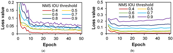
Figure 12.
Evolution of classification loss over epoch with NMS IOU thresholds in case TRANS: (a) training dataset; (b) validation dataset.
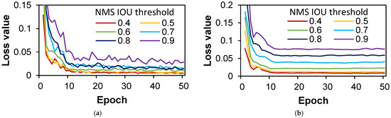
Figure 13.
Evolution of regression loss over epoch with NMS IOU thresholds in case TRANS: (a) training dataset; (b) validation dataset.
Figure 10 and Figure 11 affords a comprehensive view of the classification and regression loss trends, with emphasis on the ORG dataset. A notable observation is the discernible divergence in the validation dataset’s classification loss curve, depicted in Figure 10b, as the NMS IOU threshold escalates, attaining its zenith at a threshold value of 0.9. Similarly, the regression loss curves depicted in Figure 11b reveal elevated values for NMS IOU thresholds ranging from 0.7 to 0.9, thereby suggesting the prudent selection of thresholds between 0.4 and 0.6 based on loss metrics and their trends.
Further elaboration is carried out for the TRANS dataset, as disclosed by Figure 12 and Figure 13. The training dataset manifests convergence in all loss values, aptly depicted in Figure 12a, while the classification loss curves within the validation dataset demonstrate a proclivity for divergence at NMS IOU thresholds between 0.7 and 0.9, prompting the prudent selection of thresholds within the 0.4 to 0.6 range for the TRANS case.
Subsequently, a study of AP values at the culminating training epoch, as exhibited in Figure 14, follows the initial loss function assessment within NMS IOU thresholds ranging from 0.4 to 0.6. An assessment of AP values within this range reinforces this notion, leading to the selection of 0.6 as the optimal NMS IOU threshold for the ORG case. In concurrence, the TRANS case aligns with a comparable viewpoint, endorsing an NMS IOU threshold of 0.6. This choice is substantiated by the marginal variation in AP values within the 0.4 to 0.6 range, guided by the advantageous aspects of elevated threshold values, a principle elaborated upon in the introduction.
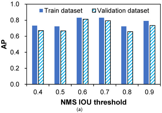
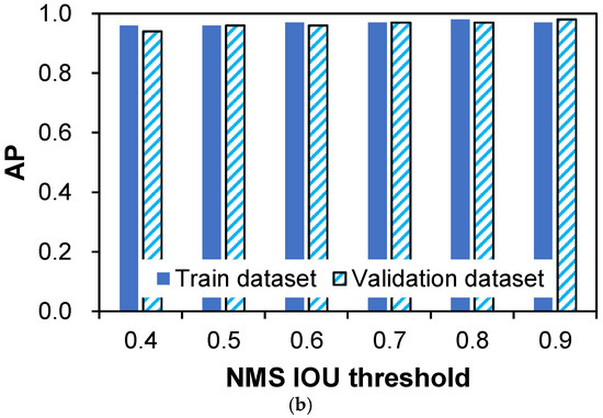
Figure 14.
AP value for trained deep learning models across NMS IOU thresholds: (a) case ORG; (b) case TRANS.
4.6. Main Training Method and Conditions
Primary training is executed using the previously determined epoch and NMS IOU threshold values. The training dataset provided in Table 3 is employed. Both cases, ORG and TRANS, contain the same number of images and vehicle objects. The ORG dataset exists in the OI coordinate system, and the TRANS case is generated by geometrically transforming ORG using IPT into the TI coordinate system. The performance of OI and TI is compared in every distance section, illustrated in Figure 15. To evaluate OD performance for each distance section, we set the ROI at 200 m (Figure 15), dividing it into four sections of 50 m intervals for AP value comparison. Vehicle objects from ORG and TRANS, the test dataset in Table 3, are allocated to corresponding sections on OI and TI based on the bounding box center point. Details of the test dataset allocation are shown in Table 5. AP value comparison is solely performed on the test dataset, adhering to the prescribed distance sections. Notably, objects in ORG and TRANS images vary in size and shape due to IPT. Thus, vehicle objects are annotated for OD for each case. Reference coordinate systems differ for both cases, causing variations in allocated sections, despite having the same object. Consequently, the number of images and vehicle objects in the prescribed sections may differ, as seen in Table 5.
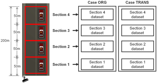
Figure 15.
Schematic diagram for division of distance sections in an image.
Table 5.
Allocation status of image and object data into distance sections.
For the primary training hyperparameters, the epochs and NMS IOU threshold determined during pre-training are employed. The remaining training parameters remain consistent with those detailed in Table 4. In this instance, case ORG has 100 epochs, case TRANS has 50 epochs, and both cases adopt an NMS IOU threshold of 0.6. Other training conditions align with those established during preliminary training.
4.7. Experiment Results
Consequently, the results of this investigation with AP values are compared for the test dataset independently across each of the four sections, as illustrated in Figure 16, and subsequently compare the absolute AP values. In Section 1, case ORG and case TRANS yield AP values of 0.985 and 0.956, respectively. While the AP value of case ORG is 0.029 higher, the absolute value itself underscores that both cases exhibit a high level of OD performance. For Section 2, case ORG and case TRANS register AP values of 0.951 and 0.917, respectively, signaling a comparable level of OD performance. Case ORG’s AP value outperforms by 0.034. In this section, both cases can be attributed to having commendable OD performance. However, within Section 3, the AP values for case ORG and case TRANS stand at 0.61 and 0.795, respectively. In comparison to Section 2, the disparity in OD performance becomes notably pronounced, driven by the AP value of case TRANS’ decreasing by 0.122, and that of case ORG decreasing by 0.341. Moving to Section 4, the contrast between case ORG and case TRANS becomes substantially more pronounced, reflecting AP values of 0.069 for case ORG and 0.952 for case TRANS. In comparison to Section 3, the AP value of case TRANS is actually enhanced by 0.157, whereas case ORG experiences a significant drop of 0.541. Given case ORG’s AP value, it becomes evident that detecting vehicles within distant Section 4 is particularly challenging due to the vehicles’ diminutive size.
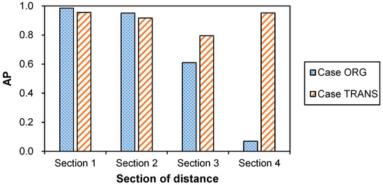
Figure 16.
Evaluation of OD performances of trained deep learning models on test dataset using AP metric for both ORG and TRANS.
4.8. Discussion
In summation, the evaluation of vehicle movement within the original image (OI) reveals a notable discrepancy between the AV and the actual velocity, coupled with a rapid diminution in object size as it recedes from the tunnel CCTV. This occurrence is predominantly attributed to a perspective effect, significantly influencing the training and inference phases of deep learning OD applications.
The reason for this can be seen in the change in the object area and shape in distance, as shown in Figure 7b and Figure A3. In Figure 7b, the object area for a single vehicle is larger than 100 pixels2 within −100 m, which can be trained and inferred by the deep learning OD model, but it shrinks rapidly beyond −100 m and becomes almost as small as a dot, as shown in Figure A3c,d. This size effect could be a major reason for poor OD performance in the −100 to −200 m range. Nevertheless, application of OI exhibits reasonable OD performance within a relatively proximate range of around 100 m.
However, OD performance experiences a marked decline beyond this 100 m threshold. Consequently, it can be deduced that OD efficacy, relying on the original CCTV image, is confined to a distance limit of 100 m within the tunnel environment. This limitation is attributed to the common installation practice of positioning CCTVs at lower heights due to spatial constraints.
In contrast, the utilization of TI through the IPT introduced in this study indicates that AV tends to closely match the actual velocity, regardless of the distance between the vehicle and the CCTV. This holds true even beyond distances of 100 m, extending at least up to 200 m. Furthermore, since object size remains relatively constant with distance in TI, the deep learning model trained on TI consistently demonstrates improved and stable OD performance across an ROI up to 200 m.
The reason for consistent OD performance up to 200 m for the TI image could be found in Figure 7b and Figure A3. As shown in Figure 7b, the area of the object in the case TRANS tends to increase, and the height of the object also increases slightly as the position of the vehicle increases from 0 m to −200 m in Figure A3. Considering that deep learning OD models are affected by the size of the object, it can be seen that the experimental results for the case TRANS could be good evidence for overcoming the difficulties of OD in distance in tunnel environments at least up to 200 m.
5. Conclusions
This paper introduces an IPT, aiming to mitigate the pronounced perspective effect inherent in tunnel CCTVs. To ascertain the viability of this technique, both OI and TI were generated from tunnel CCTV footage taken at a simulated virtual tunnel site, all within the same region of interest (ROI).
Subsequently, through a preliminary comparison of AV and vehicle size in relation to the actual position of vehicles moving at a consistent speed, TI demonstrated the capacity to mitigate the influence of velocity and size alterations caused by perspective effect. Specifically, as vehicles maintained a constant velocity, AV experienced a noticeable decline as they moved away from the tunnel CCTV in OI, whereas in TI, AV remained comparatively closer to the constant velocity.
Expanding on this, deep learning datasets were established for both OI and TI to train the deep learning model under identical conditions. The OD performance of this model was then assessed across four distance intervals spanning 50 m to 200 m, noting that 200–250 m is a standard installation distance interval for tunnel CCTVs in South Korea.
From this comprehensive investigation, a number of key conclusions can be drawn:
- (1)
- In the tunnel, the CCTV installation distance interval is less than 100 m, and the utilization of both OI and TI yields acceptable OD performance within tunnels. Consequently, existing tunnel CCTV-based accident detection systems predominantly reliant on OI may encounter considerable difficulties not only in OD but also in unforeseen accident detection as well.
- (2)
- Conversely, when the spacing between tunnel CCTV installations exceeds 100 m, utilization of TI becomes advantageous. OI-based OD performance does not exhibit reliable performance beyond 100 m from the CCTV installation position. This implies that tunnel sites with CCTV installation intervals of around 200 m, adhering to Korean regulations, can expect acceptable automatic accident detection performance through TI without necessitating additional CCTV installation.
- (3)
- In TI, while the size of vehicle objects remains consistent across distances within tunnels, distant objects inherently experience more substantial degradation in sharpness compared to nearby objects. Nevertheless, OD performance analysis utilizing AP metric demonstrates distance-consistent performance in TI, suggesting that the impact of object size versus sharpness on OD performance is negligible.
- (4)
- When identifying the direction and velocity of vehicle movement to detect unexpected accidents like abrupt stops and backward travel of vehicles on tunnel roads, ensuring consistent AV evaluation from CCTV images proves notably beneficial because that phenomenon assists the object tracking of driving vehicles [52]. Nevertheless, a significant discord between AV and actual velocity in OI necessitates intricate algorithmic corrections that account for vehicle distance to prevent false detections. Consequently, a TI-based tunnel CCTV-based accident detection system could offer simplified accident detection implementation with more consistent and stable performance.
In future studies, the effectiveness of TI through IPT will be re-evaluated in real tunnel sites, which introduce more complex backgrounds and a wider range of AV variations, as well as potential vehicle overlapping phenomena. Additional results will be reported in due course.
Author Contributions
Conceptualization, K.B.L., J.H.G., B.H.R. and H.S.S.; Data curation, K.B.L.; Formal analysis, J.H.G. and H.S.S.; Funding acquisition, H.S.S.; Investigation, K.B.L. and B.H.R.; Methodology, K.B.L. and H.S.S.; Project administration, H.S.S.; Resources, K.B.L.; Software, K.B.L.; Supervision, H.S.S.; Validation, H.S.S.; Visualization, J.H.G. and H.S.S.; Writing—original draft, K.B.L.; Writing—review and editing, J.H.G. and H.S.S. All authors have read and agreed to the published version of the manuscript.
Funding
This research was funded by the Department of Future & Smart Construction Research of the Korea Institute of Civil Engineering and Building Technology, grant number 20230081-001.
Institutional Review Board Statement
Not applicable.
Informed Consent Statement
Not applicable.
Data Availability Statement
The data presented in this study are available on request from the corresponding author. The data are not publicly available due to no publicly accessible repository.
Conflicts of Interest
The authors declare no conflict of interest. The funders had no role in the design of the study; in the collection, analyses, or interpretation of data; in the writing of the manuscript; or in the decision to publish the results.
Appendix A
Table A1.
Configurations of vehicles for multi-object moving videos.
Table A1.
Configurations of vehicles for multi-object moving videos.
| Name of Vehicle | Overall Width | Overall Height | Overall Length |
|---|---|---|---|
| Car1 | 2.2 m | 1.4 m | 4.2 m |
| Car2 | 2 m | 1.6 m | 5 m |
| Car3 | 2.2 m | 2 m | 4.8 m |
| Car4 | 2.2 m | 1.4 m | 4.6 m |
| Car5 | 2.2 m | 1.4 m | 4.2 m |
| Car6 | 2 m | 1.4 m | 5.2 m |
| Bus | 2.4 m | 2.4 m | 10.4 m |
| Truck1 | 3 m | 3.6 m | 8 m |
| Truck2 | 3 m | 3.6 m | 8 m |

Figure A1.
Shape of each vehicle for multi-object moving videos: (a) Car1; (b) Car2; (c) Car3; (d) Car4; (e) Car5; (f) Car6; (g) Bus; (h) Truck1; (i) Truck2.

Figure A2.
Moving pattern of vehicles for multi-object moving video: (a) pattern 1; (b) pattern 2; (c) pattern 3.

Figure A3.
Changes in the shape of the single vehicle in the video depending on the distance between the vehicle and the CCTV in each case: (a) 0 m; (b) 50 m; (c) 100 m; (d) 150 m.
References
- Guideline of Installation and Management of Disaster Prevention Facilities on Road Tunnels. Available online: https://www.law.go.kr/%ED%96%89%EC%A0%95%EA%B7%9C%EC%B9%99/%EB%8F%84%EB%A1%9C%ED%84%B0%EB%84%90%EB%B0%A9%EC%9E%AC%EC%8B%9C%EC%84%A4%EC%84%A4%EC%B9%98%EB%B0%8F%EA%B4%80%EB%A6%AC%EC%A7%80%EC%B9%A8/%28308%2C20200831%29 (accessed on 14 July 2023).
- Lönnermark, A.; Ingason, H.; Kim, H.K. Comparison and Review of Safety Design Guidelines for Road Tunnels; SP Technical Research Institute of Sweden: Växjö, Sweden, 2007. [Google Scholar]
- Conche, F.; Tight, M. Use of CCTV to Determine Road Accident Factors in Urban Areas. Accid. Anal. Prev. 2006, 38, 1197–1207. [Google Scholar] [CrossRef] [PubMed][Green Version]
- Trinishia, A.J.; Asha, S. Computer Vision Technique to Detect Accidents. In Intelligent Computing and Applications: Proceedings of ICDIC 2020; Springer: Berlin/Heidelberg, Germany, 2022; pp. 407–418. [Google Scholar]
- Amala Ruby Florence, J.; Kirubasri, G. Accident Detection System Using Deep Learning. In Proceedings of the International Conference on Computational Intelligence in Data Science, Bangalore, India, 1–2 March 2019; pp. 301–310. [Google Scholar]
- Sikora, P.; Malina, L.; Kiac, M.; Martinasek, Z.; Riha, K.; Prinosil, J.; Jirik, L.; Srivastava, G. Artificial Intelligence-Based Surveillance System for Railway Crossing Traffic. IEEE Sens. J. 2020, 21, 15515–15526. [Google Scholar] [CrossRef]
- Arabi, S.; Haghighat, A.; Sharma, A. A Deep-Learning-Based Computer Vision Solution for Construction Vehicle Detection. Comput. Aided Civ. Infrastruct. Eng. 2020, 35, 753–767. [Google Scholar] [CrossRef]
- Guo, Y.; Xu, Y.; Li, S. Dense Construction Vehicle Detection Based on Orientation-Aware Feature Fusion Convolutional Neural Network. Autom. Constr. 2020, 112, 103124. [Google Scholar] [CrossRef]
- Yeung, J.S.; Wong, Y.D. Road Traffic Accidents in Singapore Expressway Tunnels. Tunn. Undergr. Space Technol. 2013, 38, 534–541. [Google Scholar] [CrossRef]
- Amundsen, F.H.; Ranes, G. Studies on Traffic Accidents in Norwegian Road Tunnels. Tunn. Undergr. Space Technol. 2000, 15, 3–11. [Google Scholar] [CrossRef]
- Lu, J.J.; Xing, Y.; Wang, C.; Cai, X. Risk Factors Affecting the Severity of Traffic Accidents at Shanghai River-Crossing Tunnel. Traffic Inj. Prev. 2016, 17, 176–180. [Google Scholar] [CrossRef] [PubMed]
- Sun, H.; Wang, Q.; Zhang, P.; Zhong, Y.; Yue, X. Spatialtemporal Characteristics of Tunnel Traffic Accidents in China from 2001 to Present. Adv. Civ. Eng. 2019, 2019, 4536414. [Google Scholar] [CrossRef]
- Pflugfelder, R.; Bischof, H.; Dominguez, G.F.; Nolle, M.; Schwabach, H. Influence of Camera Properties on Image Analysis in Visual Tunnel Surveillance. In Proceedings of the 2005 IEEE Intelligent Transportation Systems, Vienna, Austria, 16 September 2005; pp. 868–873. [Google Scholar]
- Tong, K.; Wu, Y.; Zhou, F. Recent Advances in Small Object Detection Based on Deep Learning: A Review. Image Vis. Comput. 2020, 97, 103910. [Google Scholar] [CrossRef]
- Road Structure and Facility Standards Rules. Available online: https://www.law.go.kr/%EB%B2%95%EB%A0%B9/%EB%8F%84%EB%A1%9C%EC%9D%98%EA%B5%AC%EC%A1%B0%E3%86%8D%EC%8B%9C%EC%84%A4%EA%B8%B0%EC%A4%80%EC%97%90%EA%B4%80%ED%95%9C%EA%B7%9C%EC%B9%99 (accessed on 14 July 2023).
- ROAD PLUS. Available online: http://www.roadplus.co.kr/ (accessed on 9 July 2023).
- Min, Z.; Ying, M.; Dihua, S. Tunnel Pedestrian Detection Based on Super Resolution and Convolutional Neural Network. In Proceedings of the 2019 Chinese Control and Decision Conference (CCDC), Nanchang, China, 3–5 June 2019; pp. 4635–4640. [Google Scholar]
- Su, Z.; Lu, L.; Yang, F.; He, X.; Zhang, D. Geometry constrained correlation adjustment for stereo reconstruction in 3D optical deformation measurements. Opt. Express 2020, 28, 12219–12232. [Google Scholar] [CrossRef]
- Mallot, H.A.; Bülthoff, H.H.; Little, J.J.; Bohrer, S. Inverse Perspective Mapping Simplifies Optical Flow Computation and Obstacle Detection. Biol. Cybern. 1991, 64, 177–185. [Google Scholar] [CrossRef] [PubMed]
- Muad, A.M.; Hussain, A.; Samad, S.A.; Mustaffa, M.M.; Majlis, B.Y. Implementation of inverse perspective mapping algorithm for the development of an automatic lane tracking system. In Proceedings of the 2004 IEEE Region 10 Conference TENCON, Chiang Mai, Thailand, 24 November 2004; pp. 207–210. [Google Scholar]
- Nieto, M.; Salgado, L.; Jaureguizar, F.; Cabrera, J. Stabilization of inverse perspective mapping images based on robust vanishing point estimation. In Proceedings of the 2007 IEEE Intelligent Vehicles Symposium, Istanbul, Turkey, 13–15 June 2007; pp. 315–320. [Google Scholar]
- Bruls, T.; Porav, H.; Kunze, L.; Newman, P. The right (angled) perspective: Improving the understanding of road scenes using boosted inverse perspective mapping. In Proceedings of the 2019 IEEE Intelligent Vehicles Symposium (IV), Paris, France, 9–12 June 2019; pp. 302–309. [Google Scholar]
- Lee, E.S.; Choi, W.; Kum, D. Bird’s Eye View Localization of Surrounding Vehicles: Longitudinal and Lateral Distance Estimation with Partial Appearance. Robot. Auton. Syst. 2019, 112, 178–189. [Google Scholar] [CrossRef]
- Bertozz, M.; Broggi, A.; Fascioli, A. Stereo Inverse Perspective Mapping: Theory and Applications. Image Vis. Comput. 1998, 16, 585–590. [Google Scholar] [CrossRef]
- Liu, Z.; Wang, S.; Ding, X. ROI Perspective Transform Based Road Marking Detection and Recognition. In Proceedings of the 2012 International Conference on Audio, Language and Image Processing, Shanghai, China, 16–18 July 2012; pp. 841–846. [Google Scholar]
- Kano, H.; Asari, K.; Ishii, Y.; Hongo, H. Precise Top View Image Generation without Global Metric Information. IEICE Trans. Inf. Syst. 2008, 91, 1893–1898. [Google Scholar] [CrossRef]
- Yang, M.; Wang, C.; Chen, F.; Wang, B.; Li, H. A New Approach to High-Accuracy Road Orthophoto Mapping Based on Wavelet Transform. Int. J. Comput. Intell. Syst. 2011, 4, 1367–1374. [Google Scholar]
- Lee, H.-S.; Jeong, S.-H.; Lee, J.-W. Real-Time Lane Violation Detection System Using Feature Tracking. KIPS Trans. Part B 2011, 18, 201–212. [Google Scholar] [CrossRef]
- Luo, L.-B.; Koh, I.-S.; Min, K.-Y.; Wang, J.; Chong, J.-W. Low-Cost Implementation of Bird’s-Eye View System for Camera-on-Vehicle. In Proceedings of the 2010 Digest of Technical Papers International Conference on Consumer Electronics (ICCE), Las Vegas, NV, USA, 9–13 January 2010; pp. 311–312. [Google Scholar]
- Galeano, D.A.B.; Devy, M.; Boizard, J.-L.; Filali, W. Real-Time Architecture on FPGA for Obstacle Detection Using Inverse Perspective Mapping. In Proceedings of the 2011 18th IEEE International Conference on Electronics, Circuits, and Systems, Beirut, Lebanon, 11–14 December 2011; pp. 788–791. [Google Scholar]
- Dubrofsky, E. Homography Estimation; Diplomová Práce; Univerzita Britské Kolumbie: Vancouver, BC, Canada, 2009; p. 5. [Google Scholar]
- Juliani, A.; Berges, V.-P.; Teng, E.; Cohen, A.; Harper, J.; Elion, C.; Goy, C.; Gao, Y.; Henry, H.; Mattar, M.; et al. Unity: A General Platform for Intelligent Agents. arXiv 2018, arXiv:1809.02627. [Google Scholar]
- Low Poly Road Pack. Available online: https://assetstore.unity.com/packages/3d/environments/roadways/low-poly-road-pack-67288 (accessed on 18 November 2023).
- Low Poly Cars. Available online: https://assetstore.unity.com/packages/3d/vehicles/land/low-poly-cars-101798 (accessed on 18 November 2023).
- LeCun, Y.; Bengio, Y.; Hinton, G. Deep Learning. Nature 2015, 521, 436–444. [Google Scholar] [CrossRef]
- LeCun, Y.; Boser, B.; Denker, J.; Henderson, D.; Howard, R.; Hubbard, W.; Jackel, L. Handwritten Digit Recognition with a Back-Propagation Network. Adv. Neural Inf. Process. Syst. 1989, 2, 396–404. [Google Scholar]
- Zou, Z.; Chen, K.; Shi, Z.; Guo, Y.; Ye, J. Object Detection in 20 Years: A Survey. Proc. IEEE 2023, 111, 257–276. [Google Scholar] [CrossRef]
- Wang, Z.; Li, L.; Zeng, C.; Yao, J. Student Learning Behavior Recognition Incorporating Data Augmentation with Learning Feature Representation in Smart Classrooms. Sensors 2023, 23, 8190. [Google Scholar] [CrossRef] [PubMed]
- Li, L.; Wang, Z.; Zhang, T. GBH-YOLOv5: Ghost Convolution with BottleneckCSP and Tiny Target Prediction Head Incorporating YOLOv5 for PV Panel Defect Detection. Electronics 2023, 12, 561. [Google Scholar] [CrossRef]
- Eggert, C.; Brehm, S.; Winschel, A.; Zecha, D.; Lienhart, R. A Closer Look: Small Object Detection in Faster R-CNN. In Proceedings of the 2017 IEEE International Conference on Multimedia and Expo (ICME), Hong Kong, China, 10 April 2017; pp. 421–426. [Google Scholar]
- Padilla, R.; Passos, W.L.; Dias, T.L.B.; Netto, S.L.; Da Silva, E.A.B. A Comparative Analysis of Object Detection Metrics with a Companion Open-Source Toolkit. Electronics 2021, 10, 279. [Google Scholar] [CrossRef]
- Jiao, L.; Zhang, F.; Liu, F.; Yang, S.; Li, L.; Feng, Z.; Qu, R. A Survey of Deep Learning-Based Object Detection. IEEE Access 2019, 7, 128837–128868. [Google Scholar] [CrossRef]
- Ren, S.; He, K.; Girshick, R.; Sun, J. Faster R-Cnn: Towards Real-Time Object Detection with Region Proposal Networks. Adv. Neural Inf. Process. Syst. 2015, 28, 91–99. [Google Scholar] [CrossRef] [PubMed]
- Girshick, R. Fast R-Cnn. In Proceedings of the IEEE International Conference on Computer Vision, Washington, DC, USA, 7–13 December 2015; pp. 1440–1448. [Google Scholar]
- Neubeck, A.; Van Gool, L. Efficient Non-Maximum Suppression. In Proceedings of the 18th International Conference on Pattern Recognition (ICPR’06), Hong Kong, China, 20–24 August 2006; Volume 3, pp. 850–855. [Google Scholar]
- Brownlee, J. Difference Between a Batch and an Epoch in a Neural Network. Available online: https://machinelearningmastery.com/difference-between-a-batch-and-an-epoch/ (accessed on 14 July 2023).
- Kingma, D.P.; Ba, J. Adam: A Method for Stochastic Optimization. arXiv 2014, arXiv:1412.6980. [Google Scholar]
- He, K.; Zhang, X.; Ren, S.; Sun, J. Deep Residual Learning for Image Recognition. In Proceedings of the IEEE Conference on Computer Vision and Pattern Recognition, Las Vegas, NV, USA, 27–30 June 2016; pp. 770–778. [Google Scholar]
- Chen, K.; Wang, J.; Pang, J.; Cao, Y.; Xiong, Y.; Li, X.; Sun, S.; Feng, W.; Liu, Z.; Xu, J.; et al. MMDetection: Open Mmlab Detection Toolbox and Benchmark. arXiv 2019, arXiv:1906.07155. [Google Scholar]
- He, K.; Gkioxari, G.; Dollár, P.; Girshick, R. Mask R-Cnn. In Proceedings of the IEEE International Conference on Computer Vision, Venice, Italy, 22–29 October 2017; pp. 2961–2969. [Google Scholar]
- Zhu, M. Recall, Precision and Average Precision; Department of Statistics and Actuarial Science, University of Waterloo: Waterloo, ON, Canada, 2004; Volume 2, p. 6. [Google Scholar]
- Lu, L.; Liu, H.; Fu, H.; Su, Z.; Pan, W.; Zhang, Q.; Wang, J. Kinematic target surface sensing based on improved deep optical flow tracking. Opt. Express 2023, 31, 39007–39019. [Google Scholar] [CrossRef]
Disclaimer/Publisher’s Note: The statements, opinions and data contained in all publications are solely those of the individual author(s) and contributor(s) and not of MDPI and/or the editor(s). MDPI and/or the editor(s) disclaim responsibility for any injury to people or property resulting from any ideas, methods, instructions or products referred to in the content. |
© 2023 by the authors. Licensee MDPI, Basel, Switzerland. This article is an open access article distributed under the terms and conditions of the Creative Commons Attribution (CC BY) license (https://creativecommons.org/licenses/by/4.0/).