1. Introduction
The high-precision sphere constitutes a pivotal component within the realm of precision instruments. A sphere’s primary form tolerance characteristic manifests as a sphericity error. This inherent sphericity error, in turn, introduces unwelcome vibrations and noise, directly exerting a tangible influence on these precision instruments’ precision and service longevity [
1,
2]. The measurement and evaluation of the sphericity error are primarily conducted using three-coordinate measuring machines (CMMs) [
3,
4]. This advanced technology enables the acquisition of extensive contour data for the spheres under examination, which are then meticulously stored in the XYZ coordinate format, forming a substantial dataset [
5]. It is crucial to underscore that this dataset’s precise and efficient processing stands as a critical imperative for the accurate evaluation of the sphericity error in spherical objects.
According to the standards set by the American Society of Mechanical Engineers (ASME) and the International Organization for Standardization (ISO) [
6,
7], the processing of datasets can be executed by applying four distinct criteria: the least squares criterion, the minimum circumscribed criterion, the maximum inscribed criterion, and the minimum zone criterion. The minimum zone criterion is the general default criterion for evaluating the sphericity error [
8,
9,
10]. The aforementioned criterion enables the acquisition of a unique minimum sphericity error, and it is also the arbitration method when there is inconsistency in the evaluation of the sphericity error. The minimum zone criterion is an unconstrained and non-differentiable optimization problem, which poses significant challenges in terms of finding a viable solution [
11,
12,
13].
Although the ASME and ISO standards stipulate that the evaluation of sampling point determination should be based on the minimum zone criterion, these standards do not provide a specific computational method for evaluating the spherical error based on the minimum zone criterion. Therefore, the development of a highly accurate and robust method for evaluating sphericity errors is of utmost urgency. Many scholars have extensively examined this issue by presenting a range of computational geometric methods [
8,
14,
15,
16,
17,
18], region search techniques [
19], heuristic algorithms [
20,
21,
22], multi-objecitve optimization methods [
23,
24,
25], and bio-inspired intelligent optimization algorithms [
26,
27,
28,
29,
30] to address the problem.
Among these approaches, region search methods are subject to inherent limitations that hinder their ability to accurately determine solutions for sphericity errors. Computational geometric methods for sampling point filtration exhibit enhanced search efficiency and improved results when dealing with fewer sampling points. Nevertheless, as the number of sampling points increases, the search cost escalates rapidly, resulting in unpredictable and fluctuating results. Heuristic algorithms are prone to being influenced by local optima and often struggle to converge effectively. Bio-inspired intelligent optimization algorithms yield more accurate results. However, they involve complex computations and numerous parameters that require optimization. Moreover, a sphericity error assessment, which is carried out to determine the optimal sphere center, minimizing the radius difference of concentric spheres that encompass the sampled contour, is fundamentally a single-objective optimization problem. Despite the potential advantages of applying multi-objective optimization methods to this evaluation, there is a paucity of scholars incorporating them into sphericity error assessment.
To address the problem of inadequate precision in sphericity error evaluation methods, we conducted an in-depth examination of the spatial distribution characteristics of sphericity errors. Based on our research, it is recommended to approach the issue of sphericity errors in the local solution space by treating it as a problem of optimizing a unimodal function. By utilizing computational geometric techniques, it is possible to achieve highly accurate solutions within the confines of the local solution space. Subsequently, by leveraging the advantages of heuristic algorithms for global space exploration, we successfully achieved a high-precision evaluation of sphericity errors. This method presents a novel research avenue for sphericity error evaluation methodologies.
2. Methods
2.1. Mathematical Model of the Minimum Zone Sphericity Error
According to the definitions of the minimum zone spherical error in ASME and ISO, for a given set of sampled contour points, if all data points fall within two concentric spheres, the difference in the radii of these two spheres is referred to as the minimum zone spherical error. Therefore, when evaluating spherical error based on the minimum zone criterion, the central task is to find an ideal sphere center
that minimizes the difference in radii between the two concentric spheres (where the radius difference represents the sphericity error, denoted as
e) [
27,
28,
31,
32,
33]. This task is expressed by Equation (1).
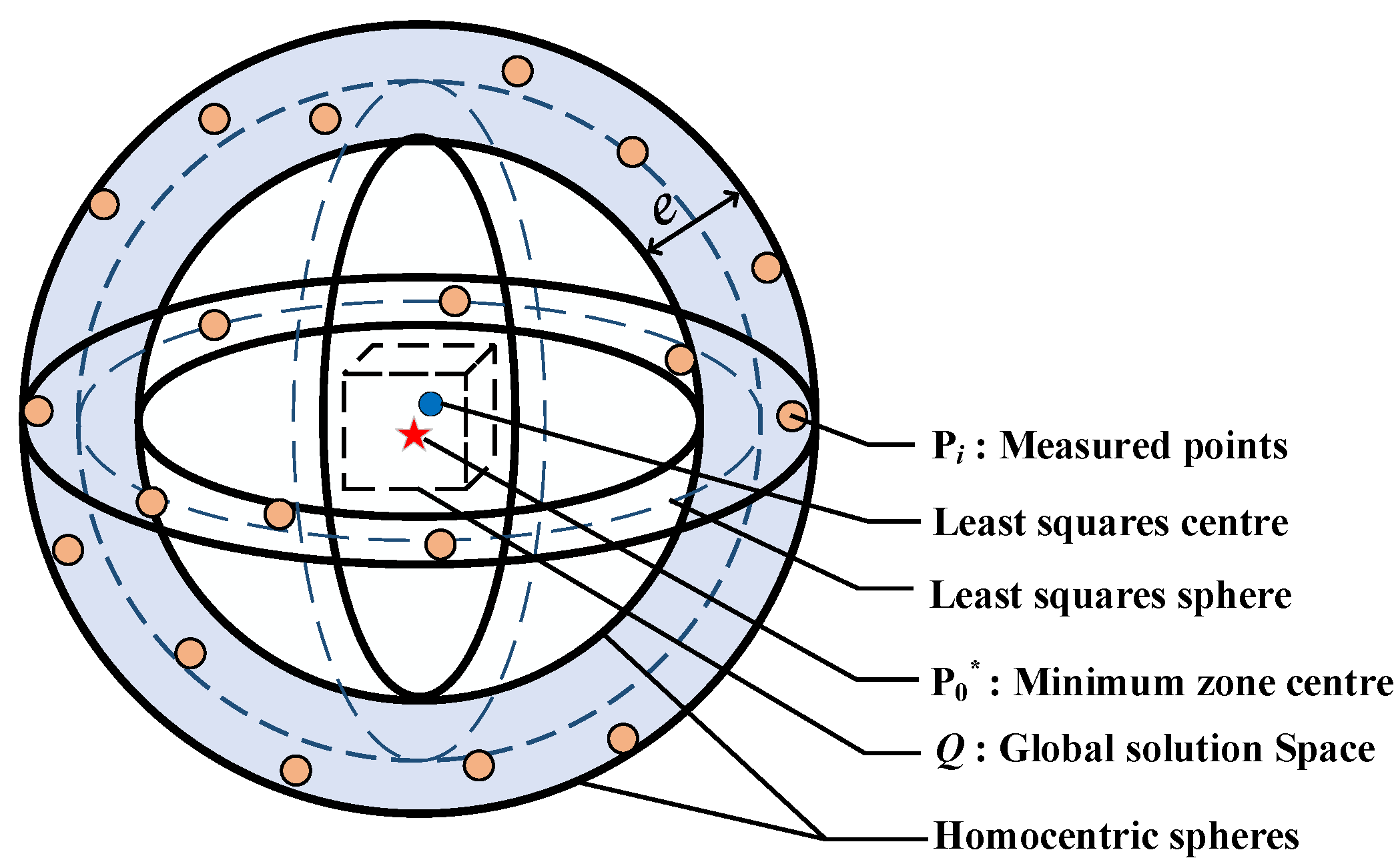
In the equation, e represents the spherical error, where , i = 1, 2, …; n denotes the measurement points in a d-dimensional space; and is the center of the concentric sphere. Q is a cubic region containing the globally optimal solution, which we call the global solution space.
Figure 1 illustrates the spatial geometric structure of spherical error evaluation based on the minimum zone criterion and the various parameters involved. The construction of the global solution space
Q requires the computation of the least squares sphere center and the least squares spherical error based on the least square criterion. Subsequently, a cube with a side length equal to the least squares spherical error is constructed around the least squares sphere center, allowing us to infer that the ideal sphere center must lie within this search region.
2.2. Sphericity Error Spatial Distribution Characteristics
From Equation (1) and
Figure 1, it can be observed that the problem of evaluating the sphericity error based on the minimum zone criterion is non-differentiable and unconstrained. Finding an ideal sphere center
within three-dimensional space, such that the difference in the radii is minimized when the concentric spheres encompass the spherical contour, poses a highly challenging problem. Meanwhile, existing studies suggest that the ideal sphere center
is not unique [
10,
21]. There are several local optimal solutions near the optimal solution of the sphericity error, and the sphericity error decreases rapidly with a large gradient at the location far from the optimal solution [
21].
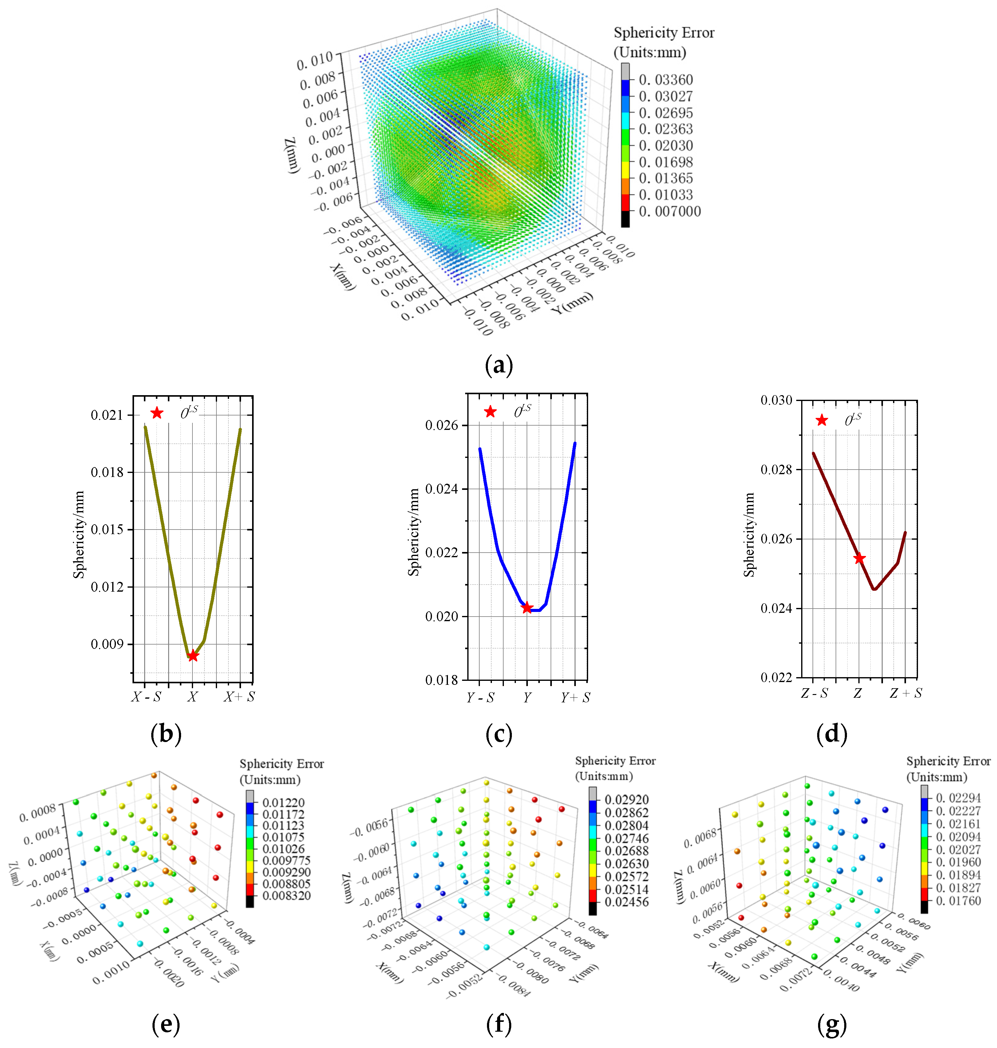
Therefore, we have undertaken a study on the spatial distribution characteristics of spherical error. We conducted an analysis of the data sourced from reference [
15]. Subsequently, we performed 27,000 samplings from the global solution space, calculating the spherical errors for each sampled point.
Figure 2a illustrates the distribution of these sampled points, with the color gradient representing the magnitudes of the associated spherical error values. Following this, within this array of 27,000 points, we scrutinized the variations in spherical error values along the directions parallel to the XYZ axes. This scrutiny was carried out with the center
OLS (X, Y, Z) of the least squares sphere as the central point, independently assessing the variations along each axis.
Meanwhile,
Figure 2b–d show the trend of the sphericity error near the center
OLS (X, Y, Z) of the least squares sphere, where the three lines passing through
OLS and running parallel to the X-axis, Y-axis, and Z-axis, respectively, are constructed. It is clearly discernible from
Figure 2b–d that, at positions considerably distant from the ideal solution, there is a significant gradient in the variation of the spherical error. Conversely, as the position approaches the ideal solution, the evolution of the spherical error gradually becomes more intricate.
Subsequently, we arbitrarily elected several localized solution spaces from the global solution space, analyzing the spherical error variation of the sampling points within these specific solution spaces.
Figure 2e–g illustrate the distribution of sampling points within these localized solution spaces. It can be observed from
Figure 2e–g that within smaller regions, the variation of the spherical error manifests a relatively uncomplicated nature, approximating the characteristics of a unimodal function. If the global solution space is divided into different size subregions, then each subregion can be approximated as a single-peaked function for processing. In local spatial domains, unimodal functions can be effectively solved using computational geometry methods, yielding high-precision results.
The algorithm presented in this paper primarily leverages the characteristics of spherical error gradient variations and the approximate unimodal nature of spherical error changes within local spaces for its design. This is the foundation of the local enhancement principle in this paper.
2.3. Principle of the Proposed Method
As demonstrated in
Section 2, a comprehensive investigation was carried out to analyze the spatial distribution characteristics of the sphericity error. Given the non-uniqueness of the ideal solution
and the potential existence of local optima, the high-precision sphericity error evaluation directly from the global solution space presents a considerable challenge. However, through the adept partitioning of the global solution space into multiple local solutions, it becomes possible to approach the evaluation of the sphericity error as a unimodal function optimization problem within each local space. By employing computational geometry techniques, it is possible to attain high-precision solutions within the confines of these local solution spaces.
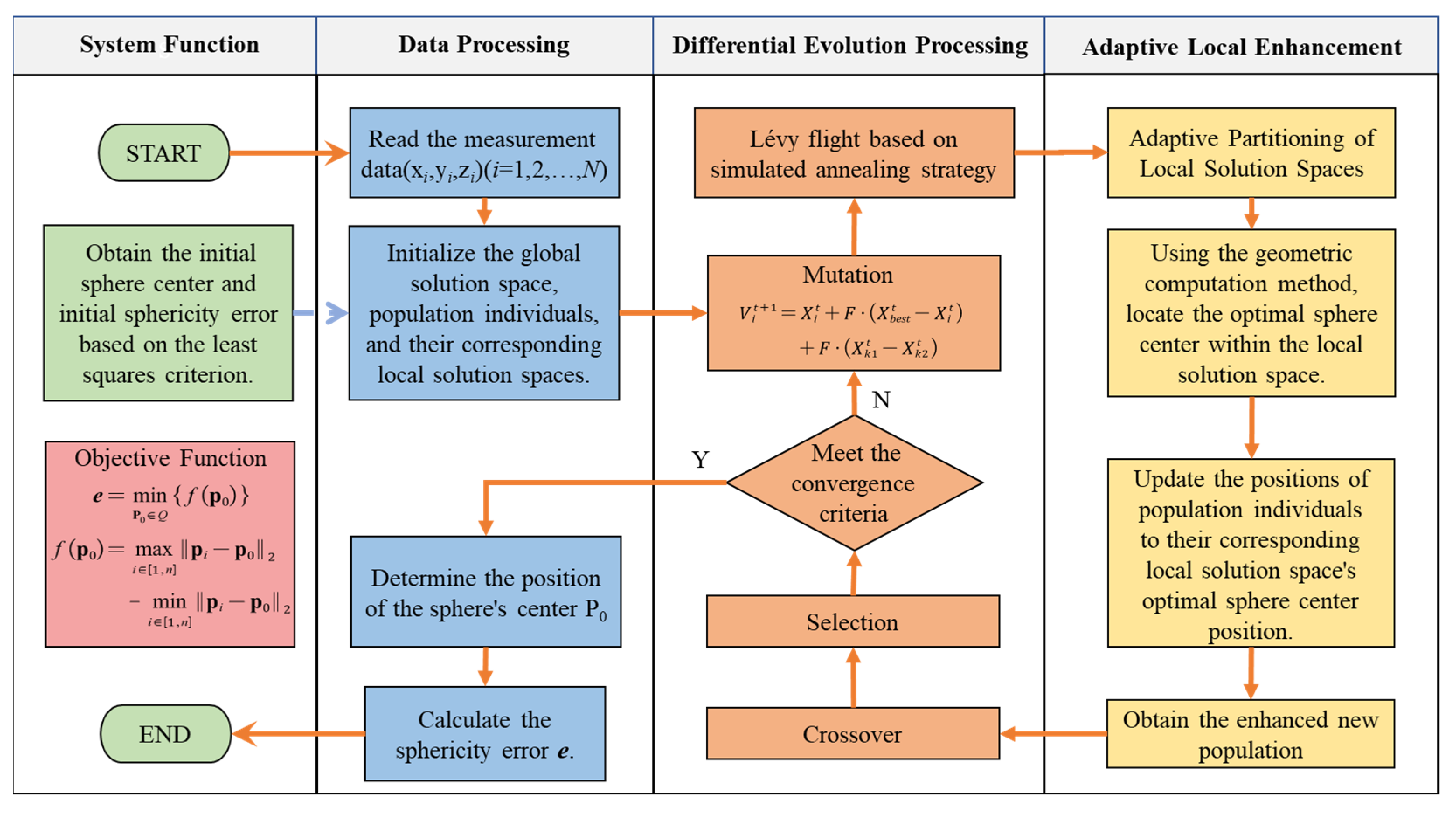
Subsequently, the integration of the computational geometry method employed with the DE algorithm is performed. We establish the positions of local solution spaces by utilizing the individuals that are present in the population of differential evolution. During each iteration, the sizes of the local solution spaces are adaptively adjusted based on the distances between the individuals in the population and the global optimum. Additionally, incorporating Lévy flights and simulated annealing techniques allows for the perturbation of the positions of individuals within the population, thereby augmenting the diversity of local solution spaces. After attaining high-precision solutions within the designated local spaces, the DE algorithm individuals are relocated to their respective optimal positions within these local solution spaces. With each successive iteration of the DE algorithm, the population progressively approaches convergence towards the global optimum. As a result, an optimal solution for minimizing the sphericity error is eventually obtained. The overall algorithmic process is depicted in
Figure 3. We denote the computational geometric method integrated with the DE algorithm as “Adaptive Local Enhancement”. The detailed steps of this approach are outlined in
Section 3.2.
2.4. Adaptive Local Enhancement Method
2.4.1. Adaptive Partitioning of Local Solution Spaces
Considering the gradually complex variations in the sphericity error when the candidate sphere center approaches the ideal sphere center , we devised an adaptive method for partitioning the local solution space. By leveraging the individuals of differential evolution, this method divides the neighborhood of the population into local solution spaces of varying sizes.
During each iteration of the DE algorithm, we calculate the distance denoted as
between an individual’s optimal solution and the population. The determination of the distance is contingent upon the expression
. Subsequently, we determine the size of the individual’s neighborhood space according to
. Here,
K is a scaling factor, and
eps is a constant that prevents
L from becoming zero. The neighborhood search range for each individual, represented as
, falls within the interval of
,
and
.
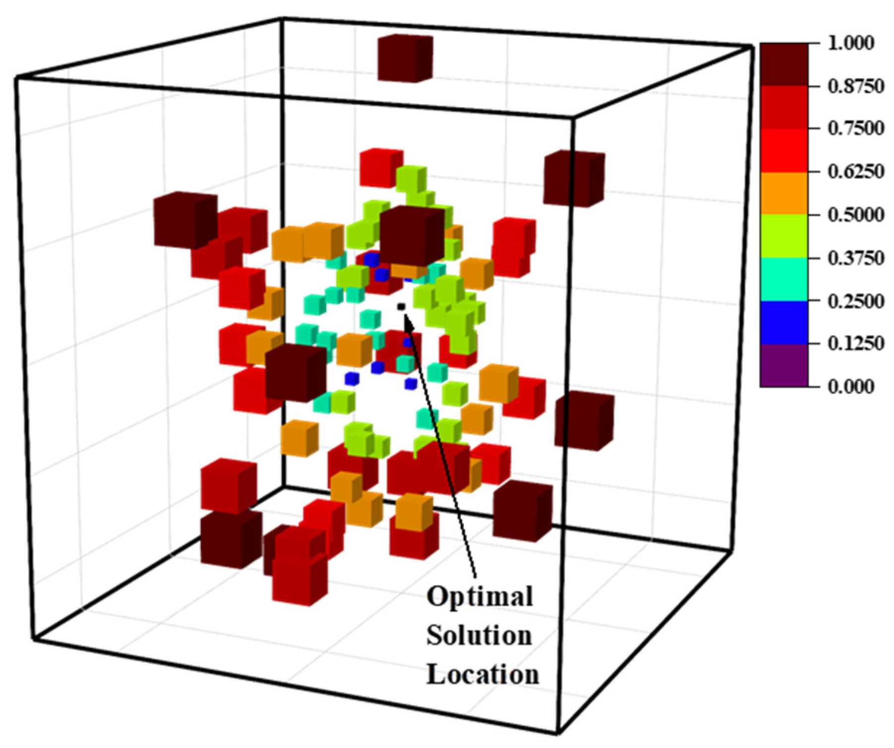
Figure 4 shows the sizes and distributions of these local solution spaces.
2.4.2. Computational Geometric Method for Local Solution Spaces
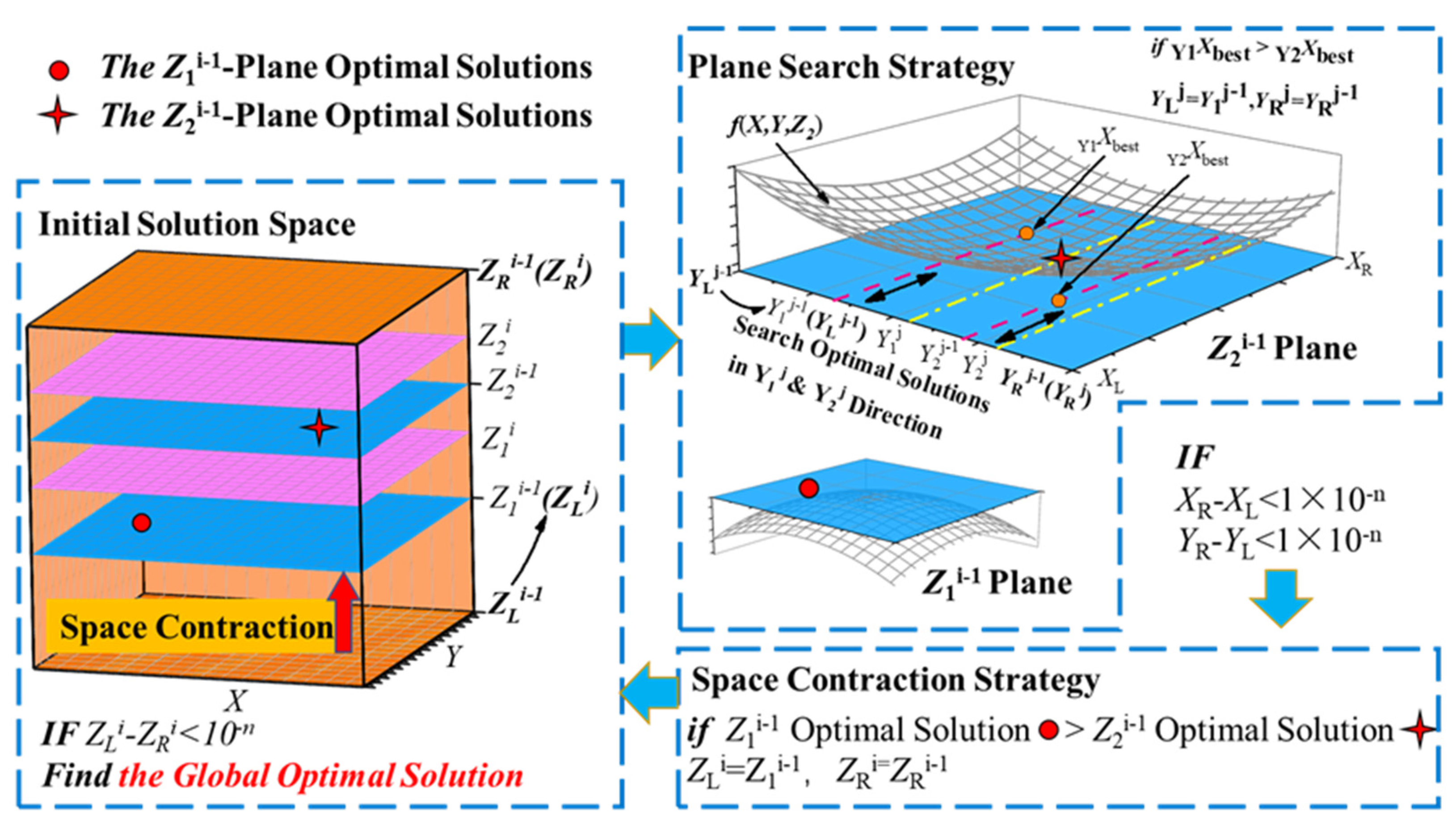
Once the local solution spaces are determined based on the positions of population individuals, a precise solution need to be conducted for each local solution space. Since we regard the problem of solving the spherical deviation error under the constraint of local solution space as a unimodal function problem, we employ the computational geometry approach shown below.
In the three-dimensional space, the local enhancement process of individuals is shown in
Figure 5. According to the predetermined search interval, the initial
Z-directional search interval is determined as
, and then the search is performed on two planes
, where
,
. The initial search interval in the
Y direction is
on two planes
, and a search for the local optimal solution in the one-dimensional direction,
and
, is performed on both planes. Shrinking the search interval according to strategy 1, four positions,
,
,
, and
, of the local optimal solution can be obtained when satisfying the following condition:
XR −
XL < 1 × 10
−n. The local optimal solutions on the
planes are compared, respectively, and the search interval in the
Y-direction on the two planes,
, is shrunken according to strategy 2. After satisfying the condition
YR −
YL < 1 × 10
−n, the optimal solutions
and
on the
planes are obtained. Afterward, the
Z-directional search space is shrunken according to strategy 3. While satisfying
, the local optimal solution is obtained.
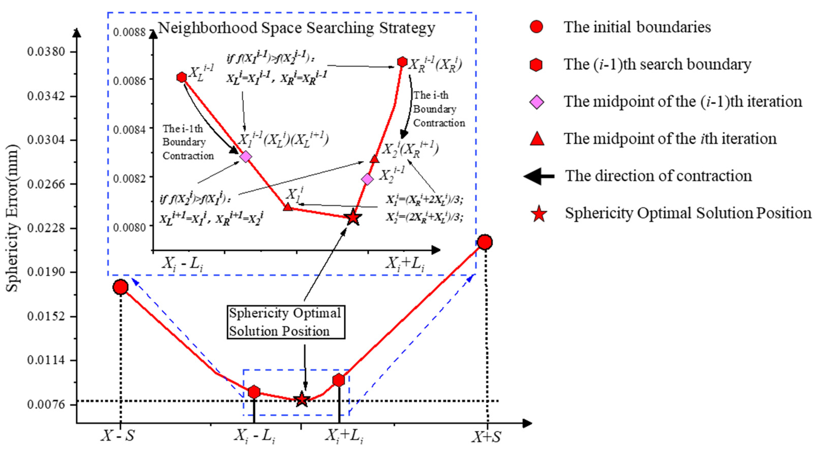
Furthermore, for the one-dimensional search area corresponding to
on the
plane in
Figure 5, the detailed search process is illustrated in
Figure 6. The middle points,
and
, are determined based on the neighborhood searching range of the individuals,
, after which the magnitudes of
and
are compared. If
, then set
; otherwise, set
. Through the strategy above, used to shrink the search interval, the optimal solution is considered as the sphericity error at the
position when
is satisfied.
2.5. Algorithm Flow
2.5.1. Initialization
Firstly, the population and the global temperature of the simulated annealing are initialized, and the initial least square spherical center and least square sphericity error are solved based on the least square solution. The following is the approach for solving the least squares sphericity error S0 and the least squares sphere center OLS based on the least squares criterion. According to the coordinate dataset of the measurement points, , establish the equation set , where , , and . By solving the equation set based on the least square solution, the coordinates of the sphere center OLS and the least square sphericity S0 are obtained. Then, the initial population of the algorithm can be generated in the ranges of ,, and , denoted as X.
2.5.2. Mutation
The mutation strategy is an important part of the DE algorithm. A suitable mutation strategy can promote the convergence of the DE algorithm to the global optimal solution. This algorithm adopts the DE/current-to-best/1/bin strategy, which uses the elite solution to guide the mutation of the existing solutions to approach the optimal one. This mutation strategy is shown in Equation (2).
where
is the
i-th element of the vectors of mutation in the (
t + 1)th generation;
F is the scaling factor and a random number in (0, 0.5);
is the optimal solution in the
t-th generation;
is the
i-th element among the target vectors of the
t-th generation; and
is the random point (
).
2.5.3. Lévy Flight Based on Simulated Annealing Strategy
A Lévy flight perturbed population based on simulated annealing is introduced to enhance the diversity of the local solution space distribution. This strategy enables individuals to explore the global solution space with occasionally long trajectories and short random movements. During the exploration process of the population individuals, their corresponding local solution spaces also move within the solution space. The formula for the Lévy flight in this paper is given by , where ,, and .
The steps of the Lévy flight based on the simulated annealing strategy are as follows:
Step 1: Set an initial temperature T to a sufficiently high value.
Step 2: Consider the original solution of the individuals as S1 and the new solution after Lévy flight perturbation as S2. Calculate the difference df = f (S2) − f (S1) for each individual in the population, where f represents the object function.
Step 3: If df < 0, accept the new solution S2.
Step 4: If df ≥ 0, generate a random number R uniformly distributed in the interval (0, 1) and calculate the acceptance probability exp(−df/T) for S2. If exp(−df/T) > R, accept S2 as the new solution; otherwise, keep the solution unchanged as S1.
Step 5: Reduce the global temperature by setting T = q × T, where q < 1.
As the DE algorithm progresses through iterations, the global temperature gradually decreases, resulting in a reduced probability of accepting inferior solutions. When the temperature reaches a certain threshold, the search process terminates.
2.5.4. Adaptive Local Enhancement
For a comprehensive understanding of the adaptive local enhancement process, please consult
Section 2.4.
Figure 5 illustrates the process of local enhancement.
Once the local solution space’s search range is determined, a local optimal solution would be searched within the local solution spaces using the computational geometric method mentioned earlier. Following a greedy strategy, individuals move to the position of the local solution space’s optimal solution if it is superior to their current position; otherwise, they remain at their initial positions. Then, an enhanced population is generated due to the local enhancement process, denoted as V.
2.5.5. Crossover and Selection
By mixing the new population V and the initial population X with a certain probability, a new population U is generated. Compare each individual in the populations U and X, and retain the ones with smaller sphericity errors for the next iteration.
The loop is ended until the conditions of convergence are satisfied, and the global optimal solution by the minimum zone criterion for evaluating the sphericity error is obtained.
3. Results
3.1. Verification with Datasets in the Literature
Due to the limited availability of publicly accessible datasets in the field of sphericity error research, current research papers often refer to the same set of publicly available spherical datasets for comparative analyses. Notably, the four datasets [
15,
16,
31,
33] used in the experiments of this section have been widely cited in numerous high-quality publications in the field of sphericity error research. As a result, these datasets hold considerable authority. By conducting experiments using these four datasets, we can effectively compare our approach with the leading algorithms in the field of sphericity error evaluation under identical experimental conditions. This reasoning highlights one of the main reasons for selecting these four datasets for experimentation in our study.
The experiments were conducted under identical conditions. The number of populations (N) was set to 30, the local enhancement parameter (n) was set to 12, the initial temperature (T) was set to 100, the annealing rate (q) was set to 0.9, and the temperature threshold was set to 0.001. Using the aforementioned settings, each dataset was independently calculated ten times. The mean and standard deviation of the results were calculated and compared with the results obtained using state-of-the-art algorithms.
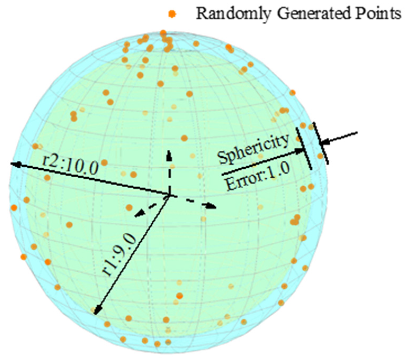
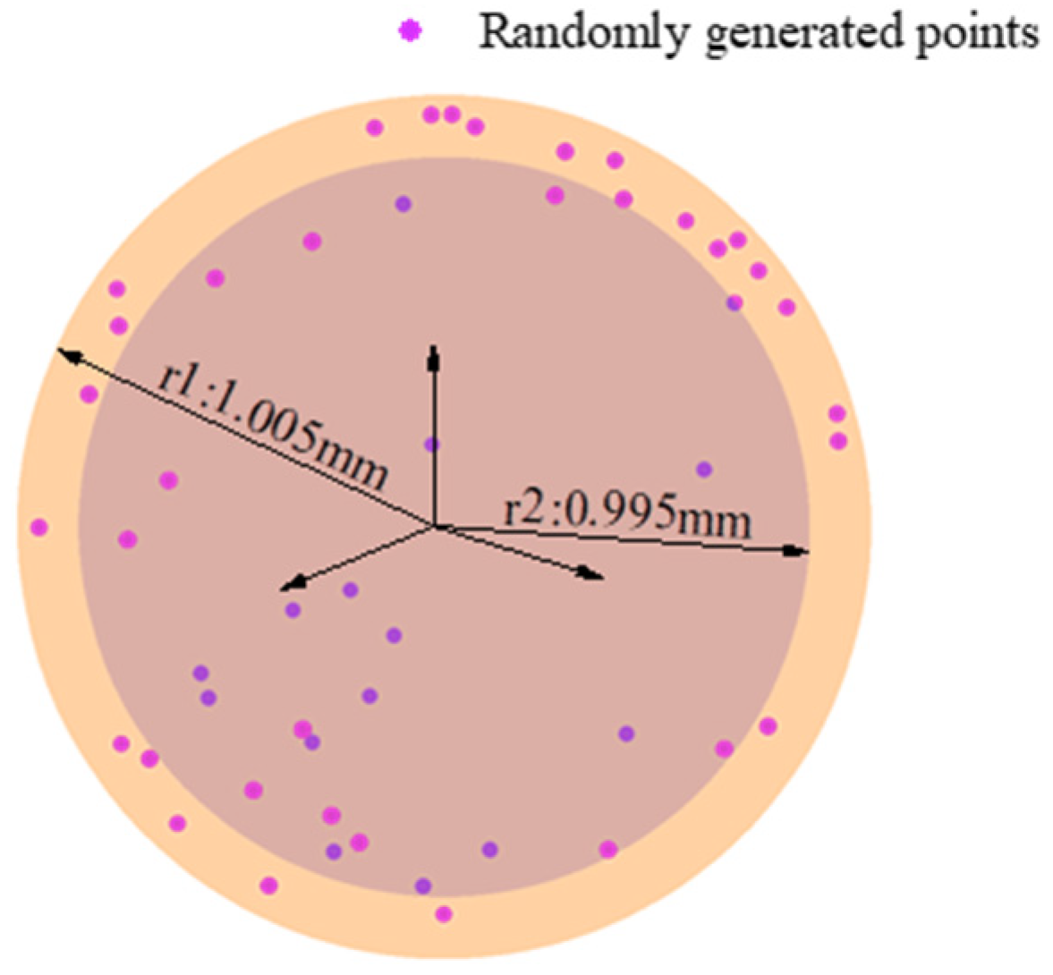
Dataset 1, obtained from reference [
34], comprises 100 randomly generated coordinate points within two concentric spheres with radii of 10.0 and 9.0. The data distribution is illustrated in
Figure 7, where the sphericity error is determined as 1.0 based on five data points from the inner and outer spheres. The sphericity error of dataset 1 has been validated in several studies [
21,
34], and the algorithm’s accuracy in this paper was initially assessed using dataset 1.
Ten sets of replication experiments were performed for dataset 1. The mean experimental result is 1.00000000000003 mm, with a standard deviation of 2.0 × 10
−14 mm.
Figure 8 displays one convergence curve from the ten experiments.
Table 1 presents a comparison with the results reported in the literature.
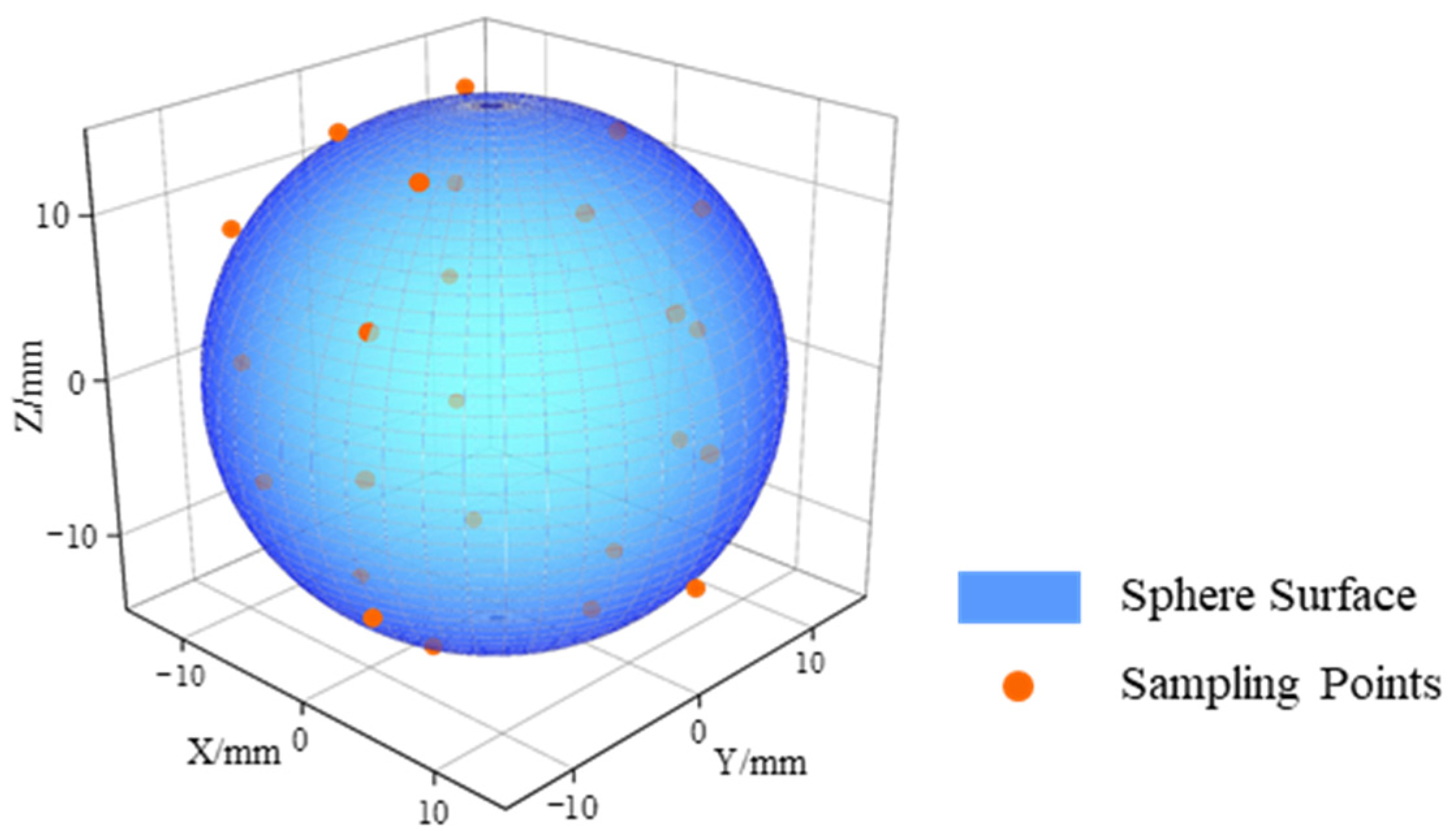
Dataset 2, consisting of 384 coordinate points, is provided in reference [
16]. The 384 coordinate points were obtained through real spherical sampling using the birdcage method and were evenly distributed along 12 lines on the sphere.
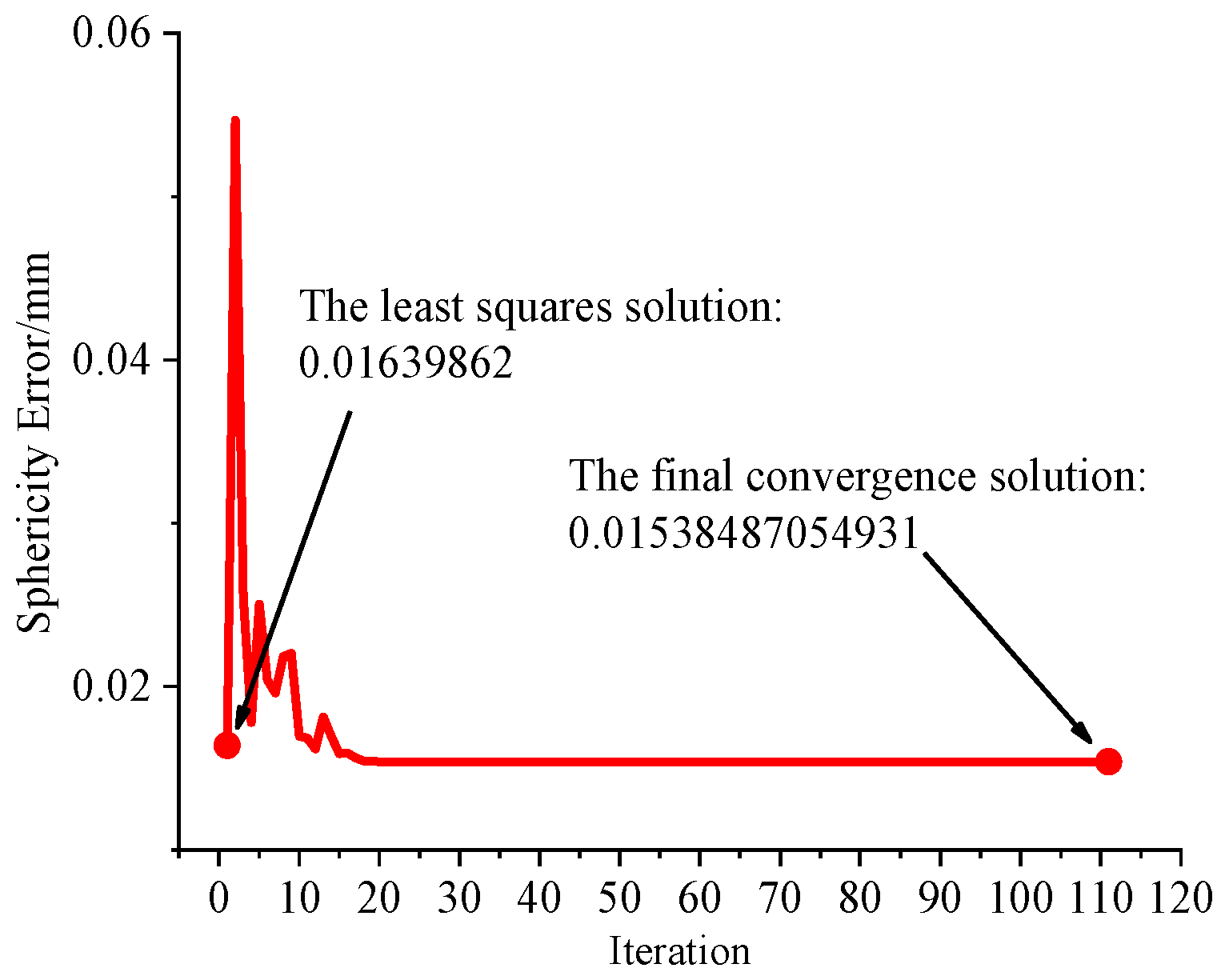
Figure 9 illustrates the distribution of dataset 2. The reference provides the optimal solution as 0.015385 mm. Ten sets of replication experiments were conducted for dataset 2.
Table 2 presents the results of the ten experiments, with a mean experimental result of 0.01538487054930 mm and a standard deviation of 3.0 × 10
−14 mm.
Figure 10 displays one convergence curve from the ten experiments. The least square solution obtained by our algorithm is 0.01639862 mm, and the final convergence solution is 0.01538487054931 mm.
Table 3 presents a comparison with the results reported in the literature.
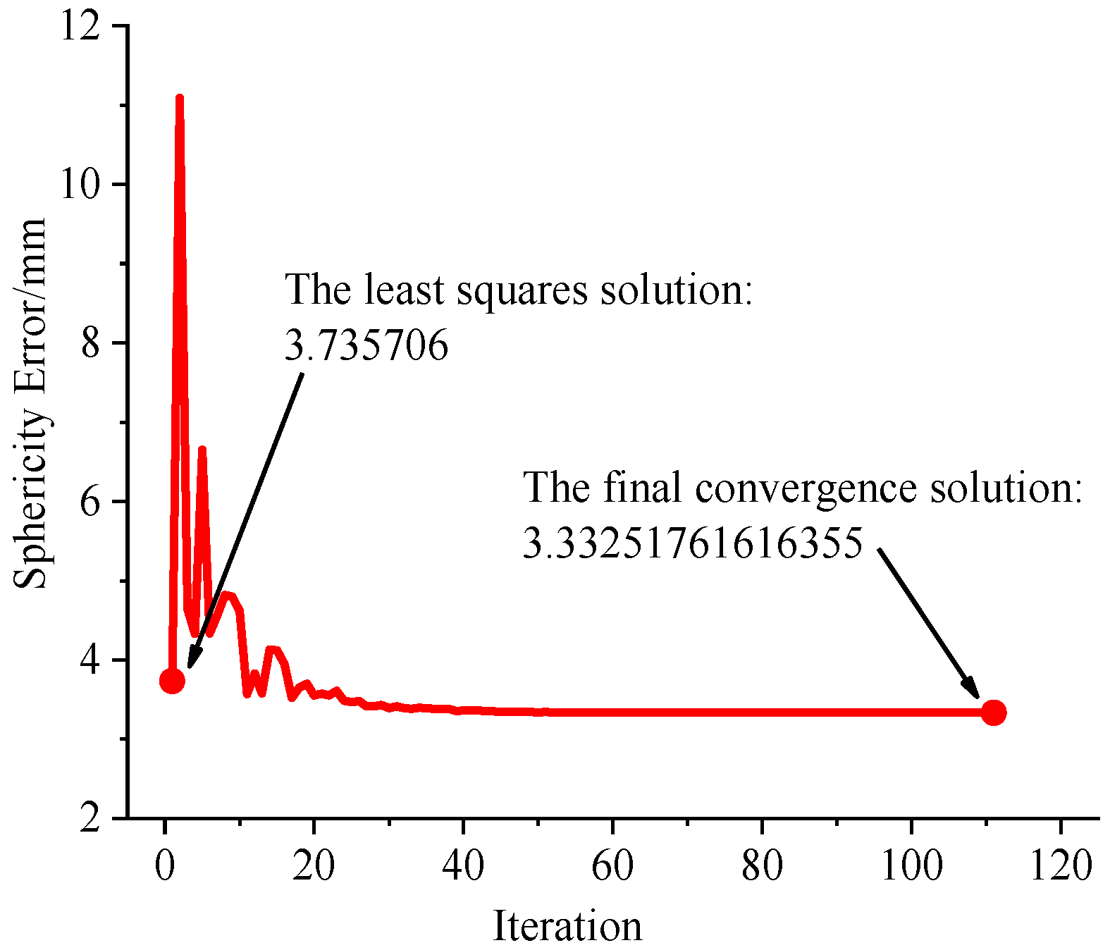
Dataset 3, consisting of 25 coordinate points, is provided in reference [
36].
Figure 11 illustrates the distribution of dataset 3, with the coordinate points uniformly distributed on the sphere. Ten sets of replication experiments were conducted for dataset 3.
Table 4 presents the results of the ten experiments, with a mean experimental result of 3.33251761616355 mm and a standard deviation of 0.8 × 10
−14 mm.
Figure 12 displays a convergence curve from one of the ten experiments. The least square solution obtained by our algorithm is 3.735706 mm, and the final converged solution is 3.33251761616355 mm.
Table 5 presents a comparison with the results reported in the literature.
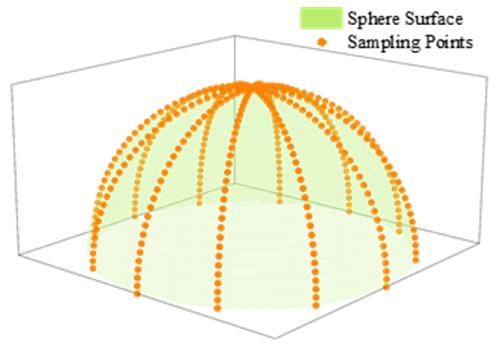
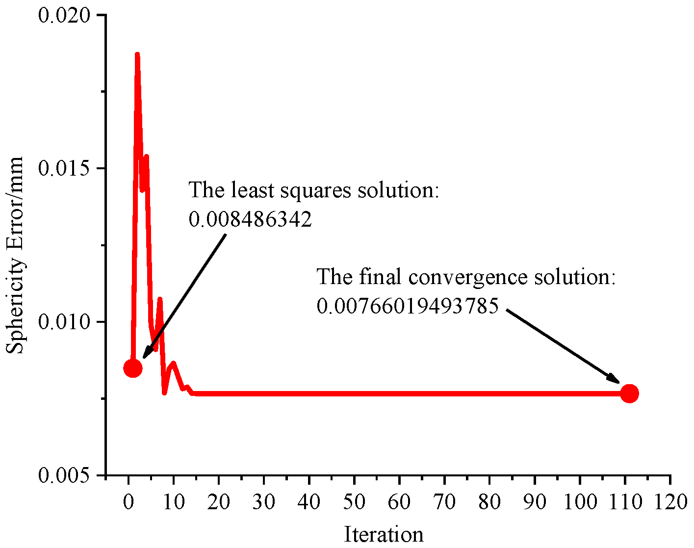
Dataset 4, consisting of 50 coordinate points, is provided in reference [
15].
Figure 13 illustrates the distribution of dataset 4, with the coordinate points randomly distributed on the sphere. Ten sets of replication experiments were conducted for dataset 4.
Table 6 presents the results of the ten experiments, with a mean experimental result of 0.00766019493788 mm and a standard deviation of 0.2 × 10
−14 mm.
Figure 14 displays a convergence curve from one of the ten experiments. The least square solution obtained by our algorithm is 0.008486342 mm, and the final converged solution is 0.00766019493785 mm.
Table 7 presents a comparison with the results reported in the literature.
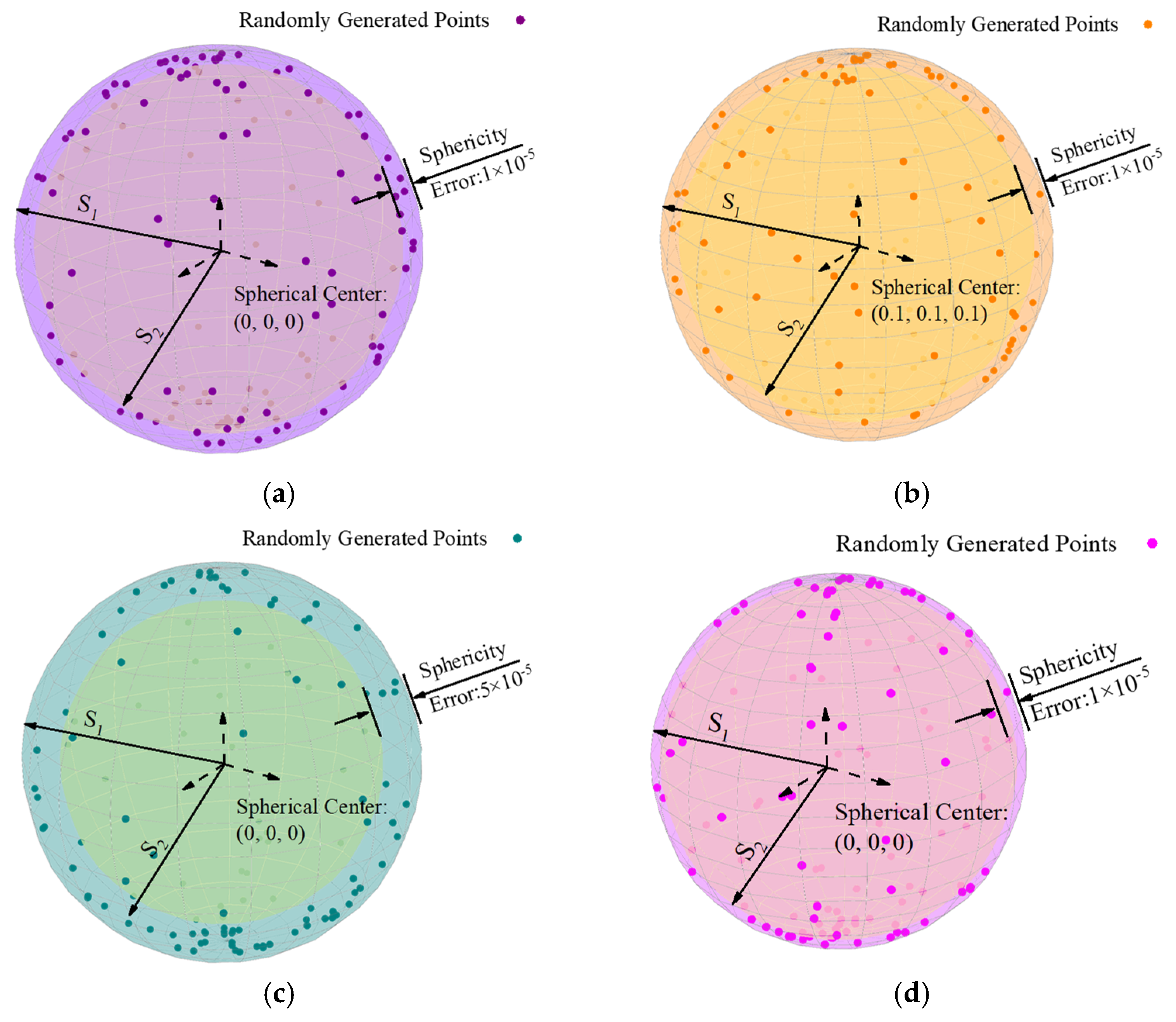
3.2. Simulated Experiments
To further assess the algorithm’s accuracy, we employed the methodology described in reference [
34] to generate simulated data, creating four distinct datasets. Initially, two concentric spherical surfaces,
and
, were established with radii
and
, where
, and
e represents the simulated spherical error.
The points on these concentric spheres were identified as control points, with ten control points generated on each inner and outer sphere. Utilizing Formula (3), by randomly generating values for
and
, we generated 100 random sampling points within the concentric sphere, culminating in a dataset comprising 120 simulated sampling points. The 20 control points on both the inner and outer spheres effectively constrained the spherical error of the simulated dataset to the difference in the radii between the inner and outer spheres.
Table 8 provides comprehensive information of the spherical error, center coordinate, radii, and the number of simulated sampling points for each of the four datasets. Additionally,
Figure 15 visually portrays the data distribution of these four simulated datasets.
We conducted ten experiments for each dataset, showcasing the optimal estimates and standard deviations in
Table 9. Furthermore, detailed simulated data are provided in
Appendix B,
Table A2,
Table A3,
Table A4 and
Table A5.
Table 9 shows that the algorithm’s solutions for spherical error exhibit a deviation within the magnitude of 10
−14 mm from the ideal spherical error. Moreover, the standard deviation of the results from ten experiments also lies within the magnitude of 10
−14 mm. The results attest to the algorithm’s successful identification of the ideal sphere center and spherical error.
3.3. Ablation Experiment
From the perspective of the algorithmic framework, this algorithm is based on the differential evolution algorithm, thus sharing evident similarities with traditional single-objective search algorithms. The algorithm is specifically designed to address the distribution characteristics of the sphericity error. It proposes that the resolution of the sphericity error can be treated as a unimodal function in the local solution space. Subsequently, the local enhancement method for solving this unimodal function is synergistically integrated with the differential evolution algorithm, demonstrating higher precision and robustness.
To delve into the pivotal aspects of the algorithm in this paper, we conducted ablation experiments, employing the same parameter configuration outlined in
Section 3.1. We designated the algorithm with the removal of local enhancement steps as algorithm A and designated the algorithm retaining these steps as algorithm B. Subsequently, ten experiments were performed for each algorithm, with the standard deviation of the results computed. The experimental findings are documented in
Table 10, from which it is evident that removing local enhancement methods significantly diminishes the algorithm’s robustness, reducing the standard deviation from a magnitude of 10
−14 mm to a magnitude of 10
−2~10
−7 mm. This experiment’s results substantiate the favorable outcome achieved by amalgamating the proposed local enhancement method and differential evolution algorithm in this paper.
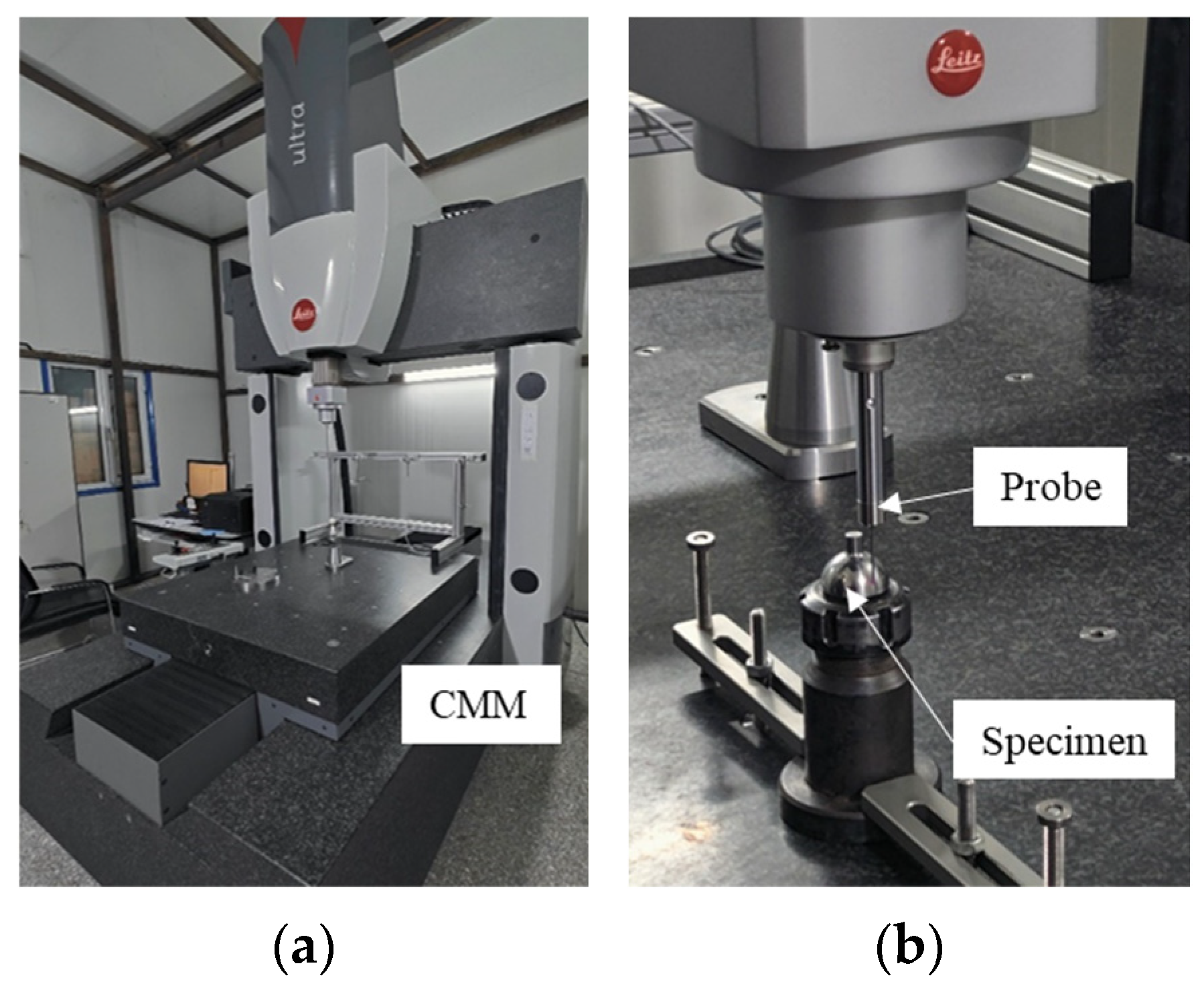
3.4. Experiments with Datasets Obtained from CMM
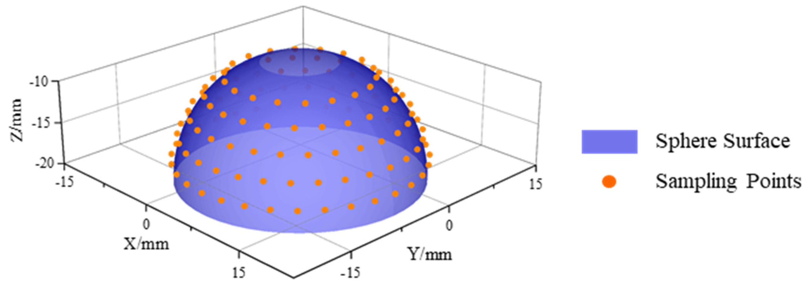
To assess the proposed method’s practicality, we measured a metal hemispherical shell resonator, as depicted in
Figure 16b. The measurements were carried out in a controlled environment, as shown in
Figure 16a, using a Hexagon CMM.
For the measurement of the specimen, we selected five cross-sections on the surface. As detailed in
Table A1, one hundred and thirty measurement points were taken. The iterative process convergence, reconstruction model of the dataset, and evaluation results are presented in
Figure 17 and
Figure 18.
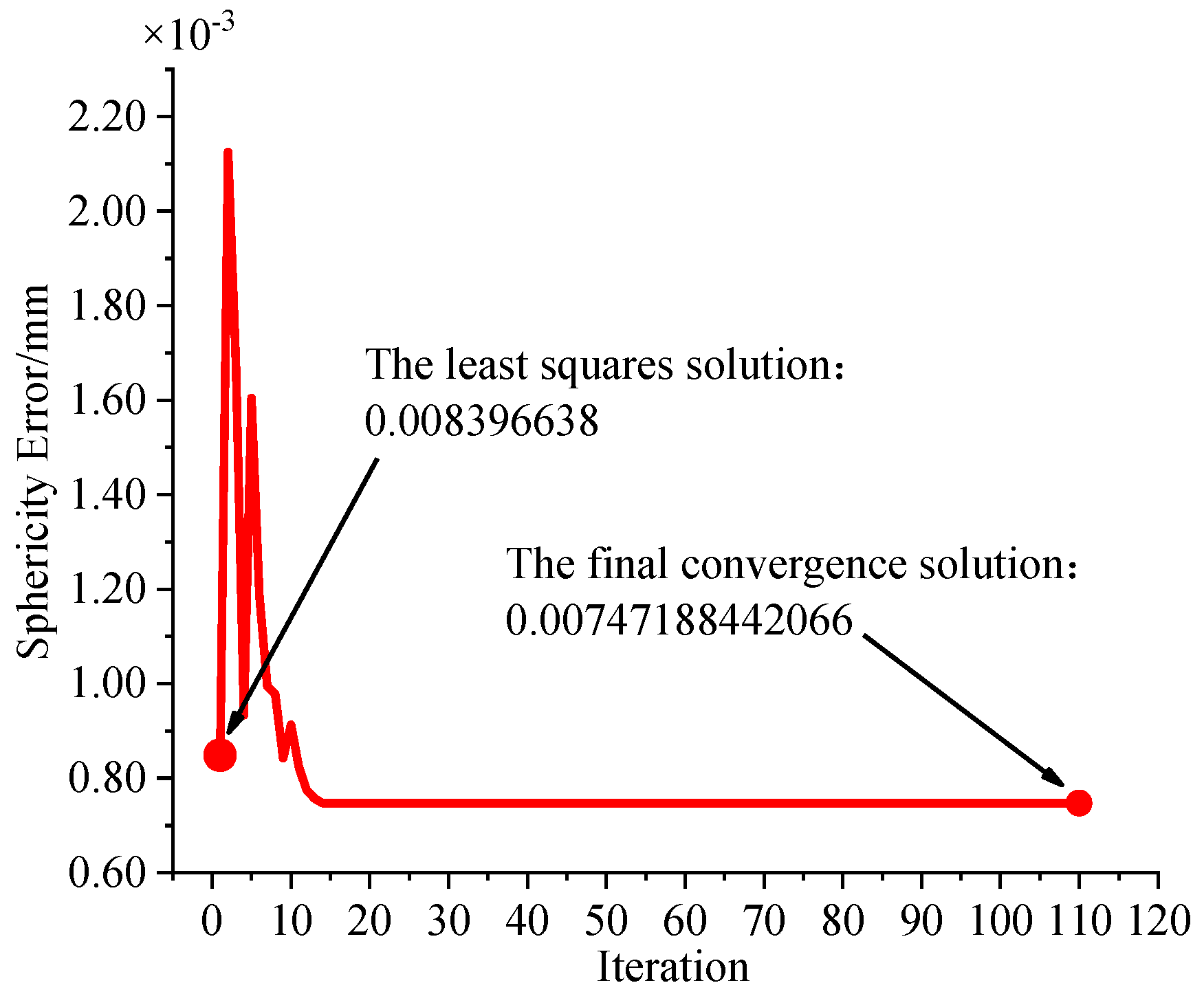
Ten replication experiments were conducted for the measurement data. The sphericity error obtained by the CMM is 0.008396638 mm. The results of these ten experiments are presented in
Table 11, indicating a mean result of 0.00747188442066 mm, with a standard deviation of 2.3 × 10
−14 mm. The spherical center obtained by our algorithm is (0.00218039158405 mm, −0.00226432610011 mm, −23.9943439405 mm). Our algorithm demonstrated an 11% improvement in accuracy compared to the CMM result.
4. Discussion
Evaluating the sphericity error based on the minimum zone criterion is an indispensable and challenging task in metrology. Thus, this study aims to achieve a high-precision evaluation of spherical contour sampling data. Consequently, we conducted an in-depth investigation into the spatial distribution characteristics of the sphericity error. We propose treating the local space of the sphericity error as a unimodal function and utilizing computational geometry methods to obtain high-precision solutions for the local space. Subsequently, combined with the advantages of heuristic algorithms in searching the global space, we successfully achieved exact solutions for sphericity errors.
To validate the efficacy of the proposed approach, we conducted experiments using datasets that are widely cited in the realm of spherical error research, which are featured in four high-level scholarly papers. The experimental results demonstrate a significant improvement in precision, surpassing the existing achievements in the field of spherical error research by several orders of magnitude. Meanwhile, the uncertainty of the algorithm’s solution reaches 10−14 orders of magnitude, which far exceeds that of the traditional heuristic algorithm. Furthermore, when processing the distribution of data with specific sphericity or dealing with a large number of data points, the global optimal solution can be searched out accurately using the proposed algorithm, which shows stronger robustness.
Subsequently, we conducted ablation experiments on the four datasets, as mentioned earlier. The experimental results show that, after removing the local enhancement method, the algorithm’s standard deviation decreases from the order of 10−14 mm to the order of 10−2~10−7 mm. The ablation experiments demonstrate the effectiveness of the proposed local enhancement method in this paper.
Finally, we apply the algorithm to evaluate the sphericity errors of the hemispherical shell resonator and obtain its sphericity error of 0.00747188442066 mm with a standard deviation of 2.3 × 10⁻¹⁴ mm for ten experiments. Compared to the results obtained from the CMM, this algorithm can improve the accuracy of sphericity error evaluation by approximately 10%.
In this study, each member of the population in the DE algorithm is considered the center point for partitioning local solution spaces. During each iteration of the algorithm, computational geometric techniques are employed to solve for these individual local solution spaces. This approach has yielded outstanding precision in evaluating sphericity errors. However, it has also resulted in an algorithmic time complexity of O(n4), leading to elevated time costs for each evaluation. Furthermore, we conducted assessments of the average time required for each evaluation. Under the specified parameter settings, completing a single evaluation takes approximately 300 s. Compared to the time costs of 0.1 to 1 s in existing studies, the average time cost of our algorithm has increased several-fold. It must be acknowledged that this algorithm is not suitable for components with spherical geometry that require large-scale production and have relatively low precision requirements, such as ball bearings. In these contexts, the speed of the sphericity error assessment takes precedence over precision. However, for crucial spherical components in the entire realm of research that necessitate only one or two ultra-high precision devices, such as the ball bearings in astronomical telescopes and the electrostatic rotor in Gravity Probe B, the precision and reliability of the sphericity error assessment outweighs speed. Nevertheless, pursuing high speed and precision remains a common goal across all research domains. Therefore, reducing time costs while maintaining the existing precision level is a critical direction for future research improvements.
In summary, this study proposes an algorithm that is aimed at the high-precision evaluation of sphericity errors and that is capable of performing a highly accurate evaluation of sphericity errors. However, to achieve this high precision in sphericity error evaluation, the algorithm has made certain sacrifices in terms of the time cost. This method provides practical tools and techniques for applying ultra-precision spheres in precision engineering. It introduces new perspectives for sphericity error evaluation based on the minimum zone criterion.
Author Contributions
Conceptualization, D.Z. and J.C.; methodology, D.Z.; software, D.Z.; validation, J.C.; formal analysis, D.Z.; investigation, D.Z. and J.C.; resources, J.C., Z.W. and Y.S.; data curation, D.Z.; writing—original draft preparation, D.Z.; writing—review and editing, D.Z.; visualization, D.Z., Z.W. and Y.S.; supervision, J.C.; project administration, J.C.; funding acquisition, J.C. All authors have read and agreed to the published version of the manuscript.
Funding
This work was supported by the National Natural Science Foundation of China of No. 52075133.
Institutional Review Board Statement
Not applicable.
Informed Consent Statement
Not applicable.
Data Availability Statement
All data that support the findings of this study are included within this article.
Conflicts of Interest
The authors declare that they have no known competing financial interests or personal relationships that could have appeared to influence the work reported in this paper.
Appendix A
Table A1.
CMM raw coordinate indication point dataset from a hemispherical shell resonator measurement (units: mm).
Table A1.
CMM raw coordinate indication point dataset from a hemispherical shell resonator measurement (units: mm).
| No. | X | Y | Z | No. | X | Y | Z |
|---|
| 1 | 8.296414 | −3.02143 | −11.3267 | 66 | 11.61279 | 5.831947 | −15.6435 |
| 2 | 6.763515 | −5.67803 | −11.3267 | 67 | 12.64508 | 2.993801 | −15.6456 |
| 3 | 4.413842 | −7.64931 | −11.3266 | 68 | 12.99436 | 0.00061 | −15.6446 |
| 4 | 1.53153 | −8.6978 | −11.3264 | 69 | 14.36486 | 0.00079 | −18.3304 |
| 5 | −1.53198 | −8.69712 | −11.3262 | 70 | 14.05059 | 2.984275 | −18.3304 |
| 6 | −4.41293 | −7.6497 | −11.3271 | 71 | 13.12312 | 5.840188 | −18.3305 |
| 7 | −6.76176 | −5.67733 | −11.3264 | 72 | 11.62104 | 8.44174 | −18.3301 |
| 8 | −8.2954 | −3.02146 | −11.3276 | 73 | 9.610385 | 10.67402 | −18.33 |
| 9 | −8.82762 | 0.00175 | −11.3272 | 74 | 7.180646 | 12.43983 | −18.33 |
| 10 | −8.29549 | 3.019205 | −11.3266 | 75 | 4.436134 | 13.66083 | −18.3294 |
| 11 | −6.76226 | 5.675262 | −11.3273 | 76 | 1.499609 | 14.28478 | −18.3294 |
| 12 | −4.41211 | 7.645938 | −11.3277 | 77 | −1.50034 | 14.28458 | −18.3299 |
| 13 | −1.53142 | 8.694617 | −11.3278 | 78 | −4.43637 | 13.66036 | −18.3297 |
| 14 | 1.53211 | 8.694537 | −11.3271 | 79 | −7.17943 | 12.43851 | −18.33 |
| 15 | 4.413092 | 7.645988 | −11.3269 | 80 | −9.60919 | 10.673 | −18.3294 |
| 16 | 6.763165 | 5.674052 | −11.3267 | 81 | −11.6198 | 8.44048 | −18.3295 |
| 17 | 8.296184 | 3.017535 | −11.3274 | 82 | −13.1219 | 5.839438 | −18.3305 |
| 18 | 8.828784 | 0.00144 | −11.3275 | 83 | −14.0492 | 2.983165 | −18.3305 |
| 19 | 11.12424 | 0.0013 | −13.2813 | 84 | −14.3622 | 0.00134 | −18.3307 |
| 20 | 10.71211 | 2.999729 | −13.2816 | 85 | −14.0472 | −2.98888 | −18.3309 |
| 21 | 9.505538 | 5.779181 | −13.2803 | 86 | −13.1193 | −5.84373 | −18.331 |
| 22 | 7.592488 | 8.12935 | −13.2799 | 87 | −11.6175 | −8.44454 | −18.3309 |
| 23 | 5.115596 | 9.876324 | −13.2799 | 88 | −9.60736 | −10.6763 | −18.3306 |
| 24 | 2.260611 | 10.89058 | −13.2814 | 89 | −7.17731 | −12.4413 | −18.3302 |
| 25 | −0.75887 | 11.09661 | −13.2814 | 90 | −4.43455 | −13.6626 | −18.3298 |
| 26 | −3.72318 | 10.48024 | −13.2821 | 91 | −1.49886 | −14.287 | −18.33 |
| 27 | −6.41267 | 9.08655 | −13.2818 | 92 | 1.500999 | −14.2875 | −18.3296 |
| 28 | −8.62704 | 7.018315 | −13.2813 | 93 | 4.437544 | −13.6644 | −18.3289 |
| 29 | −10.2019 | 4.429719 | −13.2817 | 94 | 7.181086 | −12.4437 | −18.3295 |
| 30 | −11.0187 | 1.511798 | −13.2827 | 95 | 9.611795 | −10.6784 | −18.3291 |
| 31 | −11.0178 | −1.51657 | −13.2831 | 96 | 11.62196 | −8.44553 | −18.3291 |
| 32 | −10.2016 | −4.43394 | −13.2835 | 97 | 13.12441 | −5.84411 | −18.33 |
| 33 | −8.62646 | −7.02263 | −13.2815 | 98 | 14.05164 | −2.98806 | −18.33 |
| 34 | −6.41128 | −9.08998 | −13.2814 | 99 | 14.90208 | −2.96403 | −21.2295 |
| 35 | −3.72154 | −10.4842 | −13.2812 | 100 | 14.03837 | −5.81562 | −21.2292 |
| 36 | −0.75777 | −11.0995 | −13.2808 | 101 | 12.63434 | −8.44279 | −21.2289 |
| 37 | 2.261661 | −10.8914 | −13.2782 | 102 | 10.74393 | −10.7462 | −21.2288 |
| 38 | 5.116226 | −9.87919 | −13.2798 | 103 | 8.43965 | −12.6363 | −21.2285 |
| 39 | 7.592868 | −8.13236 | −13.2797 | 104 | 5.8119 | −14.04 | −21.2286 |
| 40 | 9.505198 | −5.78223 | −13.2807 | 105 | 2.961514 | −14.9037 | −21.2287 |
| 41 | 10.71221 | −3.00317 | −13.2805 | 106 | −0.00016 | −15.1941 | −21.2291 |
| 42 | 12.64529 | −2.99836 | −15.6442 | 107 | −2.96109 | −14.9016 | −21.229 |
| 43 | 11.61302 | −5.83438 | −15.6435 | 108 | −5.81005 | −14.0377 | −21.2287 |
| 44 | 9.954915 | −8.35568 | −15.6437 | 109 | −8.43761 | −12.633 | −21.2283 |
| 45 | 7.759662 | −10.4272 | −15.6439 | 110 | −10.7396 | −10.7434 | −21.229 |
| 46 | 5.14489 | −11.9356 | −15.6438 | 111 | −12.6302 | −8.44041 | −21.2291 |
| 47 | 2.254347 | −12.8003 | −15.6441 | 112 | −14.0335 | −5.81371 | −21.2291 |
| 48 | −0.75498 | −12.9743 | −15.6445 | 113 | −14.8978 | −2.96381 | −21.2286 |
| 49 | −3.72379 | −12.4499 | −15.6451 | 114 | −15.1907 | −0.00053 | −21.2288 |
| 50 | −6.49358 | −11.2552 | −15.6455 | 115 | −14.9 | 2.961734 | −21.2291 |
| 51 | −8.91403 | −9.45329 | −15.6456 | 116 | −14.036 | 5.81165 | −21.2281 |
| 52 | −10.8542 | −7.14139 | −15.6459 | 117 | −12.6318 | 8.43835 | −21.2283 |
| 53 | −12.2073 | −4.44475 | −15.6464 | 118 | −10.741 | 10.74128 | −21.2287 |
| 54 | −12.9032 | −1.50946 | −15.647 | 119 | −8.43702 | 12.63058 | −21.2273 |
| 55 | −12.9038 | 1.506108 | −15.6464 | 120 | −5.81015 | 14.0345 | −21.2297 |
| 56 | −12.2085 | 4.442633 | −15.6461 | 121 | −2.9605 | 14.89967 | −21.229 |
| 57 | −10.8544 | 7.138399 | −15.6462 | 122 | 0.00035 | 15.19031 | −21.2285 |
| 58 | −8.91463 | 9.450499 | −15.6466 | 123 | 2.962754 | 14.8987 | −21.2293 |
| 59 | −6.49321 | 11.25221 | −15.6457 | 124 | 5.81229 | 14.03412 | −21.2292 |
| 60 | −3.72336 | 12.44723 | −15.6456 | 125 | 8.43856 | 12.63031 | −21.2276 |
| 61 | −0.75426 | 12.97149 | −15.6459 | 126 | 10.74231 | 10.73945 | −21.2293 |
| 62 | 2.254877 | 12.79544 | −15.6441 | 127 | 12.63195 | 8.4362 | −21.2295 |
| 63 | 5.14524 | 11.93096 | −15.6447 | 128 | 14.03555 | 5.80935 | −21.2291 |
| 64 | 7.760032 | 10.42313 | −15.6465 | 129 | 14.89984 | 2.960004 | −21.229 |
| 65 | 9.956695 | 8.350528 | −15.6449 | 130 | 15.19234 | 0.00022 | −21.229 |
Appendix B
Table A2.
Simulation dataset A’s coordinate data (units: mm).
Table A2.
Simulation dataset A’s coordinate data (units: mm).
| No. | X | Y | Z | No. | X | Y | Z |
|---|
| 1 | 2.70716589312049 | 5.50739356847015 | 7.89557274104917 | 61 | −2.89280574054528 | −3.65641016545042 | 8.84661176098279 |
| 2 | −1.15214718780568 | −9.20081371548616 | 3.74402430584425 | 62 | −1.51828118667085 | −9.13434218820972 | −3.77606589087291 |
| 3 | −1.01772769992569 | −1.84485104912249 | 9.77552546524520 | 63 | 2.24430605422733 | −4.05526495095270 | −8.86103883157432 |
| 4 | 1.09745748886757 | 8.99030141206831 | 4.23912436513771 | 64 | 1.00655478403967 | 2.74990194311456 | 9.56164599503323 |
| 5 | −1.28865793782677 | −2.14712961492406 | 9.68138493151514 | 65 | −5.91008390550214 | 6.65426786156021 | 4.55980563803232 |
| 6 | 2.23712088095506 | −5.64280260263515 | 7.94695444739222 | 66 | 1.05649986536444 | 3.12247361232877 | −9.44108128748343 |
| 7 | 0.96389378689230 | 9.38875252004527 | −3.30491072270252 | 67 | 7.85501071612662 | 2.19242740865312 | −5.78724691162584 |
| 8 | 0.09516036830667 | 0.57085048124596 | −9.98324191519372 | 68 | −7.39966754477964 | −4.84965141456539 | 4.66109444057282 |
| 9 | 3.85822591335003 | 4.61648956587795 | −7.98762771847785 | 69 | 1.09631832016297 | −7.49379191536427 | −6.53003590114144 |
| 10 | −1.06721159538523 | 1.93885104125363 | −9.75203135750703 | 70 | 3.53745810772145 | −1.78161148450475 | −9.18217909565151 |
| 11 | 6.26235696234287 | −7.59196187568609 | 1.77341482860745 | 71 | 6.76213768840946 | −0.59511144741485 | 7.34298594770830 |
| 12 | −2.62499745458919 | 9.43001171406783 | 2.04554819936948 | 72 | −7.89611121553721 | −3.79056887081821 | −4.82525144178618 |
| 13 | 0.29152155597613 | 8.30981199131132 | 5.55536918545053 | 73 | −3.45995327527011 | −1.48232328353041 | −9.26452594664461 |
| 14 | 0.20630522606167 | 2.26036506127748 | 9.73900572541429 | 74 | −0.44629221645521 | −7.21658669463085 | −6.90809564438316 |
| 15 | 2.99706563681856 | −2.10102303257860 | −9.30609523486725 | 75 | 0.28520194202245 | 0.22255761270425 | −9.99346401882636 |
| 16 | 9.43834225665788 | −2.59374462609833 | 2.04704082943856 | 76 | −7.97689476851546 | 2.82284926180381 | 5.32924080069324 |
| 17 | −1.60616749126634 | 1.85271355326272 | −9.69472740038624 | 77 | 7.27215932101236 | −5.15558676418842 | 4.53163160673812 |
| 18 | −7.53700381107871 | −6.54949836084845 | −0.54573054674074 | 78 | 7.56765130979587 | −1.13414408241597 | 6.43773397992703 |
| 19 | 9.99010525044084 | 0.16115167185843 | 0.41461656648064 | 79 | 9.10595015430749 | −1.99275838613616 | 3.62086572061669 |
| 20 | 3.07794368595563 | 8.16192817794968 | 4.88971779299321 | 80 | −1.65318551090508 | −8.64678692963512 | 4.74342379395656 |
| 21 | −8.88138219754910 | 3.81449533619221 | 2.56334286460520 | 81 | −2.16028979995984 | 2.19462186324215 | 9.51403989099589 |
| 22 | −1.50528492091493 | 6.14981163076181 | 7.74041825385070 | 82 | 3.71214714273865 | 1.38035475101959 | 9.18230164358843 |
| 23 | −2.63300837329504 | 2.66539640573202 | −9.27162121150142 | 83 | −2.81583122618287 | 1.25258183256518 | −9.51326201418868 |
| 24 | 8.56581407890788 | −4.96012947251450 | −1.42269021052671 | 84 | 0.25318226559820 | −3.54288213674587 | −9.34794068182515 |
| 25 | 1.82718891044369 | −7.94962037867871 | −5.78490312181898 | 85 | 9.50959469247850 | 0.37431656375598 | 3.07042275507506 |
| 26 | 8.24289514570036 | −0.72547048296934 | −5.61502108758284 | 86 | −0.30358937469407 | −0.37790575801959 | −9.98825311874762 |
| 27 | −7.70092292049896 | 5.21634534357503 | 3.67226461861028 | 87 | 6.57243761907439 | −4.87188526868866 | 5.75047796586977 |
| 28 | 7.12707805126894 | 3.01062110905472 | 6.33569700257251 | 88 | −6.01482923502479 | 5.09978824190112 | 6.14931759713210 |
| 29 | −0.58999065777537 | 0.82156378009547 | 9.94872075767712 | 89 | −5.38098973200806 | −0.36572287988244 | 8.42088488112053 |
| 30 | −2.56716043333088 | 1.39056147508962 | 9.56431299758929 | 90 | 9.64669012283484 | −2.63319562276727 | 0.08860297026600 |
| 31 | 8.22189230883354 | −2.82653115285224 | −4.94078328448101 | 91 | 8.33083101659233 | 0.34658097412821 | −5.52061770906743 |
| 32 | 5.61203365939748 | −4.28243254741348 | −7.08278544660527 | 92 | 1.16667377294868 | −5.98585551084573 | 7.92518310069517 |
| 33 | −8.30864658564425 | −2.91133711744228 | 4.74241852182297 | 93 | 5.09725538078174 | −8.20583203528779 | 2.58502319927636 |
| 34 | 0.66411528936322 | −9.27973866238164 | −3.66680749056059 | 94 | −7.94577182052644 | −0.15895145001070 | −6.06955829228184 |
| 35 | 5.59555808812651 | 4.52368413040483 | −6.94450142639838 | 95 | −2.81033726124221 | −0.34145895649012 | −9.59090915571642 |
| 36 | 4.31821867358096 | 2.98193413994706 | −8.51241352713467 | 96 | −8.84178799766724 | −1.30105332857164 | −4.48666162729917 |
| 37 | −7.27229290635095 | −0.94799136393752 | −6.79817079521441 | 97 | −5.13240086305896 | −2.53115221949677 | −8.20072497861750 |
| 38 | 1.76614778493561 | −2.67317591762393 | 9.47285569085848 | 98 | −3.26949290444136 | −7.24375242567628 | −6.06947007104547 |
| 39 | 8.90488220398493 | 3.82356465101649 | −2.46648591450760 | 99 | −4.21044225736679 | −0.91801641519192 | 9.02383533011225 |
| 40 | −1.34216364461793 | 0.19580721969637 | 9.90759556340661 | 100 | 0.97207348091252 | 1.35811285724233 | −9.85954941070868 |
| 41 | −2.14413833249205 | 6.54013975411457 | −7.25461521613138 | 101 | 9.97467105975975 | −0.62134089971315 | 0.34633679834256 |
| 42 | −0.14641530136290 | 0.00329534577709 | −9.99893401071181 | 102 | 3.07164278927927 | −7.79824967120529 | −5.45458638585138 |
| 43 | 9.33663475800817 | −2.26252230212020 | 2.77638143223137 | 103 | 4.21424090461527 | 4.13157893765339 | −8.07281448962633 |
| 44 | 8.60615347616399 | 3.25778487780142 | 3.91419979493624 | 104 | −8.20954862620217 | 2.49260305036918 | 5.13715697784912 |
| 45 | 0.92038470926800 | −8.23220713076379 | 5.60211794144169 | 105 | −6.05646784946783 | 3.33339673520736 | 7.22549856527915 |
| 46 | 0.19039170935725 | −0.09559877282060 | 9.99773260503988 | 106 | 9.29084809507047 | 1.34542356946677 | 3.44530959845342 |
| 47 | 4.63041699171134 | 8.84538152765776 | −0.56450038527465 | 107 | 3.10106100490886 | 9.50614519379827 | 0.12969193913494 |
| 48 | 4.90940621164029 | 6.17221598580318 | 6.14829582098568 | 108 | 8.25810929801433 | −2.84241087768132 | 4.87077201262455 |
| 49 | −1.35601812982457 | 2.67900851431207 | −9.53856388088540 | 109 | 4.82089142825648 | −1.24432507720403 | 8.67241820026406 |
| 50 | 0.10697680515944 | 0.16104416983599 | 9.99813641836490 | 110 | 8.08804152765836 | −4.99592166582711 | −3.10234592604136 |
| 51 | 0.54543741944347 | −2.74352703380253 | 9.60081306146551 | 111 | 0.29229983657336 | 0.54727416058684 | 9.98074000592601 |
| 52 | −5.88145323430974 | −3.42609324921417 | 7.32601584952949 | 112 | 2.35365295075906 | 1.64164975916963 | −9.57942345351573 |
| 53 | 1.98373588866636 | 2.69419177896352 | −9.42371065887968 | 113 | 0.04198489879216 | 0.07803540541192 | −9.99961698811101 |
| 54 | −5.11469144416484 | 0.77570060507926 | 8.55793924257076 | 114 | 6.31161433326479 | 0.52599244332027 | −7.73867005704883 |
| 55 | −1.61607689980290 | 5.50777647454611 | 8.18857444960706 | 115 | 5.53492638583934 | −8.32813270602568 | −0.08363931052334 |
| 56 | −6.05720577992347 | −7.77957883368181 | 1.66986302157556 | 116 | −1.94264324774318 | −1.18582495429703 | 9.73756059512558 |
| 57 | 1.04302816178437 | −3.27035836333418 | 9.39239093167803 | 117 | −2.81371560108729 | 1.33773054919186 | 9.50229259300673 |
| 58 | 2.81296261497125 | −0.15442235185868 | −9.59497317966677 | 118 | 6.37164802179989 | 0.02784080933777 | −7.70723405788024 |
| 59 | 0.75873469126528 | −0.27199953420838 | −9.96747399905116 | 119 | −9.21326646969875 | −0.10005215523293 | 3.88660655643943 |
| 60 | −0.28319142384936 | −4.90514063534900 | −8.70974146028489 | 120 | 6.25059255805694 | −7.80083536598516 | 0.27782060448905 |
Table A3.
Simulation dataset B’s coordinate data (units: mm).
Table A3.
Simulation dataset B’s coordinate data (units: mm).
| No. | X | Y | Z | No. | X | Y | Z |
|---|
| 1 | 1.34866310044556 | −3.42964434197735 | 9.37267364430173 | 61 | −6.03813011492763 | −7.76545546035172 | −0.57679931500770 |
| 2 | 6.28762586455096 | −5.81093158895213 | 5.27438015487295 | 62 | −8.37817918397411 | −3.42734922369600 | 4.05958662316408 |
| 3 | 0.58398271936605 | 1.85955926550385 | 9.93207905167647 | 63 | 0.52233695646431 | 3.25269396882814 | 9.58062372503846 |
| 4 | −6.79335005575682 | −6.71332209489238 | 2.56179219875112 | 64 | −2.09026691610244 | 3.65529455010974 | 9.18639845896016 |
| 5 | 4.55446618682185 | 0.04056169255594 | −8.85288769493223 | 65 | −9.81740328667709 | −0.73694309391516 | 1.07199737940335 |
| 6 | 3.79620842970985 | −7.53588616139182 | 5.39445802461468 | 66 | 0.15445504692498 | 0.12627148991291 | 10.09982417701270 |
| 7 | −9.83674200746524 | 1.06675729653396 | 0.67151129024692 | 67 | 0.50101334310798 | 0.22752854129214 | 10.09115232442710 |
| 8 | −6.61532798308528 | −3.65557088498325 | −6.28750106664630 | 68 | 9.74076804798352 | 0.73231251158527 | 2.67987835617744 |
| 9 | −7.17985071352343 | 1.34974236352629 | 6.84106883141816 | 69 | 0.10312758013623 | −9.70002495549256 | 2.08989240315612 |
| 10 | 7.85510652795512 | −5.94733723625945 | 1.91329825334280 | 70 | −8.82575264163078 | 3.18405414406231 | 3.38931694468529 |
| 11 | −5.08174827571728 | 8.28746885629698 | 2.57282723147979 | 71 | 6.95710495543139 | −1.95896587491257 | −6.88146426353406 |
| 12 | −4.17476966096297 | −1.38927722347042 | 9.01674947155353 | 72 | 8.14147891565005 | −0.62754515133087 | −5.79960757253585 |
| 13 | 7.39523184514386 | −1.64735595814567 | −6.51258975851859 | 73 | 4.73021563852859 | −8.34043159678178 | −2.60562618722498 |
| 14 | 1.75791425129314 | 9.35998423612448 | −3.29177150326352 | 74 | 0.14885226061423 | −2.55233387947583 | 9.74172384433377 |
| 15 | 9.53037413100502 | 2.96783323871382 | −1.58629448613162 | 75 | 0.24123084998983 | 3.35834622385500 | −9.35321815255340 |
| 16 | 1.06836312520230 | −9.74081253052169 | 1.59019545332327 | 76 | −9.17601252417074 | 1.72155553651928 | −3.26545594466951 |
| 17 | −1.35961492444953 | 8.85325919098271 | −4.50977755465138 | 77 | 1.24207417896070 | −9.83319802271571 | 0.26564340074693 |
| 18 | −2.54886701298226 | −1.16362897579127 | −9.45964508557108 | 78 | 3.95019276558823 | −0.43913982247625 | −9.11333454632599 |
| 19 | 8.34553977725865 | −3.82986427025728 | −3.97030760282703 | 79 | 1.01943786643079 | −8.65011678471033 | 4.85290752422392 |
| 20 | −9.06726678345875 | 2.76301281032927 | −2.87819871193943 | 80 | −1.37244324949174 | −0.44407560653978 | −9.77602856563217 |
| 21 | −2.70120696204215 | 7.93041862738558 | 5.65318756342506 | 81 | −3.01546757149110 | −8.62853994942254 | 3.85585826136877 |
| 22 | 0.40484779625019 | −2.40089029216986 | 9.77743521432033 | 82 | 0.89864570124804 | 2.04062555358302 | −9.67733289275361 |
| 23 | 8.34419183403123 | 0.27817441678260 | −5.55699346407081 | 83 | 1.04201185554798 | 9.23553399933964 | −3.85660415833079 |
| 24 | −9.00214396824030 | 2.94261718779047 | 3.11174899152034 | 84 | 7.94146024657417 | −1.16315196293439 | −5.97586605514242 |
| 25 | 4.33215924680972 | 8.94616766180038 | −1.85811718467211 | 85 | −0.10384830725595 | −2.04850736620220 | 9.86434844241350 |
| 26 | −8.59344894888064 | 4.59342781058663 | 2.15743818479502 | 86 | −2.22329768993876 | −1.15500866351492 | 9.74507341073813 |
| 27 | −4.96057364591641 | 8.47029337115301 | 2.18057426683214 | 87 | 2.45491666352924 | 5.78849624684043 | −7.78007284896142 |
| 28 | −3.22871530473500 | −0.06432575276105 | −9.32829802706838 | 88 | −5.68774904080877 | 1.63805685551568 | −7.90852031663867 |
| 29 | −0.41110361489163 | −2.67992872798330 | 9.69222845496206 | 89 | 5.59040668462846 | 5.33875629313861 | 6.61236943075913 |
| 30 | −4.68903899887497 | 7.25889644785651 | 5.18088675419929 | 90 | 0.43818779380963 | 8.97196368206258 | −4.50152918880770 |
| 31 | 9.41291069990909 | 0.66348567366363 | −3.49891347368823 | 91 | 2.03348649684924 | −0.05004258783391 | 9.91015953014887 |
| 32 | 0.94818881511365 | −6.65575236452663 | −7.22396030057950 | 92 | 0.42240670799693 | 1.11071074115523 | −9.84357670621854 |
| 33 | −1.67590490013474 | −9.35455804128937 | 2.83086859870856 | 93 | 8.59284720462050 | −4.75746898722982 | −1.96799907697002 |
| 34 | −4.16989182916701 | 7.86070284138004 | 4.74107785938835 | 94 | −7.75645964799996 | 2.11408393073890 | 5.94974621604521 |
| 35 | 3.25227913344670 | −6.58739533739249 | 6.83364607621087 | 95 | −6.57387031107005 | 7.25023913010277 | 2.18173076947982 |
| 36 | 2.79496959426060 | 8.19466092407649 | 5.31668384613840 | 96 | 0.26916652060042 | 0.25589604520815 | 10.09736113827280 |
| 37 | 8.93129544156749 | −0.38889049269008 | −4.56575556136091 | 97 | −3.46440861622413 | −5.00614749907289 | 7.92447755025208 |
| 38 | 3.18101226342569 | −1.52942164932200 | −9.27296903448642 | 98 | 7.75906351118220 | −1.28779877499083 | 6.37796001575860 |
| 39 | 7.04242471712940 | 2.41100805551266 | −6.71631389000110 | 99 | −9.50971105265897 | −2.34766336070543 | −1.18936949313789 |
| 40 | −4.84619856008049 | 8.30681576997033 | −2.76067603756258 | 100 | −7.84248425564078 | 4.56684661186731 | 4.21877363426257 |
| 41 | −4.85601964526380 | −5.43098753280862 | 6.79672419090749 | 101 | 0.54593631811652 | 0.03153202952144 | −9.88981746265683 |
| 42 | −8.12420949331687 | 4.47991361320555 | −3.53027084236835 | 102 | 0.11657353763262 | 0.57993270390538 | 10.08847086418930 |
| 43 | 8.47199163087032 | −5.08576199441910 | −1.63716468889158 | 103 | 4.28376953167379 | 7.70072695757926 | 5.07243383167886 |
| 44 | −1.49064300895679 | 9.97071885482340 | −0.09724232947774 | 104 | −1.84255095146451 | 0.60951826428967 | −9.69627313630365 |
| 45 | 2.60842772256343 | 3.60002146556946 | −8.92539971975359 | 105 | 1.71428502293959 | 5.13723178893266 | 8.58649396213649 |
| 46 | −3.83790555020136 | −9.07413849353980 | 0.67279290583042 | 106 | 7.51446382502934 | −6.59902638575811 | −0.28577127558744 |
| 47 | −0.02360421418595 | −8.77097210922236 | −4.51418638304886 | 107 | −7.04181353646521 | 5.45351438097204 | 4.60937233528599 |
| 48 | −9.33039977030179 | −1.14575492021222 | 3.18475178506461 | 108 | 6.12487358526707 | 3.77291668319337 | −6.98594726658885 |
| 49 | 6.95165799200241 | −6.22900417099728 | 3.70536794271800 | 109 | 4.53745658457334 | 0.85209846515610 | 9.02991192334709 |
| 50 | 3.21824046995196 | 7.57046071390343 | 5.97101496322205 | 110 | −1.12776216963448 | −1.82149594347224 | 9.83655759421291 |
| 51 | −4.22634034562955 | 4.97567752136581 | 7.68357899479138 | 111 | −3.63485132545628 | −2.96062615963476 | −8.65691411102701 |
| 52 | 3.13366413705399 | 4.08476978070495 | −8.55555571092744 | 112 | 0.15207573590189 | −9.50293289978279 | −2.68947447382110 |
| 53 | −8.92065921311551 | −4.00273826814577 | −1.23991189847763 | 113 | −5.67454541558127 | −5.35441490987012 | 6.17486513203551 |
| 54 | −1.27826343621782 | 5.65258577982205 | 8.30177913980271 | 114 | 2.46258257926635 | 9.58063747653475 | 2.22976234541775 |
| 55 | 3.42467444593053 | −5.91207099422011 | −7.16648072928937 | 115 | 4.15121428825438 | 0.20895663027339 | 9.24198564645230 |
| 56 | 4.42158568224405 | 1.50997493058889 | −8.80707402406929 | 116 | 5.01626077364017 | 4.64750359467024 | 7.52635676060415 |
| 57 | −2.52027470099493 | 5.12888276079702 | −8.13677720164170 | 117 | 7.14553350213879 | 7.11330722569521 | 1.18355483513316 |
| 58 | −7.66578663482778 | −4.23480394172058 | −4.47188682700721 | 118 | −3.65814281845417 | 6.93857742396894 | −6.15382574716082 |
| 59 | 2.10766041854642 | 7.07201098260663 | −6.78189486210131 | 119 | 6.91217239125644 | 0.22870336010611 | 7.41968187538919 |
| 60 | 3.62675332328140 | 4.24915024848378 | 8.48729188985141 | 120 | −4.21831012911677 | −0.73580262084969 | −8.88074058906206 |
Table A4.
Simulation dataset C’s coordinate data (units: mm).
Table A4.
Simulation dataset C’s coordinate data (units: mm).
| No. | X | Y | Z | No. | X | Y | Z |
|---|
| 1 | 5.95996262889717 | −2.53087159418200 | −7.62062810900662 | 61 | −3.51246706823379 | −9.34182505861613 | 0.62737974656962 |
| 2 | −9.85107314551679 | −1.30444876074718 | −1.12023703431943 | 62 | 4.50473221625104 | −6.05203499045717 | 6.56362954642608 |
| 3 | −0.42562009583607 | 1.60551591345338 | −9.86110403170941 | 63 | 3.94183536430941 | 7.27924518817052 | 5.61030276751094 |
| 4 | 7.15248741603897 | −5.79696049895956 | −3.90354930806442 | 64 | 1.10547040857635 | 7.49865115145544 | −6.52295453806957 |
| 5 | −8.79810084568203 | 4.72470932722656 | 0.52086306669802 | 65 | 0.28826524595727 | 5.08233406156181 | −8.60741492035918 |
| 6 | 2.28942095507661 | −3.32448286731950 | −9.14911828294701 | 66 | −9.33209675238265 | −1.88494780973294 | −3.05933742850091 |
| 7 | −0.23648593817369 | 0.53665373133653 | −9.98283913404341 | 67 | 1.24171798290095 | −4.99923896512844 | −8.57125197473802 |
| 8 | 1.20968561171675 | 2.77318121266279 | 9.53133145254380 | 68 | −1.22194940877846 | −1.79255182349007 | −9.76189481363779 |
| 9 | 5.93420067374265 | −3.08518708773780 | −7.43423399317568 | 69 | −2.33658986292916 | 0.40834911563586 | 9.71465342116742 |
| 10 | −1.83054232077633 | −0.60978790824329 | −9.81211687345779 | 70 | −2.50791452160276 | 9.32268233296792 | 2.60746212216540 |
| 11 | −6.42127372632781 | −5.52810041703587 | −5.31108701348930 | 71 | 7.43197381777530 | −4.30470977913549 | −5.12213226028162 |
| 12 | 1.19848917351491 | 6.75231597828767 | −7.27810776457924 | 72 | 4.23679718803602 | 6.88574958202849 | 5.88530467085766 |
| 13 | −0.42583197337906 | 6.13395610992908 | 7.88628269665551 | 73 | −3.35333670814301 | 9.24977931999824 | −1.78798670354391 |
| 14 | 6.57382699453694 | −4.69870339578870 | 5.89130064077983 | 74 | 9.71840199364162 | −1.82443538824880 | −1.49161565565493 |
| 15 | −0.67205602261595 | 3.15416628864922 | 9.46571213695177 | 75 | −8.19193551995640 | 1.67782531605284 | −5.48429567206496 |
| 16 | 0.27155434387497 | 0.27118450797139 | −9.99266903431794 | 76 | 0.40140787070271 | −1.33286253492707 | −9.90266817867122 |
| 17 | 0.25308083307023 | −0.04010002834001 | −9.99676658135817 | 77 | 4.53726053260564 | 0.94151974265130 | −8.86154770747293 |
| 18 | −1.17785831771628 | −0.24510239526266 | −9.92740700432568 | 78 | 1.61516813350064 | 6.96306357529998 | −6.99336339363929 |
| 19 | 7.06536392207105 | 2.21510220623939 | 6.72121934542273 | 79 | 9.25819273048234 | −1.16503736461130 | −3.59564896620229 |
| 20 | −5.31128165470666 | 1.05688392418140 | −8.40678477561395 | 80 | −6.28584646497884 | −2.28309780959583 | −7.43482055476037 |
| 21 | −2.11065116617518 | −4.16503976045407 | −8.84295772138813 | 81 | −0.19178974586890 | 0.09521260975715 | −9.99775058306743 |
| 22 | 2.15886526922128 | −8.54779992582657 | 4.71964413912382 | 82 | 8.50066661341672 | −2.40179219786582 | 4.68722320418105 |
| 23 | 5.88541066182448 | −1.27357658674910 | −7.98376490192677 | 83 | −6.41886291974595 | −6.69020924991784 | 3.74696167129575 |
| 24 | −1.85389822982494 | 1.07643711617595 | −9.76753200017694 | 84 | −2.17639276771440 | −9.70204539665501 | −1.06518995694937 |
| 25 | 7.27117064778413 | 6.83385042030464 | −0.65533759053807 | 85 | −1.24902071442348 | 9.91581613986789 | 0.34144617943944 |
| 26 | −5.71954621436550 | 4.10020977591656 | 7.10462799391528 | 86 | 4.00910113808578 | 9.08862361957577 | 1.15069225193287 |
| 27 | 5.08401851378667 | −0.02960672336142 | 8.61117654902158 | 87 | −3.79323507426728 | −8.78984680257001 | −2.88972600375784 |
| 28 | −0.26443730535060 | −0.03053847330009 | 9.99647246809361 | 88 | 7.37207044548441 | 6.54996548881943 | 1.65869014847620 |
| 29 | 9.07084930001875 | −3.86540812389358 | −1.66690047914021 | 89 | 4.37274176835174 | −0.22139490848028 | −8.99057566771884 |
| 30 | 2.86805392843574 | −5.57345457408119 | −7.79174779263483 | 90 | −9.20458184798071 | −2.74927686394480 | −2.77804077503713 |
| 31 | −3.95616029511580 | −1.76938209469346 | −9.01216304362207 | 91 | 3.84083333935019 | −1.51569516697420 | −9.10772569965450 |
| 32 | 2.36818512714166 | 6.74525808213302 | 6.99239242962638 | 92 | −2.59334387393980 | −0.26239126724716 | 9.65431239809196 |
| 33 | 6.08354542163128 | −5.08223798323700 | −6.09601467195711 | 93 | 0.78419338417084 | −3.04987739990699 | −9.49124240726619 |
| 34 | 8.51756401769817 | −2.59707326287336 | −4.55050613105236 | 94 | 9.00676579747105 | 3.26512839518545 | 2.86659322301019 |
| 35 | −0.00150849137714 | 0.00176617463060 | 10.00001997397680 | 95 | −2.92902631777872 | 3.69839622648143 | −8.81720186526334 |
| 36 | −8.87466688583470 | −4.10078607200066 | 2.10329295561852 | 96 | 0.98664286932946 | −8.90409024626217 | −4.44345701534720 |
| 37 | −2.03549057294796 | 6.11701773694590 | 7.64453217229997 | 97 | 7.86678077709667 | −6.13458879926826 | −0.69374280606344 |
| 38 | 8.53705944581464 | 4.35922961278074 | −2.84898800509080 | 98 | −1.15725800979753 | 2.63128895976783 | 9.57794718658249 |
| 39 | −9.11528166103595 | 4.06506417766708 | −0.62279561377970 | 99 | −0.14579857774420 | −0.21121056560729 | −9.99673047090975 |
| 40 | −0.58102184165576 | 9.61081481618440 | −2.70102749001126 | 100 | −1.25580657367142 | −0.10475745442277 | −9.92030984831879 |
| 41 | 0.35321082377430 | 8.17644980500951 | −5.74645650108488 | 101 | 7.01763907424743 | −0.69202363480080 | −7.09047566210989 |
| 42 | 5.67461369627328 | −4.99499972058684 | −6.54595569871264 | 102 | −0.65388617986357 | 2.57232761613757 | −9.64137918690304 |
| 43 | 2.79553200396705 | 9.41125152721134 | 1.90102278229729 | 103 | 6.04398530035203 | 7.30171439964982 | −3.18676666787718 |
| 44 | −5.76116966867094 | 8.16829019858550 | 0.29803366260499 | 104 | −5.39008334649265 | −2.99099011441192 | 7.87410240772113 |
| 45 | 0.81231109499248 | −1.76130591724466 | 9.81010561518831 | 105 | 6.00375943305308 | 4.59441140239776 | −6.54573283811845 |
| 46 | 6.78433265308395 | −2.49420282986743 | −6.91032129106041 | 106 | 9.04407550772326 | 1.53304034917810 | 3.98189176899673 |
| 47 | 1.86420286158789 | 9.16431100680814 | 3.54120762753932 | 107 | −4.97523299033828 | −2.57612725498324 | −8.28317226619606 |
| 48 | 0.46310293039069 | 9.73696812866290 | 2.23106868102305 | 108 | 2.27648031534053 | 2.92945614989988 | −9.28636253779010 |
| 49 | 1.88555388454493 | −2.55997340072303 | −9.48113694822441 | 109 | 1.72083737286512 | 6.52616757239851 | −7.37887901737959 |
| 50 | −6.56595707040798 | −4.98992000387135 | −5.65595158951884 | 110 | −2.78810706129170 | −1.41914467735619 | −9.49804109497103 |
| 51 | 0.60930958004152 | 0.31233873762694 | −9.97656149526066 | 111 | 6.13684273879640 | −3.07613391500037 | −7.27163312280270 |
| 52 | 4.81820410624501 | −5.81186464235642 | −6.55805905523815 | 112 | −2.65206520094611 | 8.05998897351177 | 5.29183351617852 |
| 53 | −6.92416985159192 | −6.38950809436772 | −3.35122442675302 | 113 | 7.65293149411519 | −6.40840365705949 | 0.60418841047588 |
| 54 | −4.01794200780133 | −5.59775753776835 | 7.24715479138558 | 114 | 0.56486545100115 | 3.08894380518371 | −9.49422379061154 |
| 55 | −9.79487189140082 | −1.04454957796157 | −1.72335488751927 | 115 | −1.04130724007516 | −1.53503208605850 | −9.82651289771900 |
| 56 | 2.52865790796924 | −5.60942584080151 | −7.88293580244636 | 116 | −4.23561751907541 | 0.83262679515559 | 9.02037958499682 |
| 57 | −7.46647640711460 | 5.76777831438991 | −3.31443258802386 | 117 | −1.36156873609851 | 3.96780352924388 | 9.07759140577493 |
| 58 | 1.60575217539826 | −4.85236205171849 | 8.59514801857770 | 118 | 3.01460153226631 | −2.37159102989348 | 9.23514540246705 |
| 59 | 0.45562100548285 | −1.85585394689852 | −9.81574065321849 | 119 | −9.08538775384136 | 3.96172735036234 | 1.32686651808811 |
| 60 | 0.60898677943533 | 4.94763038814187 | −8.66894807615183 | 120 | −1.13534715705872 | −5.15041230845435 | −8.49618460850138 |
Table A5.
Simulation dataset D’s coordinate data (units: mm).
Table A5.
Simulation dataset D’s coordinate data (units: mm).
| No. | X | Y | Z | No. | X | Y | Z |
|---|
| 1 | 1.01827397046852 | −16.58223949132140 | −10.89363718109050 | 61 | 6.06383239458524 | 18.62029549152800 | 4.72943319369740 |
| 2 | −13.34805033351610 | −7.65151186352272 | −12.51207364609940 | 62 | −17.4926872840853 | −9.37509388839011 | −0.74855543825462 |
| 3 | −10.85895498342310 | −7.82787277400729 | −14.63262159123280 | 63 | −2.95050821623490 | 13.32859826311390 | −14.5866933276464 |
| 4 | −7.82688204692040 | 18.45532417824060 | −0.39679573595063 | 64 | −1.46204046352872 | −0.81330288421109 | 20.01798450174830 |
| 5 | 10.30900200779320 | −10.09332954684140 | −13.75181254401260 | 65 | 0.61694120175509 | 14.37587094279790 | −13.8975848364538 |
| 6 | −14.43968045809420 | −2.42937674159383 | −13.39815874219520 | 66 | 7.22220058167960 | −1.51110527690331 | 18.71931724681080 |
| 7 | −8.70626533118663 | 15.72064958615080 | 8.95694047270114 | 67 | −6.38849699666628 | 0.99329051206819 | −18.7971296197525 |
| 8 | −9.46047435993298 | −4.33118464803028 | 17.09888036481630 | 68 | −11.1092678813575 | 2.70467302295429 | −16.2575098727216 |
| 9 | −8.55574557041805 | −3.61813827146386 | 17.74238975917280 | 69 | 19.17624788295150 | 3.18008400778801 | 5.25848048259532 |
| 10 | −4.47575358740484 | 12.02394048345430 | 15.49097535747460 | 70 | 0.57400332298236 | 3.18735409862370 | −19.6545834053648 |
| 11 | 1.18157843626710 | −19.84688771532510 | −0.87583530092755 | 71 | −8.84843005167697 | −10.9152758645158 | −13.9921756195152 |
| 12 | 12.72462790755350 | −1.79655645813156 | −15.29552638807290 | 72 | −3.00177343917124 | 0.17099678521819 | −19.6578936374463 |
| 13 | −7.35643350554795 | 6.18067041315640 | −17.43359765432940 | 73 | −12.7896452828776 | 10.09334240088980 | −11.4754176273606 |
| 14 | 1.16280745257179 | −0.72078948835909 | 20.05487057595220 | 74 | 17.90839450288090 | −3.54156658135182 | 8.44268197993650 |
| 15 | −0.20813104833264 | 14.58208632995030 | 13.89037089100960 | 75 | 2.96106596202016 | 16.5298129237656 | 11.13973450479910 |
| 16 | 18.25367735889010 | 7.11608071063607 | 4.70636837294161 | 76 | −13.1465617890625 | 7.62914121276286 | −12.8553476744905 |
| 17 | 11.49696314639260 | −15.44165803526220 | 5.44473018996573 | 77 | −8.74646065591191 | 11.6322946576240 | 13.83850132902650 |
| 18 | −2.16392469089001 | 0.83039496171992 | −19.75803535584460 | 78 | 2.79968153573403 | 19.3874358147267 | −4.45045599529497 |
| 19 | 1.68355633012895 | 1.88620054874559 | 19.95703920979820 | 79 | −1.48496404285976 | 0.59388529302004 | 20.0309817973941 |
| 20 | 19.64394830582460 | 1.21531889197613 | 4.19761492813433 | 80 | 1.86825643905109 | −4.75766614049884 | −19.2203666266285 |
| 21 | 3.91144426005375 | 3.79462348595604 | 19.38270338799840 | 81 | −0.83656074379294 | −0.96746618861219 | −19.8495205433453 |
| 22 | 18.55485035335030 | 6.58707162584348 | −4.06370550974975 | 82 | −5.49492644661469 | 10.73418866681580 | −15.8878462959520 |
| 23 | −14.97456160827260 | −1.11066147552205 | −12.98786432268080 | 83 | −3.80093220200770 | 3.13541687496168 | −19.2796042424803 |
| 24 | 3.44585801675839 | 9.94215773899642 | −16.98618053201200 | 84 | −15.5880823519049 | 9.40106327444076 | −8.10819659849956 |
| 25 | −6.09016836774572 | −2.68963529620687 | −18.71222460492920 | 85 | −18.2576547031961 | 1.12895640488274 | 7.97006084712438 |
| 26 | −13.04807418539690 | −12.54947668265840 | 8.29261704609541 | 86 | 10.49536571786190 | 13.79659705098480 | −10.1146838692175 |
| 27 | 2.09518671398468 | −1.27224569517222 | 19.95286733485780 | 87 | 8.80543241338193 | −17.6458457320953 | −2.94971131041900 |
| 28 | 4.75455189488812 | 16.99344821169060 | −9.54088810370740 | 88 | 9.25865041278559 | −1.10120558793086 | −17.6391233771429 |
| 29 | 19.47523087979740 | 0.94602374245893 | −4.78723537598508 | 89 | −17.8505562022870 | 4.57435019426862 | −7.49985287327967 |
| 30 | −9.71939483968772 | 1.80999356221063 | 17.43942205559590 | 90 | −10.2523954188985 | 3.66547938695731 | −16.6366468132108 |
| 31 | 4.23624746745487 | −16.37834724788520 | −10.45251291712490 | 91 | 11.56502410835130 | −11.1667931585712 | −11.8001152889516 |
| 32 | 1.94122091567610 | 13.98457288292260 | 14.37685396574550 | 92 | −11.4073320118934 | −13.9933247567537 | −8.20420717407658 |
| 33 | −5.03249637040109 | −6.51268030718956 | 18.26397713914980 | 93 | 10.68001801215560 | −15.4856240086703 | −6.61951623427540 |
| 34 | −1.15179970349694 | 6.29548586292803 | −18.87496615486860 | 94 | 5.90864697584834 | −17.3422835277526 | 7.97570731093767 |
| 35 | 1.64898027593959 | 9.77027856807626 | −17.33808038472760 | 95 | 0.46667722969903 | 20.02206521434100 | −1.62541336683918 |
| 36 | −2.05629356124958 | 9.48209963488476 | 17.63073541917730 | 96 | −10.9615942160357 | 4.47191929407413 | 16.17879762919220 |
| 37 | 3.85411379778398 | 1.69588783533586 | −19.47958316498940 | 97 | 2.28810905920513 | −3.44111150716674 | −19.4620277927884 |
| 38 | 14.15697204354040 | −13.90269899135140 | −2.41522522348013 | 98 | 16.8840174126687 | 10.08724836843570 | −4.20718583643146 |
| 39 | −0.20426992002611 | 0.59263673296207 | 20.09161674097680 | 99 | −11.2759557549732 | −5.18433912532622 | 15.6776614308102 |
| 40 | −2.52544544260464 | 4.92288722155417 | −19.13141167663400 | 100 | −5.82328105745985 | 13.7707838301110 | 13.4425890803288 |
| 41 | −4.81520178654368 | −2.58331884937223 | 19.30002516048620 | 101 | 1.81833972088083 | −11.2270398427722 | 16.4934610087666 |
| 42 | −0.89198658551585 | −10.55279166077970 | −16.79776256611030 | 102 | −11.3169550065854 | 15.5247657046385 | −5.53294932892596 |
| 43 | −11.52970092308250 | −12.92085836386540 | −9.65743574420629 | 103 | 18.49717636238000 | 5.51582670251050 | −5.57565972709238 |
| 44 | −4.30687911070277 | 19.03743999244430 | −4.58540004091944 | 104 | −17.5915674679496 | −9.22534652387289 | −0.11610300895466 |
| 45 | −1.79046902193470 | −14.74656897912440 | −13.16672147081700 | 105 | 15.51425837266370 | −4.53322523123523 | 11.97156707998060 |
| 46 | −0.82428299505741 | −1.48334775795102 | −19.81580019684510 | 106 | 1.80602316138195 | 16.57927332615510 | 11.30372090674270 |
| 47 | 17.97958117110970 | 6.26641754870141 | 6.60353642503426 | 107 | 18.88028253243810 | 6.77916276141418 | 1.74012279350019 |
| 48 | −11.55695697104530 | −16.10452986112690 | 1.33648772641715 | 108 | 2.44185338612605 | −11.5128302064991 | −16.0139102367006 |
| 49 | −6.51472496606937 | −9.82199878493186 | −15.95614003247500 | 109 | 10.96228303494210 | −14.4365979646038 | −8.30823285377158 |
| 50 | −10.62843762891630 | 5.65690585856826 | 16.03805256053560 | 110 | 14.93418188835610 | 7.49990446899727 | 11.28877720486080 |
| 51 | 1.49454173751660 | −2.95598487258305 | −19.61588724356240 | 111 | −2.00751746160698 | −4.96094780607129 | −19.1339669360993 |
| 52 | 6.23560828673115 | 4.92507746739824 | −18.31393326764820 | 112 | −19.8774126579963 | −0.34144282531075 | −0.74157929219974 |
| 53 | 18.50688544822750 | 7.85024987758855 | −0.95855926192827 | 113 | 0.59781614332414 | 17.79372679846470 | −9.21044241612647 |
| 54 | 17.03503404541520 | −1.29200862828843 | 10.64832253787790 | 114 | −6.72848396486137 | 14.21862165584770 | −12.3111457743369 |
| 55 | −4.99871766746520 | −16.35724069453180 | −10.05689590652830 | 115 | 18.40346933418050 | 6.73345294480625 | −4.48043076896942 |
| 56 | 17.46517828652930 | −9.81754829167634 | −0.20486078186585 | 116 | 9.68390950942623 | 13.13011708211820 | 11.86285452827500 |
| 57 | −12.38615898015310 | 5.42369983733961 | 14.78857190219600 | 117 | −9.07980486558268 | −2.47679609248717 | −17.4809966968707 |
| 58 | 14.01561202466960 | 12.06231488177630 | −7.85355051623286 | 118 | 15.53268989669770 | 5.56740835811171 | 11.58649332044970 |
| 59 | −1.08752796169960 | 0.04350469111739 | −19.86463520577670 | 119 | −6.31395438498343 | 0.32145413074370 | −18.8423392515690 |
| 60 | 17.26857507163890 | 9.80599181861071 | 3.42176555650988 | 120 | −1.10382109828030 | 15.73986163459290 | −12.3074793094377 |
References
- Everitt, C.W.F.; Lipa, J.A.; Siddall, G.J. Precision engineering and Einstein: The Relativity Gyroscope experiment. Precis. Eng. 1979, 1, 5–11. [Google Scholar] [CrossRef]
- Lipa, J.A.; Siddall, G.J. High precision measurement of gyro rotor sphericity. Precis. Eng. 1980, 2, 123–128. [Google Scholar] [CrossRef]
- Stojadinovi, S.M.; Majstorovi, V.D. An Intelligent Inspection Planning System for Prismatic Parts on CMMs; Springer International Publishing: Cham, Switzerland, 2019. [Google Scholar]
- Pathak, V.K.; Singh, R. A Comprehensive Review on Computational Techniques for Form Error Evaluation. Arch. Comput. Method Eng. 2022, 29, 1199–1228. [Google Scholar] [CrossRef]
- Acko, B.; Mccarthy, M.; Haertig, F.; Buchmeister, B. Standards for testing freeform measurement capability of optical and tactile coordinate measuring machines. Meas. Sci. Technol. 2012, 23, 94013–94025. [Google Scholar] [CrossRef]
- ISO 1101:2017; Geometrical Product Specifications (GPS), Geometrical Tolerancing, Tolerances of Form, Orientation, Location and Run-out. ISO: Geneva, Switzerland, 2004.
- Cogorno, G.R. Geometric Dimensioning and Tolerancing for Mechanical Design; McGraw-Hill Education: New York, NY, USA, 2020. [Google Scholar]
- Samuel, G.L.; Shunmugam, M.S. Evaluation of sphericity error from coordinate measurement data using computational geometric techniques. Comput. Methods Appl. Mech. Eng. 2001, 190, 6765–6781. [Google Scholar] [CrossRef]
- Liu, F.; Xu, G.; Zhang, Q.; Liang, L.; Liu, D. An intersecting chord method for minimum circumscribed sphere and maximum inscribed sphere evaluations of sphericity error. Meas. Sci. Technol. 2015, 26, 115005. [Google Scholar] [CrossRef]
- Zheng, Y. A simple unified branch-and-bound algorithm for minimum zone circularity and sphericity errors. Meas. Sci. Technol. 2020, 31, 045005. [Google Scholar] [CrossRef]
- Fanwua, M.; Chunguang, X.U.; Haiming, L.I.; Juan, H. Sphericity evaluation using maximum inscribed sphere method. Procedia Eng. 2011, 24, 737–742. [Google Scholar] [CrossRef]
- Meng, F.W.; Xu, C.G.; Li, H.M.; Hao, J. The Relationship between Minimum Zone Sphere and Minimum Circumscribed Sphere and Maximum Inscribed Sphere. Appl. Mech. Mater. 2012, 157–158, 658–665. [Google Scholar] [CrossRef]
- Meng, F.W.; Xu, C.G.; Hao, J.; Xiao, D.G. Sphericity evaluation based on minimum circumscribed sphere method. Adv. Mater. Res. 2012, 433, 3146–3151. [Google Scholar] [CrossRef]
- Fei, L.; Guanghua, X.U.; Lin, L.; Qing, Z.; Dan, L. Intersecting Chords Method in Minimum Zone Evaluation of Sphericity Deviation. J. Mech. Eng. 2016, 52, 137–143. [Google Scholar]
- Fana, K.C.; Lee, J.C. Analysis of minimum zone sphericity error using minimum potential energy theory. Precis. Eng. 1999, 23, 65–72. [Google Scholar] [CrossRef]
- Liu, F.; Xu, G.; Liang, L.; Zhang, Q.; Liu, D. Minimum zone evaluation of sphericity deviation based on the intersecting chord method in Cartesian coordinate system. Precis. Eng. 2016, 45, 216–229. [Google Scholar] [CrossRef]
- Janecki, D.; Stępień, K.; Adamczak, S. Sphericity measurements by the radial method: I. Mathematical fundamentals. Meas. Sci. Technol. 2015, 27, 015005. [Google Scholar] [CrossRef]
- Janecki, D.; Stępień, K.; Adamczak, S. Sphericity measurements by the radial method: II. Experimental verification. Meas. Sci. Technol. 2015, 27, 015006. [Google Scholar] [CrossRef]
- Lei, X.; Gao, Z.; Duan, M.; Pan, W. Method for sphericity error evaluation using geometry optimization searching algorithm. Precis. Eng. 2015, 42, 101–112. [Google Scholar]
- Kanada, T. Evaluation of spherical form errors—Computation of sphericity by means of minimum zone method and some examinations with using simulated data. J. Jpn. Soc. Precis. Eng. 1995, 17, 281–289. [Google Scholar] [CrossRef]
- Huang, J.; Jiang, L.; Zheng, H.; Xie, M.; Tan, J. Evaluation of minimum zone sphericity by combining single-space contraction strategy with multi-directional adaptive search algorithm. Precis. Eng. 2019, 55, 189–216. [Google Scholar] [CrossRef]
- Mao, J.; Zhao, M. An Approach for the Evaluation of Sphericity Error and Its Uncertainty. Adv. Mech. Eng. 2013, 2013, 67–77. [Google Scholar] [CrossRef]
- Cha, Y.; Agrawal, A.K.; Kim, Y.; Raich, A.M. Multi-objective genetic algorithms for cost-effective distributions of actuators and sensors in large structures. Expert Syst. Appl. 2012, 39, 7822–7833. [Google Scholar] [CrossRef]
- Cha, Y.; Kim, Y.; Raich, A.M.; Agrawal, A.K. Multi-objective optimization for actuator and sensor layouts of actively controlled 3D buildings. J. Vib. Control 2013, 19, 942–960. [Google Scholar] [CrossRef]
- Cha, Y.J.; Raich, A.; Barroso, L.; Agrawal, A. Optimal placement of active control devices and sensors in frame structures using multi-objective genetic algorithms. Struct. Control. Health Monit. 2013, 20, 16–44. [Google Scholar] [CrossRef]
- Cui, C.C.; Che, R.S.; Ye, D. Sphericity error evaluation using the genetic algorithm. Opt. Precis. Eng. 2002, 10, 333–339. [Google Scholar]
- Wen, X.; Li, H.; Wang, F.; Wang, D. Sphericity error united evaluation using particle swarm optimization technique. In Proceedings of the 2009 9th International Conference on Electronic Measurement & Instruments, Beijing, China, 16–19 August 2009; IEEE: New York, NY, USA, 2009; pp. 1-156–1-161. [Google Scholar]
- Wen, X.; Song, A. An immune evolutionary algorithm for sphericity error evaluation. Int. J. Mach. Tools Manuf. 2004, 44, 1077–1084. [Google Scholar] [CrossRef]
- Jie, H.; Changcai, C.; Fugui, H. Sphericity error evaluation based on a modified particle swarm optimizer using dynamic inertia weight. J. Graph. 2012, 33, 99–103. [Google Scholar]
- Yu, X.; Huang, M.; Xia, P. Sphericity Error Evaluation Based on an Improved Particle Swarm Optimization. Comput. Syst. Appl. 2009, 12, 201–203. [Google Scholar]
- Jiang, L.; Huang, J.; Ding, X.; Chao, X. Method for spherical form error evaluation using cuckoo search algorithm. In Proceedings of the 10th International Symposium on Precision Engineering Measurements and Instrumentation (ISPEMI 2018), Kunming, China, 8–10 August 2018. [Google Scholar]
- Xiulan, W.; Aiguo, S. An improved genetic algorithm for sphericity error evaluation. In Proceedings of the International Conference on Neural Networks and Signal Processing, 2003. Proceedings of the 2003, Nanjing, China, 14–17 December 2003; IEEE: New York, NY, USA, 2003; pp. 549–553. [Google Scholar]
- Chen, M. Analysis of spherical form errors to coordinate measuring machine data. JSME Int. J. Ser. C 2002, 45, 647–656. [Google Scholar] [CrossRef]
- Huang, J. An exact minimum zone solution for sphericity evaluation. Comput.-Aided Des. 1999, 31, 845–853. [Google Scholar] [CrossRef]
- Calvo, R. Sphericity measurement through a new minimum zone algorithm with error compensation of point coordinates. Measurement 2019, 138, 291–304. [Google Scholar] [CrossRef]
- Wang, M.; Cheraghi, S.H.; Masud, A.S. Sphericity error evaluation: Theoretical derivation and algorithm development. IIE Trans. 2001, 33, 281–292. [Google Scholar] [CrossRef]
- Cui, C.; Fan, W.; Huang, F.; Li, B. An Iterative Method for Minimum Zone Sphericity Error Evaluation. Iran. J. Mater. Sci. Eng. 2011, 1, 367. [Google Scholar]
Figure 1.
Geometric structure of sphericity error evaluation based on the minimum zone criterion.
Figure 1.
Geometric structure of sphericity error evaluation based on the minimum zone criterion.
Figure 2.
Schematic representation of spherical error distribution characteristics. (a) Spherical error distribution of sampling points in the global space; (b) change in sphericity along the X-axis; (c) change in sphericity along the Y-axis; (d) change in sphericity along the Z-axis; (e) schematic distribution of sampling points in Local Space A; (f) schematic distribution of sampling points in Local Space B; (g) schematic distribution of sampling points in Local Space C.
Figure 3.
Flowchart of the algorithm.
Figure 3.
Flowchart of the algorithm.
Figure 4.
Local solution spaces’ sizes and distribution.
Figure 4.
Local solution spaces’ sizes and distribution.
Figure 5.
Schematic representation of the computational geometric method for local solution spaces.
Figure 5.
Schematic representation of the computational geometric method for local solution spaces.
Figure 6.
Schematic diagram of the search principle in a one-dimensional space.
Figure 6.
Schematic diagram of the search principle in a one-dimensional space.
Figure 7.
The distribution of dataset 1.
Figure 7.
The distribution of dataset 1.
Figure 8.
Algorithm optimization process (corresponding experiments based on dataset 1).
Figure 8.
Algorithm optimization process (corresponding experiments based on dataset 1).
Figure 9.
The distribution of dataset 2.
Figure 9.
The distribution of dataset 2.
Figure 10.
Algorithm optimization process(corresponding experiments based on dataset 2).
Figure 10.
Algorithm optimization process(corresponding experiments based on dataset 2).
Figure 11.
The distribution of dataset 3.
Figure 11.
The distribution of dataset 3.
Figure 12.
Algorithm optimization process (corresponding experiments based on dataset 3).
Figure 12.
Algorithm optimization process (corresponding experiments based on dataset 3).
Figure 13.
The distribution of dataset 4.
Figure 13.
The distribution of dataset 4.
Figure 14.
Algorithm optimization process (corresponding experiments based on dataset 4).
Figure 14.
Algorithm optimization process (corresponding experiments based on dataset 4).
Figure 15.
The distribution of simulated datasets. (a) Simulated dataset A; (b) simulated dataset B; (c) simulated dataset C; (d) simulated dataset D.
Figure 15.
The distribution of simulated datasets. (a) Simulated dataset A; (b) simulated dataset B; (c) simulated dataset C; (d) simulated dataset D.
Figure 16.
Measurement of a metal hemispherical shell resonator surface with a Hexagon CMM. (a) The Hexagon CMM and environment. (b) A metal hemispherical shell resonator sample was used for the spherical surface measurement.
Figure 16.
Measurement of a metal hemispherical shell resonator surface with a Hexagon CMM. (a) The Hexagon CMM and environment. (b) A metal hemispherical shell resonator sample was used for the spherical surface measurement.
Figure 17.
The dataset distribution.
Figure 17.
The dataset distribution.
Figure 18.
Algorithm optimization process.
Figure 18.
Algorithm optimization process.
Table 1.
Comparison with results based on dataset 1 in the literature (rounding is as given in the respective papers; units: mm).
Table 1.
Comparison with results based on dataset 1 in the literature (rounding is as given in the respective papers; units: mm).
| Algorithm | Spherical Center Coordinate (X, Y, Z) | Sphericity Error |
|---|
| Least squares | (−0.01913, 0.08935, 0.01762) | 1.15224 |
| [34] | (0.00000, 0.00000, 0.00000) | 1.00000 |
| [21] | (0.00000000, 0.00000000, 0.00000000) | 1.00000000 |
| Ours | (−5.3 × 10⁻¹⁴, 0.1 × 10⁻¹⁴, 1.6 × 10⁻¹⁴) | 1.00000000000003 |
Table 2.
Results of ten experiments based on dataset 2 (units: mm).
Table 2.
Results of ten experiments based on dataset 2 (units: mm).
| Experiment | 1 | 2 | 3 | 4 |
|---|
| Sphericity Error | 0.01538487054931 | 0.01538487054927 | 0.01538487054934 | 0.01538487054926 |
| Experiment | 6 | 7 | 8 | 9 |
| Sphericity Error | 0.01538487054928 | 0.01538487054930 | 0.01538487054935 | 0.01538487054926 |
| Experiment | 5 | 10 | — | — |
| Sphericity Error | 0.01538487054929 | 0.01538487054932 | — | — |
Table 3.
Comparison with results based on dataset 2 in the literature (rounding is as given in the respective papers; units: mm).
Table 3.
Comparison with results based on dataset 2 in the literature (rounding is as given in the respective papers; units: mm).
| Algorithm | Spherical Center Coordinate (X, Y, Z) | Sphericity Error |
|---|
| Least squares | (−0.0001146, −0.0002871, 0.0078932) | 0.01639862 |
| [35] | (−0.0011426, 0.0000027, 0.0107779) | 0.0154077 |
| [16] | (0.000179, −0.000332, 0.011747) | 0.015385 |
| Ours | (0.0002125983629424, −0.0003506987099171, 0.01174819302036) | 0.01538487054931 |
Table 4.
Results of ten experiments based on dataset 3 (units: mm).
Table 4.
Results of ten experiments based on dataset 3 (units: mm).
| Experiment | 1 | 2 | 3 | 4 |
|---|
| Sphericity Error | 3.33251761616355 | 3.33251761616354 | 3.33251761616355 | 3.33251761616355 |
| Experiment | 5 | 6 | 7 | 8 |
| Sphericity Error | 3.33251761616357 | 3.33251761616355 | 3.33251761616356 | 3.33251761616356 |
| Experiment | 9 | 10 | — | — |
| Sphericity Error | 3.33251761616355 | 3.33251761616355 | — | — |
Table 5.
Comparison with results based on dataset 3 in the literature (rounding is as given in the respective papers; units: mm).
Table 5.
Comparison with results based on dataset 3 in the literature (rounding is as given in the respective papers; units: mm).
| Algorithm | Spherical Center Coordinate (X, Y, Z) | Sphericity Error |
|---|
| Least squares | (−0.2545316, −0.6600826, 0.0380931) | 3.735706 |
| [27] | (−0.388729, −0.355488, −0.299887) | 3.332518 |
| [37] | (−0.38873, −0.355488, 0.299888) | 3.33252 |
| [26] | (−0.412356, −0.335014, −0.326140) | 3.351375 |
| [36] | (−0.38872967, −0.35548811, −0.29988752) | 3.33251813257 |
| [35] | (−0.3887296, −0.3554883, −0.2998876) | 3.33251762 |
| Ours | (−0.38872964944657, −0.35548834466725, −0.29988759232766) | 3.33251761616355 |
Table 6.
Results of ten experiments based on dataset 4 (units: mm).
Table 6.
Results of ten experiments based on dataset 4 (units: mm).
| Experiment | 1 | 2 | 3 | 4 |
|---|
| Sphericity Error | 0.00766019493785 | 0.00766019493791 | 0.00766019493791 | 0.00766019493788 |
| Experiment | 6 | 7 | 8 | 9 |
| Sphericity Error | 0.00766019493789 | 0.00766019493787 | 0.00766019493788 | 0.00766019493784 |
| Experiment | 5 | 10 | — | — |
| Sphericity Error | 0.00766019493787 | 0.00766019493786 | — | — |
Table 7.
Comparison with results based on dataset 4 in the literature (rounding is as given in the respective papers; units: mm).
Table 7.
Comparison with results based on dataset 4 in the literature (rounding is as given in the respective papers; units: mm).
| Algorithm | Spherical Center Coordinate (X, Y, Z) | Sphericity Error |
|---|
| Least squares | (0.0008555, −0.0003732, 0.0007853) | 0.00848634 |
| [26] | (0.000993, 0.000024, 0.000058) | 0.007928 |
| [28] | (0.002495, −0.000097, 0.000479) | 0.007660 |
| [10] | (0.002504156298, −0.000096126920, 0.000481529278) | 0.007660194938 |
| Ours | (0.00250415629838, −0.00009612691940, 0.00048152927799) | 0.00766019493788 |
Table 8.
Detailed information on the simulated datasets (units: mm).
Table 8.
Detailed information on the simulated datasets (units: mm).
| Simulation Dataset | Spherical Center Coordinate (X, Y, Z) | Sphericity Error | Radius | Number of Coordinates |
|---|
| A | (0, 0, 0) | 0.00001 | 10 | 120 |
| B | (0.1, 0.1, 0.1) | 0.00001 | 10 | 120 |
| C | (0, 0, 0) | 0.00005 | 10 | 120 |
| D | (0, 0, 0) | 0.00001 | 20 | 120 |
Table 9.
Experimental results based on simulated datasets (units: mm).
Table 9.
Experimental results based on simulated datasets (units: mm).
| Simulation Dataset | Spherical Center Coordinate
(X, Y, Z) | Sphericity Error | Standard Deviation of Results | Deviation from the Ideal Sphericity Error |
|---|
| A | (6.3 × 10⁻¹⁶, −1.5 × 10⁻¹⁵, −2.8 × 10⁻¹⁵) | 0.00001000000001 | 0.2 × 10⁻¹⁴ | 1 × 10⁻¹⁴ |
| B | (0.100000000000001, 0.099999999999994, 0.100000000000000) | 0.00001000000009 | 1.0 × 10⁻¹⁴ | 9 × 10⁻¹⁴ |
| C | (−3.5 × 10⁻¹⁵, −3.9 × 10⁻¹⁵, −1.6 × 10⁻¹⁵) | 0.00005000000009 | 1.8 × 10⁻¹⁴ | 9 × 10⁻¹⁴ |
| D | (5.8 × 10⁻¹⁴, −3.7 × 10⁻¹⁴, −6.1 × 10⁻¹⁴) | 0.00001000000005 | 0.9 × 10⁻¹⁴ | 5 × 10⁻¹⁴ |
Table 10.
Ablation experiment results (units: mm).
Table 10.
Ablation experiment results (units: mm).
| Dataset | Algorithm | Mean Value of Results | Standard Deviation of Results |
|---|
| 1 | A | 1.00057719429339 | 1.7 × 10⁻³ |
| B | 1.00000000000003 | 2.0 × 10⁻¹⁴ |
| 2 | A | 0.01539504919669 | 7.6 × 10⁻⁶ |
| B | 0.01538487054931 | 3.0 × 10⁻¹⁴ |
| 3 | A | 3.39553011862261 | 9.5 × 10⁻² |
| B | 3.33251761616355 | 0.8 × 10⁻¹⁴ |
| 4 | A | 0.00766080588045 | 5.5 × 10⁻⁷ |
| B | 0.00766019493788 | 0.2 × 10⁻¹⁴ |
Table 11.
Results of ten experiments based on measurement data (units: mm).
Table 11.
Results of ten experiments based on measurement data (units: mm).
| Experiment | 1 | 2 | 3 | 4 |
|---|
| Sphericity Error | 0.00747188442066 | 0.00747188442072 | 0.00747188442067 | 0.00747188442064 |
| Experiment | 6 | 7 | 8 | 9 |
| Sphericity Error | 0.00747188442067 | 0.00747188442066 | 0.00747188442064 | 0.00747188442065 |
| Experiment | 5 | 10 | — | — |
| Sphericity Error | 0.00747188442065 | 0.00747188442064 | — | — |
| Disclaimer/Publisher’s Note: The statements, opinions and data contained in all publications are solely those of the individual author(s) and contributor(s) and not of MDPI and/or the editor(s). MDPI and/or the editor(s) disclaim responsibility for any injury to people or property resulting from any ideas, methods, instructions or products referred to in the content. |
© 2023 by the authors. Licensee MDPI, Basel, Switzerland. This article is an open access article distributed under the terms and conditions of the Creative Commons Attribution (CC BY) license (https://creativecommons.org/licenses/by/4.0/).


