A Nonlinear Convolutional Neural Network-Based Equalizer for Holographic Data Storage Systems

Abstract

Central data systems require mass storage systems for big data from many fields and devices. Several technologies have been proposed to meet this demand. Holographic data storage (HDS) is at the forefront of data storage innovation and exploits the extraordinary characteristics of light to encode and retrieve two-dimensional (2D) data from holographic volume media. Nevertheless, a formidable challenge exists in the form of 2D interference that is a by-product of hologram dispersion during data retrieval and is a substantial barrier to the reliability and efficiency of HDS systems. To solve these problems, an equalizer and target are applied to HDS systems. However, in previous studies, the equalizer acted only as a linear convolution filter for the received signal. In this study, we propose a nonlinear equalizer using a convolutional neural network (CNN) for HDS systems. Using a CNN-based equalizer, the received signal can be nonlinearly converted into the desired signal with higher accuracy. In the experiments, our proposed model achieved a gain of approximately 2.5 dB in contrast to conventional models.

1. Introduction

In the current era of extensive data collection across various domains and devices, the need for substantial storage solutions has become apparent. According to the prediction of the International Data Corporation (IDC), the global datasphere will achieve 163 ZB (1 ZB = 10⁹ TB) by 2025 and 2142 ZB by 2035 [1]. To address this increasing demand, several technologies have been proposed such as floating-gate memory, bit-patterned media recording (BPMR), heat-assisted magnetic recording (HAMR), deoxyribonucleic acid (DNA)-based storage systems, and holographic data storage (HDS) systems. Unlike semiconductor memories and magnetic hard disk drives, HDS systems can read out 2D data page bits at the same time, HDS can achieve a high data transfer rate. For BPMR, the data is stored on magnetic islands. When writing or reading the signal from BPMR, we need a physical mechanical system. Therefore, the data transfer rate is slow because of the limitation of motor movement speed. HAMR is similar to the BPMR but differs in the writing process. The disk material is heated during writing. This leads to being more receptive to magnetic effects and allows writing to much smaller regions (and much higher levels of data on a disk). Finally, a DNA storage system has been proposed to extend the capacity of storage systems. However, to access data in DNA, we need to implement chemical reactions to synthesize or analyze DNA. Therefore, the data transfer rate in DNA is very slow and inconvenient in commercialization. From the above disadvantages, we can see that HDS became a promising contender owing to its potential to achieve both higher data density and rapid access rates [2]. In HDS systems, to store digital data, two coherent laser beams are intersected to create optical interference patterns that present the information of digital data stored in the cubic media [3]. Figure 1 shows the structure of an HDS system. User data are modulated into a spatial light modulator (SLM), similar to two-dimensional (2D) data pages. The object beam is projected through the SLM. This creates images of the ON and OFF pixels in the storage media. The reference beam is then interfered with the images of the object beam in the cubic media. The materials used in storage media are photorefractive polymers and crystals. Therefore, these interferences are retained in the cubic media as physical phenomena. This is the writing process of HDS systems. To retrieve the data, the reference beam is used to project onto the storage material. The interference patterns in the cubic media are illuminated to create a reconstructed beam as the object beam that provides user data information. A charge-coupled device (CCD) sensor is used to capture the images of the reconstructed beam.

With the images on the CCD, HDS systems face the major challenge of 2D intersymbol interference (ISI) that includes horizontal interference (HI) and vertical interference (VI). Furthermore, with multiplexing modulation methods, many data pages can be simultaneously stored in the storage media. This leads to inter-page interference (IPI). To reduce IPI, in [4], guided scrambling (GS) is proposed to balance the number of “1”s and “0”s in a 2D array. In addition, the images on the detector array can be deviated from the sensor; this is called a misalignment. Beam blurring also reduces the bit error rate (BER) performance of HDS systems [5].

To mitigate these factors and improve the BER performance of HDS systems, we can use optimized structures of HDS systems, as in [5,6,7]. Modulation methods are also introduced in [8,9,10,11] to reduce the crosstalk in HDS systems. In addition, error-correcting modulation codes in [12] are created to avoid isolated patterns in HDS systems, correct the error bits, and improve the BER performance with a high code rate. Then, using the theory of partial response maximum likelihood (PRML) detection, as specified in [13], a 2D equalizer and soft output Viterbi algorithm (SOVA) is proposed in [14] to reduce the 2D ISI in HDS systems. Because PRML and SOVA are designed to handle one-dimensional (1D) ISI, the modified model in [14] is necessary to adapt to the 2D ISI of HDS systems. With an outstanding ability to reduce 2D ISI, PRML and 2D SOVA are also applied in BPMR systems. A nonlinear equalizer in [15] is proposed to improve the BER performance of BPMR systems. The equalizer is an important part of the development of PRML. In addition, in [16], the authors proposed a 2D SOVA for a 2D PR target using dual equalizers: one evaluates the corrected signal, and the other estimates the binary signal. In [17], to develop the 2D SOVA, the authors designed the iterative algorithm for 2D SOVA. Subsequently, based on the generalized PR (GPR) target, as specified in [18], Nguyen and Lee proposed serial detection and a maximum a posteriori (MAP) detection algorithm to improve BER performance [19]. For HDS systems, in [20], the authors proposed a modified 2D SOVA with 2D PR target to reduce 2D ISI. In [5], a variable reliability factor is supplied to 2D SOVA algorithm to improve the BER performance of HDS systems. Based on 2D SOVA, Koo et al. introduced data page reconstruction method as the image processing method for HDS systems to mitigate 2D ISI and improve the performance of 2D SOVA detection [21]. In addition to using the Viterbi algorithm, many researchers proposed methods in image processing for the detection of HDS systems. In [22], Lee et al. presented an image upscaling method to reduce bit errors caused by Nyquist apertures. To improve the BER in HDS systems, Kim et al. applied an iterative method for an image filter to HDS systems [23]. In [24], Kim et al. introduced an image filter based on primary frequency analysis to improve the BER in an HDS system. Finally, in [25], Chen et al. presented low-complexity pixel detection for images to reduce misalignment and ISI in HDS systems.

Recently, deep learning (DL) and machine learning (ML) have been applied in various fields, such as object detection [26,27], image processing [28,29], and speech processing [30,31]. In the field of data storage systems, multilayer perceptrons (MLPs) are used to predict noise and decode modulation codes in BPMR systems [32]. In [33], 1D Viterbi detection is supplied with extrinsic information by the MLP to create an iteration algorithm and improve the BER performance of BPMR systems. In addition, in [34], to improve the Bahl–Cocke–Jelinek–Raviv (BCJR) detector, a convolutional neural network (CNN) is used to exploit noise as extrinsic information. To remove the noise in HDS systems, a CNN is proposed and applied to classify data pages for HDS systems [35]. In addition, with similarity to image data, an autoencoder-based tool is applied to HDS systems in [36]. In addition, DL and ML models were used to demodulate the received data in HDS systems. Firstly, in [37], the authors proposed a data demodulation method based on a CNN structure. Because modulation is like codeword classification, this work is suitable for the CNN structure, which achieves high accuracy in classification. Then, Katano et al. developed CNN demodulation by using a complex amplitude as established in [38]. In [39], the authors used a CNN to recognize the pattern of multi-level data in HDS systems.

Using the benefits of the GPR target, equalizer, and DL, in this study, we proposed a CNN-based equalizer to nonlinearly convert the received signal into the desired signal in HDS systems. The structure of the CNN was optimized to be suitable as an equalizer to make the received signal close to the desired target signal. For the structure of the CNN, we surveyed straight and branch structures with skip lines. These structures were applied to the current models (ResNet and GoogLeNet) to obtain a good performance. With skip lines, the CNN structure avoids a vanishing gradient. Therefore, in the training process, the CNN model can be close to the global optimized point and improve the BER performance of the equalizer. In our simulations, the results showed that the CNN-based equalizer could achieve a higher performance than conventional equalizers in previous studies. In the ideal case, when 0% misalignment, our proposed model can obtain a gain of 3.5 dB at a BER of 10⁻³. When the level of misalignment increases to 10%, the gain achieves 2.5 dB at a BER of 10⁻³. Finally, when we change the level of blur in the HDS channel, we recognize that our proposed model can resist the blur effect up to 2.8.

Our contributions are as follows:

-

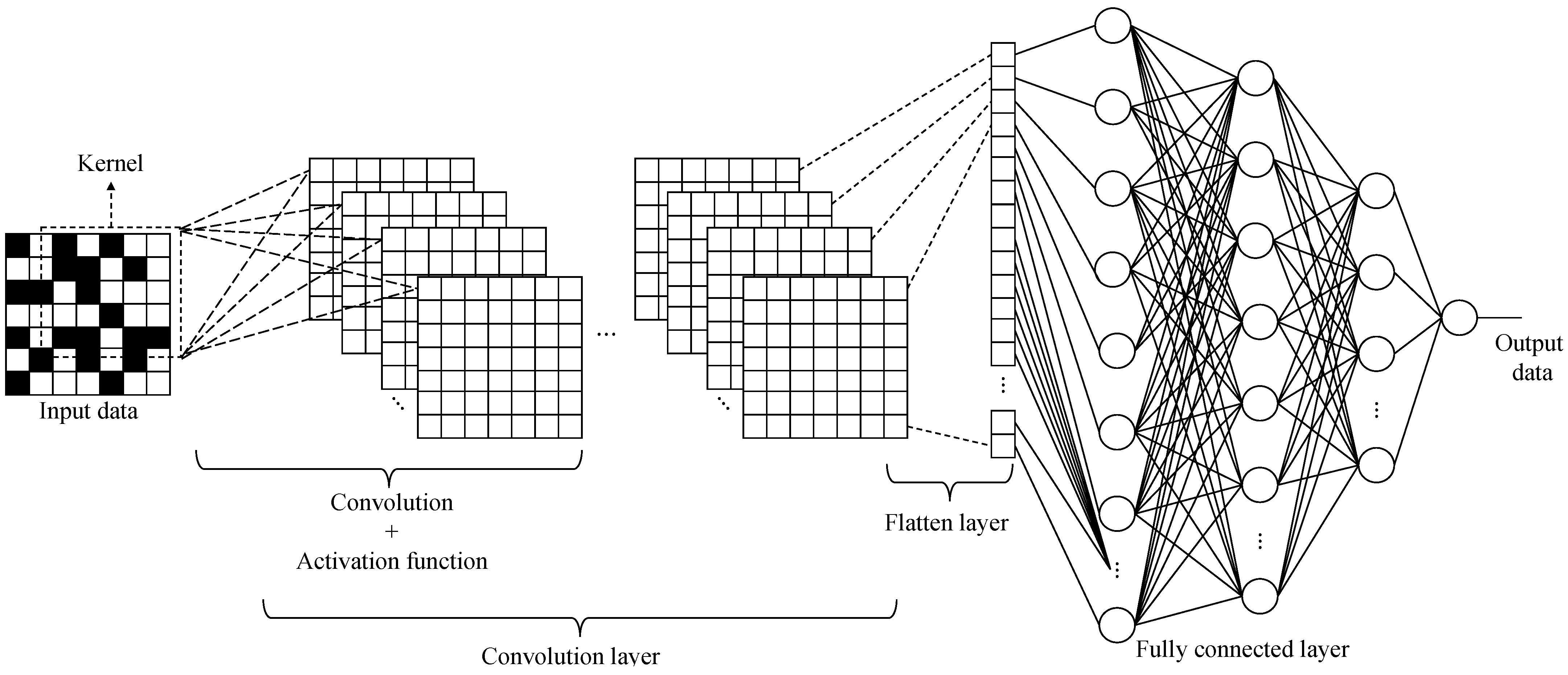
We proposed a CNN-based equalizer for the HDS systems.

-

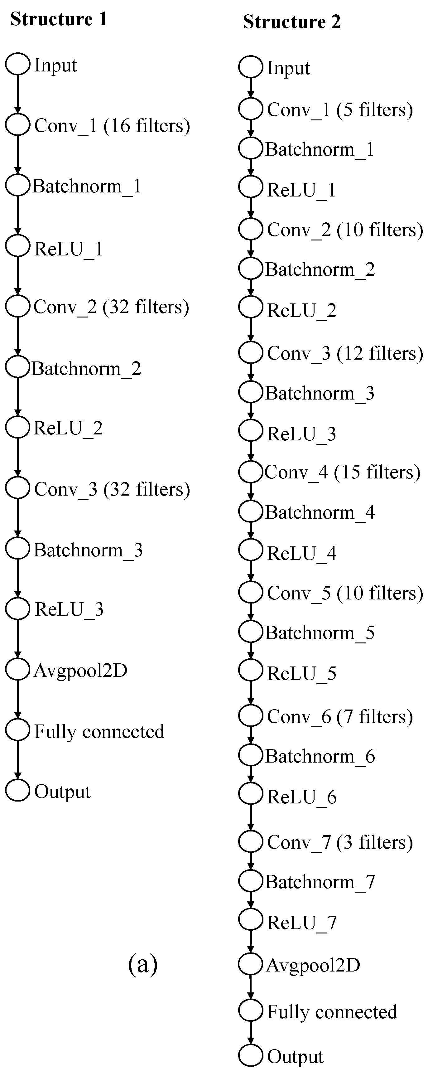
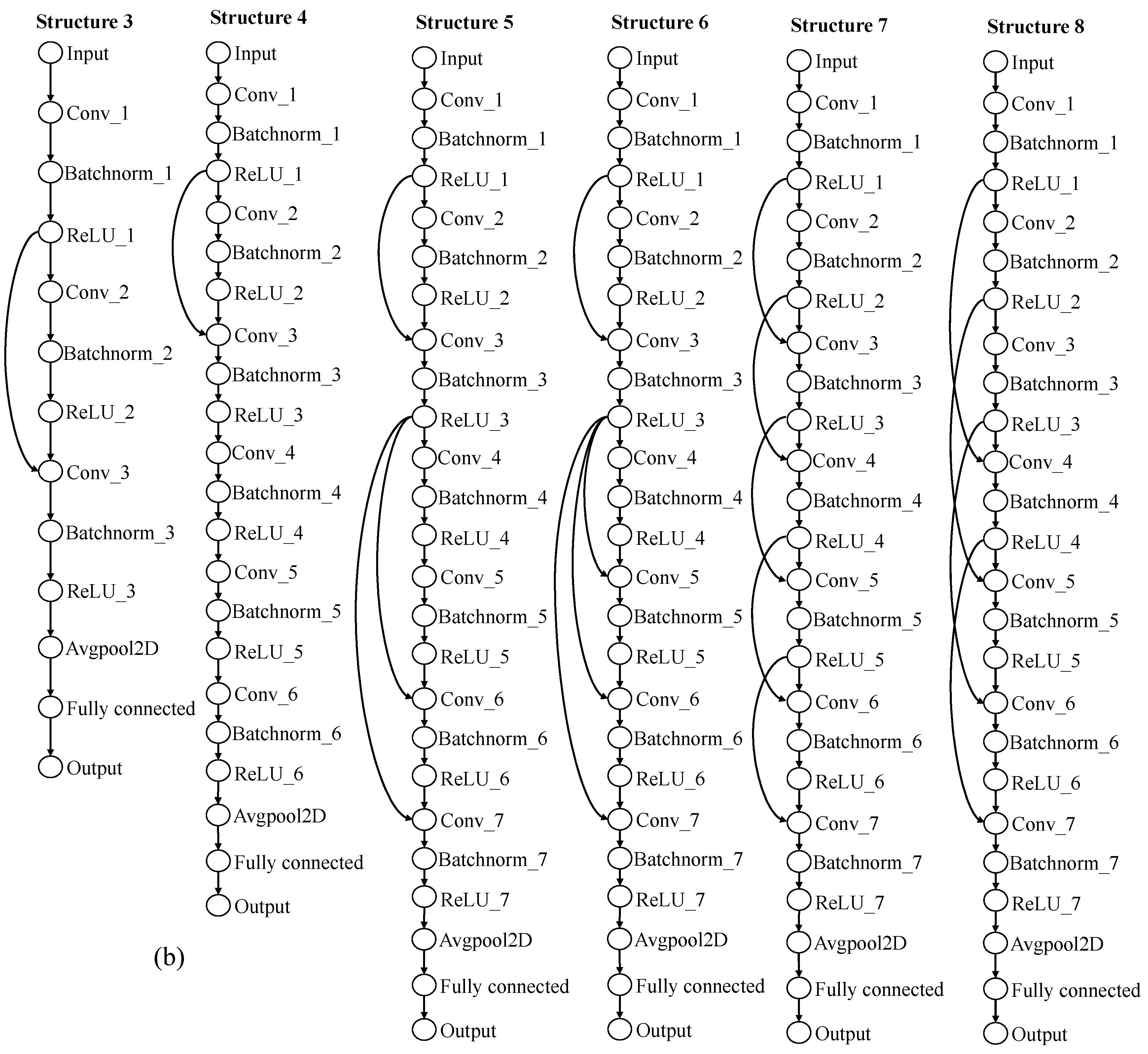
We optimized the best structure of the CNN (between straight and branch structures) for the 2D equalizer.

-

We analyzed and explained the properties of CNN structures.

-

We presented simulation results to verify the performance of the CNN-based equalizer.

The remainder of this paper is organized as follows. In Section 2, we briefly introduce the background of the equalizer and the GPR target. The channel modeling of HDS systems and the proposed scheme are presented in Section 3. Simultaneously, we also analyze and explain the properties of CNN structures in Section 3. Simulation results are presented and discussed in Section 4. The complexity and latency/delay of the proposed model are also measured in Section 4. Finally, the conclusions are presented in Section 5.

2. Background

In HDS systems, an equalizer is set up at the channel output, as shown in Figure 2.

We define the equalizer as matrix F as follows:

$$F=\left[\begin{array}{ccccc}{f}_{-2,-2}& f_{-2,-1}& f_{-2,0}& f_{-2,1}& f_{-2,2}\\ f_{-1,-2}& f_{-1,-1}& f_{-1,0}& f_{-1,1}& f_{-1,2}\\ f_{0,-2}& f_{0,-1}& f_{0,0}& f_{0,1}& f_{0,2}\\ f_{1,-2}& f_{1,-1}& f_{1,0}& f_{1,1}& f_{1,2}\\ f_{2,-2}& f_{2,-1}& f_{2,0}& f_{2,1}& f_{2,2}\end{array}\right]$$

(1)

Signal z[j,k] is calculated as follows:

$$z\left[j,k\right]={\displaystyle \sum _{n=-2}^2{\displaystyle \sum _{m=-2}^2{f}_{n,m}r\left[j-n,k-m\right]}}$$

(2)

where j and k are the indices in the horizontal and vertical directions, respectively.

To estimate the parameters f_n,m of the equalizer, we minimize the mean square error (MSE) between output signal of the equalizer z[j,k] and input signal of the channel s[j,k]. That is, this is a zero-forcing equalizer. However, because the zero-forcing equalizer is designed for 1D interference, its performance in an HDS channel is very low. In other words, signal z[j,k] cannot be approximated to signal s[j,k] in 2D ISI. Therefore, instead of approaching signal s[j,k], signal z[j,k] approaches desired signal d[j,k] in (3) by optimizing the MSE in (5) to improve the accuracy of the equalizer.

$$d\left[j,k\right]={\displaystyle \sum _{n=-1}^1{\displaystyle \sum _{m=-1}^1{t}_{n,m}s\left[j-n,k-m\right]}}$$

(3)

$$T=\left[\begin{array}{ccc}{t}_{-1,-1}& t_{-1,0}& t_{-1,1}\\ t_{0,-1}& t_{0,0}& t_{0,1}\\ t_{1,-1}& t_{1,0}& t_{1,1}\end{array}\right]$$

(4)

$$MSE=E\left\{{\left(d\left[j,k\right]-z\left[j,k\right]\right)}^2\right\}$$

(5)

If we optimize (5), the parameters for equalizer F and target T are equal to 0. Therefore, a condition is suggested to avoid F and T from being equal to 0. The condition is as follows:

$$c^{T}t=\alpha$$

(6)

where t represents a vector form of target T,

$$c^T=\left[\begin{array}{ccccccccc}0& 0& 0& 0& 1& 0& 0& 0& 0\end{array}\right], \mathrm{and}$$

(7)

$$\alpha =0.85$$

(8)

In the HDS channel, based on [19], $\alpha$ = 0.85 can be shown to achieve the best performance for the HDS channel. Applying the minimum mean square error (MMSE) algorithm, as specified in [18], the parameters for F and T can be estimated as follows:

$$t={\left(S-D^T{R}^{-1}D\right)}^{-1}c{\left(c^T{\left(S-D^T{R}^{-1}D\right)}^{-1}c\right)}^{-1}\mathsf{\alpha }, \mathrm{and}$$

(9)

$$f=R^{-1}Dt$$

(10)

Here, S = E{ss^T}, R = E{rr^T}, D = E{rs^T}, and f represents the vector form of equalizer F. s and r represent the vector forms of signals s[j,k] and r[j,k], respectively.

In the HDS channel, a point spread function (PSF) is used as the channel impulse response. Because the channel parameters far from the center are close to zero when the size is greater than a 5 × 5 array of pixels, we selected a pixel array size of 5 × 5 for the equalizer. To design a simple detection method, we selected a target size of a 3 × 3 array of pixels. This helps the trellis in horizontal and vertical detections reduce the states to only 36 and 4, respectively.

3. Proposed Model

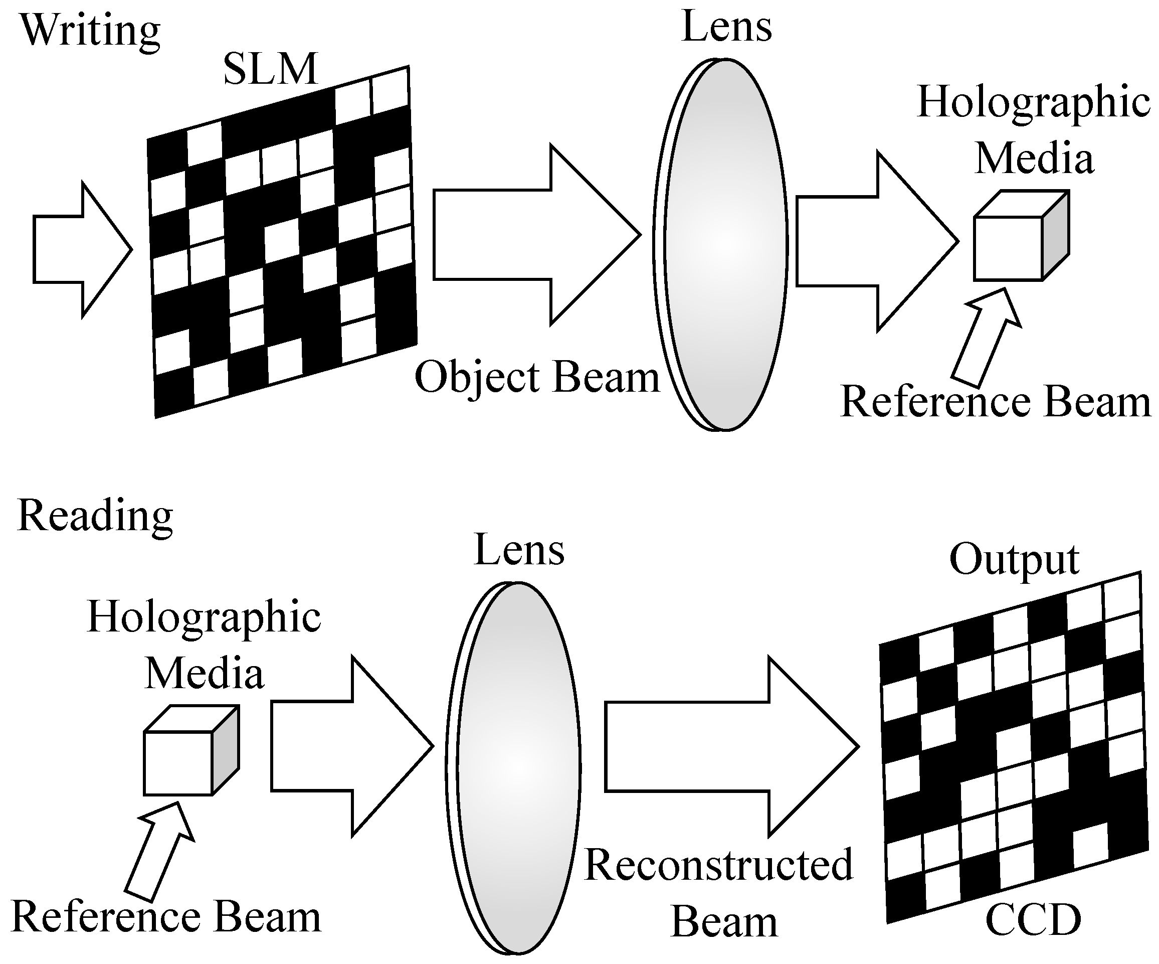
3.1. Channel Modeling

In this study, we model the HDS channel as in [14], where user signal u[k] is modulated and stored in the HDS channel as a 2D data page s[j,k]. Readback signal r[j,k] is then collected and distorted by the 2D ISI and electric noise using the following equation:

$$r\left[j,k\right]=s\left[j,k\right]\otimes H+w\left[j,k\right]$$

(11)

where $\otimes$ is the 2D convolution operator. H is a 3 $\times$ 3 matrix representing the channel impulse response of the HDS system. w[j,k] represents the white noise with the Gaussian distribution (mean zero and variance ${\sigma }_w^2$). In addition, we define the SNR as follows:

$$SNR=10{\log }_{10}\left(\frac{1}{{\sigma }_w^2}\right)$$

(12)

To obtain the parameters of H in the simulation, they are calculated from the continuous PSF as follows:

$$h_{n,m}={\displaystyle \underset{n-1/2}{\overset{n+1/2}{\int }}{\displaystyle \underset{m-1/2}{\overset{m+1/2}{\int }}h\left(x,y\right)}dxdy}$$

(13)

Here,

$$h\left(x,y\right)=\frac{1}{{\sigma }_b^2}\sin c^2\left(\frac{x-m_x}{{\sigma }_b},\frac{y-m_y}{{\sigma }_b}\right)$$

(14)

Here, sinc(x,y) = (sin($\pi$x)/$\pi$x)(sin($\pi$y)/$\pi$y); m_x denotes the misalignment in the horizontal direction; m_y denotes the misalignment in the vertical direction; and ${\sigma }_b$ denotes the blur grade. Channel matrix H has the following form:

$$H=\left[\begin{array}{ccc}{h}_{-1,-1}& h_{-1,0}& h_{-1,1}\\ h_{0,-1}& h_{0,0}& h_{0,1}\\ h_{1,-1}& h_{1,0}& h_{1,1}\end{array}\right]$$

(15)

3.2. Proposed Nonlinear Equalizer

In the conventional linear equalizer (Section 2), the 2D received signal is convoluted with only one layer (5 $\times$ 5 matrix F) from the CNN perspective. To improve the conventional equalizer, we propose a CNN structure that extends many 2D convolution layers and creates a nonlinear equalizer. CNNs are frequently proposed in the image processing field to handle 2D signals. Therefore, in the HDS channel, the CNN is suitable for the 2D received signal on the project screen. Figure 3 shows the structure of the nonlinear equalizers.

The proposed system model, based on a nonlinear CNN equalizer, is shown in Figure 4.

In our proposed model, user signal u[k] is modulated into a 2D signal s[j,k] to make it suitable for the medium of the HDS system. Signal s[j,k] is distorted by the 2D ISI and electric noise w[j,k]. Therefore, received signal r[j,k] is passed through the nonlinear equalizer (CNN) to reduce the 2D ISI and electric noise. Because of using the serial target form, signal z[j,k] can be detected using serial detection, as in [19]. Signal z[j,k] is passed through the horizontal detector to create signal b[j,k]. Signal b[j,k] is then passed through the vertical detector to restore modulated signal $\widehat{s}$[j,k]. Finally, user data u[k] are recovered by demodulating signal $\widehat{s}$[j,k]. To estimate the BER, we compare and count the difference in bits between u[k] and $\widehat{u}$[k].

In this study, we tested eight CNN structures for a nonlinear equalizer, as illustrated in Figure 5. They were grouped into two types: straight and branch structures. Straight structures are typically used in conventional CNNs. Subsequently, the branch structure of the CNN was developed to reduce the vanishing gradient phenomenon (as explained in Section 3.3). To train the CNN model, we implemented the following steps:

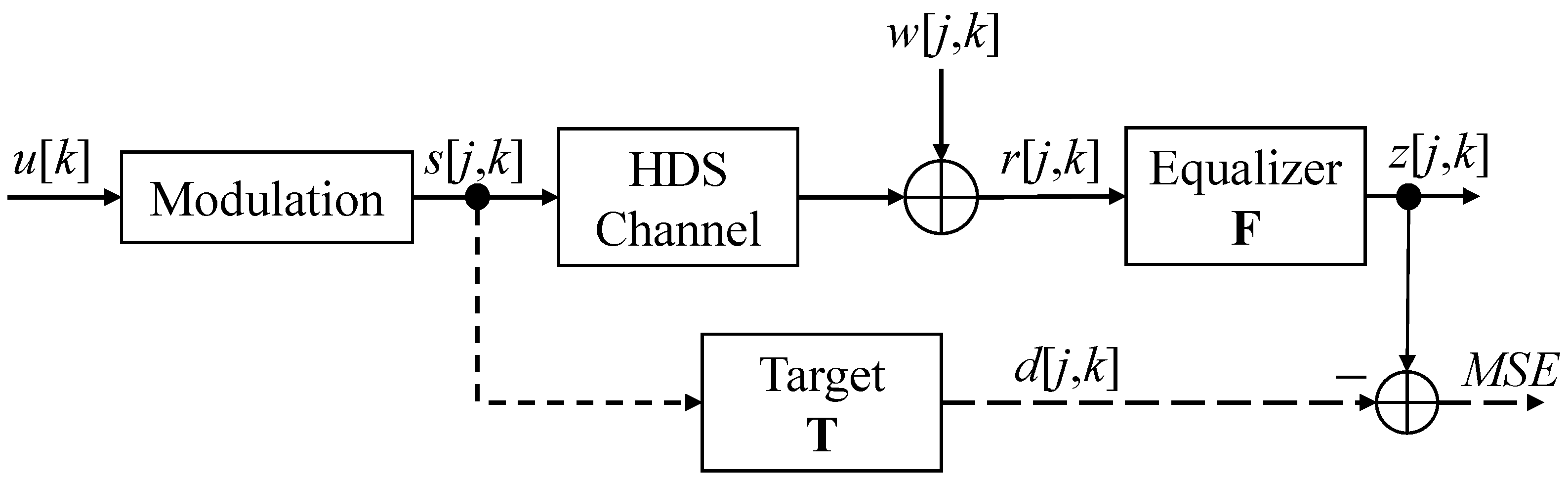
• Use MMSE algorithm, as specified in Section 2, to estimate conventional equalizer F and target T.
• Collect signals d[j,k] and r[j,k] when estimating F and T.
• Use signal r[j,k] as the input and signal d[j,k] as the label for the CNN model in the training process.
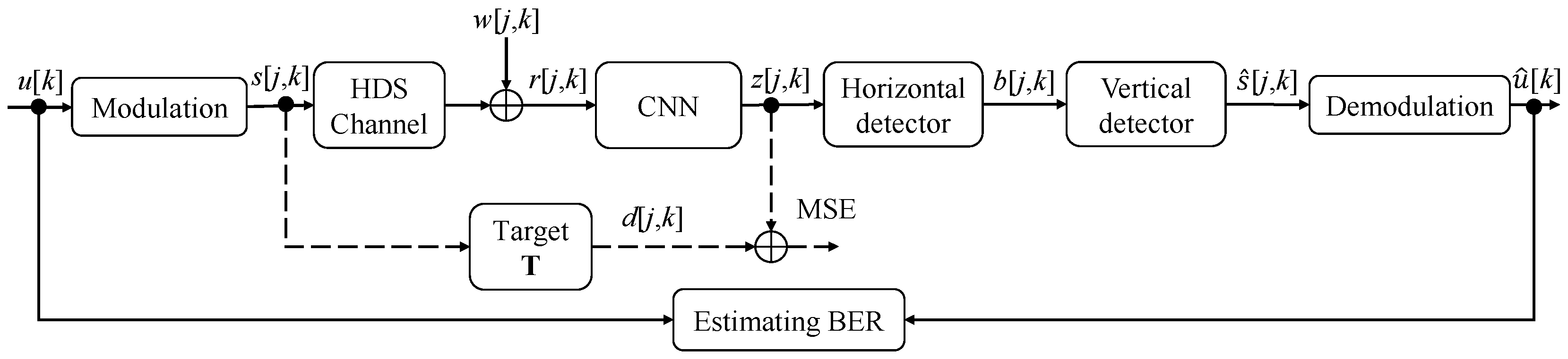
• Replace equalizer F with the trained CNN model.

In addition, we used the following MSE function as the loss function for the CNN model:

$$loss=\frac{1}{2\alpha \beta }{\displaystyle \sum _{j=1}^{\alpha }{\displaystyle \sum _{k=1}^{\beta }{\left(r\left[j,k\right]-d\left[j,k\right]\right)}^2}}$$

(16)

Here, $\alpha$ and $\beta$ represent the total number of the rows and columns of signal y[j,k], respectively.

In Figure 5, the “Conv” layers have a 5 $\times$ 5 kernel and a stride of 2 $\times$ 2. In addition, the “Avgpool2D” layers are subjected to average pooling with a size of 2 $\times$ 2 and a stride of 2 $\times$ 2. The “Batchnorm” layers used the below equation to normalize the data.

$$\widehat{x}=\frac{x-{\mu }_x}{{\sigma }_x}$$

(17)

where x is the input of “Batchnorm” layer and $\widehat{x}$ is the output of “Batchnorm” layer. ${\mu }_x$ is the mean of x, and ${\sigma }_x$ is standard deviation of x. In addition, the ReLU function is presented in (18).

$$f\left(x\right)=\{\begin{array}{c}x, x>0\\ 0, x\le 0\end{array}$$

(18)

In Figure 5b, to easily present the number of filters in “Conv” layers, we used the vector type for the number of filters as [Conv_1 Conv_2 Conv_3 …].

• Structure 3: [16 32 32].
• Structure 4: [7 10 12 15 10 7].
• Structure 5: [5 10 12 15 10 7 3].
• Structure 6: [5 10 12 15 10 7 3].
• Structure 7: [5 10 12 15 10 7 3].
• Structure 8: [5 10 12 15 10 7 3].

Based on the theory model, we can see that the CNN structure converts the received signal nonlinearly into the desired signal with a higher accuracy than the conventional equalizer structure. However, we find out that the BER performance is a little bit improved when applying the CNN structure. The reason for this problem is that when applying straight structures (Figure 5a), the weights in early layers are not updated completely. The final layers of the CNN model are trained and updated with the parameters. This is called the vanishing gradient. To solve the above problem, the skipping branch (Figure 5b) is introduced to update the parameters in early layers. Instead of the update parameters going through many layers from the final to the beginning layers, they can go directly to the early layers by skipping branches.

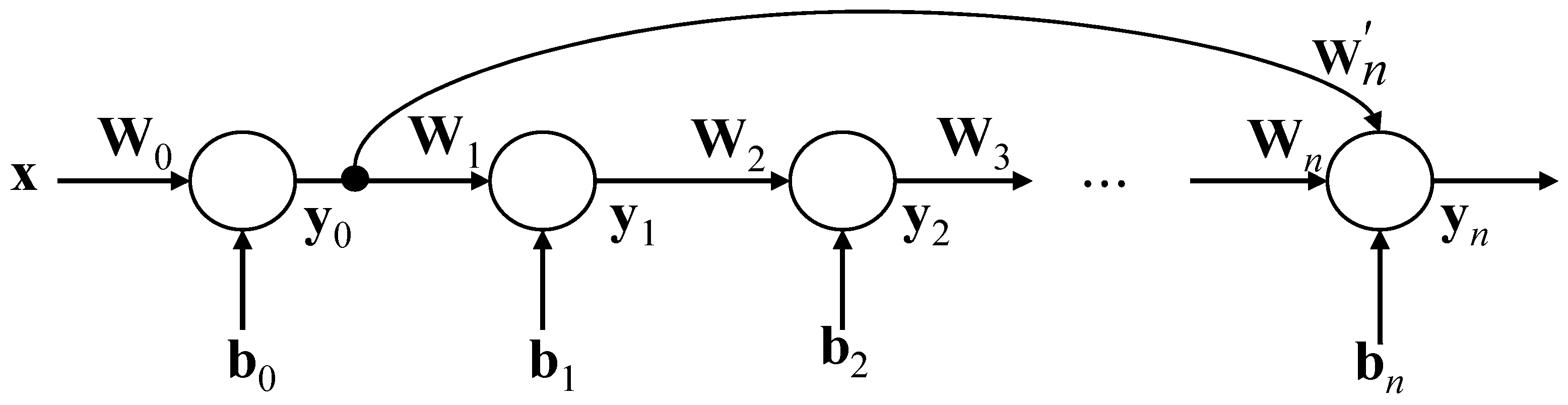
3.3. Improving CNN Equalizer with Skipping Branch

We consider the simple neural network as shown in Figure 6.

In Figure 6, the circles represent the neurons in the layers of the neural network. x denotes the input signal. W denotes the weight matrix. y denotes the output vector of each layer. b denotes the bias vector of each layer. y is calculated using the following equation:

$$y_m=f\left(W_m{y}_{m-1}+b_m\right), m=1,2,3,\dots ,n$$

(19)

With m = 0, we can use the following equation to calculate y.

$$y_0=f\left(W_{0}x+b_0\right)$$

(20)

We differentiate y_n by W₀ as follows:

$$\begin{array}{cc}\hfill \frac{\partial y_n}{\partial W_0}& =\frac{\partial f\left(W_n{y}_{n-1}+b_n\right)}{\partial \left(W_n{y}_{n-1}+b_n\right)}{W}_n\frac{\partial f\left(W_{n-1}{y}_{n-2}+b_{n-1}\right)}{\partial \left(W_{n-1}{y}_{n-2}+b_{n-1}\right)}{W}_{n-1}\dots \frac{\partial f\left(W_{0}x+b_0\right)}{\partial \left(W_{0}x+b_0\right)}x\hfill \\ & =\left[{\displaystyle \prod _{k=1}^n\frac{\partial f\left(W_k{y}_{k-1}+b_k\right)}{\partial \left(W_k{y}_{k-1}+b_k\right)}{W}_k}\right]\frac{\partial f\left(W_{0}x+b_0\right)}{\partial \left(W_{0}x+b_0\right)}x\hfill \end{array}$$

(21)

From (21), we can deduce the differentiation of y_n by W_m as follows:

$$\frac{\partial y_n}{\partial W_m}=\left[{\displaystyle \prod _{k=m}^n\frac{\partial f\left(W_k{y}_{k-1}+b_k\right)}{\partial \left(W_k{y}_{k-1}+b_k\right)}{W}_k}\right]y_{m-1}$$

(22)

According to the gradient descent algorithm, the new parameters are updated as follows:

$$W_m^{new}=W_m^{old}-\frac{\partial y_n}{\partial W_m}\epsilon$$

(23)

Here, $\epsilon$ denotes the step size or learning rate. From (22), we can observe that when the neural network has many layers to create a long network, the multiplication part ${\displaystyle \prod _{k=m}^n\frac{\partial f\left(W_k{y}_{k-1}+b_k\right)}{\partial \left(W_k{y}_{k-1}+b_k\right)}{W}_k}$ is extremely small in the beginning layers. This leads to $\frac{\partial y_n}{\partial W_m}\approx 0$ and $W_m^{new}\approx W_m^{old}$ in (23). Therefore, when the network is extremely long, we cannot exploit all the weights of all layers. This leads to a local optimized point for the network model. A skipped branch is added to the neural network structure, as shown in Figure 7.

We differentiate y_n by W₀ as follows:

$$\begin{array}{cc}\hfill \frac{\partial y_n}{\partial W_0}& =\frac{\partial f\left(W_n{y}_{n-1}+W_n^{\prime }{y}_0+b_n\right)}{\partial \left(W_n{y}_{n-1}+W_n^{\prime }{y}_0+b_n\right)}\left(W_n\frac{\partial y_{n-1}}{\partial W_0}+W_n^{\prime }\frac{\partial y_0}{\partial W_0}\right)\hfill \\ & =\frac{\partial f\left(W_n{y}_{n-1}+W_n^{\prime }{y}_0+b_n\right)}{\partial \left(W_n{y}_{n-1}+W_n^{\prime }{y}_0+b_n\right)}{W}_n\left[{\displaystyle \prod _{k=1}^{n-1}\frac{\partial f\left(W_k{y}_{k-1}+b_k\right)}{\partial \left(W_k{y}_{k-1}+b_k\right)}{W}_k}\right]\frac{\partial f\left(W_{0}x+b_0\right)}{\partial \left(W_{0}x+b_0\right)}x\hfill \\ & +\frac{\partial f\left(W_n{y}_{n-1}+W_n^{\prime }{y}_0+b_n\right)}{\partial \left(W_n{y}_{n-1}+W_n^{\prime }{y}_0+b_n\right)}{W}_n^{\prime }\frac{\partial f\left(W_{0}x+b_0\right)}{\partial \left(W_{0}x+b_0\right)}x\hfill \\ & =\left\{\left[{\displaystyle \prod _{k=1}^{n-1}\frac{\partial f\left(W_k{y}_{k-1}+b_k\right)}{\partial \left(W_k{y}_{k-1}+b_k\right)}{W}_k}\right]+W_n^{\prime }\right\}\frac{\partial f\left(W_n{y}_{n-1}+W_n^{\prime }{y}_0+b_n\right)}{\partial \left(W_n{y}_{n-1}+W_n^{\prime }{y}_0+b_n\right)}\frac{\partial f\left(W_{0}x+b_0\right)}{\partial \left(W_{0}x+b_0\right)}x\hfill \end{array}$$

(24)

From (21), we can note that multiplication part ${\displaystyle \prod _{k=m}^n\frac{\partial f\left(W_k{y}_{k-1}+b_k\right)}{\partial \left(W_k{y}_{k-1}+b_k\right)}{W}_k}$ is added to $W_n^{\prime }$. This aids $\frac{\partial y_n}{\partial W_0}>>0$, and the gradient descent can update the parameters for the beginning layers according to (23). Therefore, with the skipped branch, the neural network model can exploit all the layers and achieve a global optimized point. This is also observed in the CNN model. When an excessive number of layers are added to the CNN model, the parameters of the beginning layers cannot be updated (called the vanishing gradient). Therefore, a skipped branch is required to update the parameters of the beginning layers.

4. Simulations

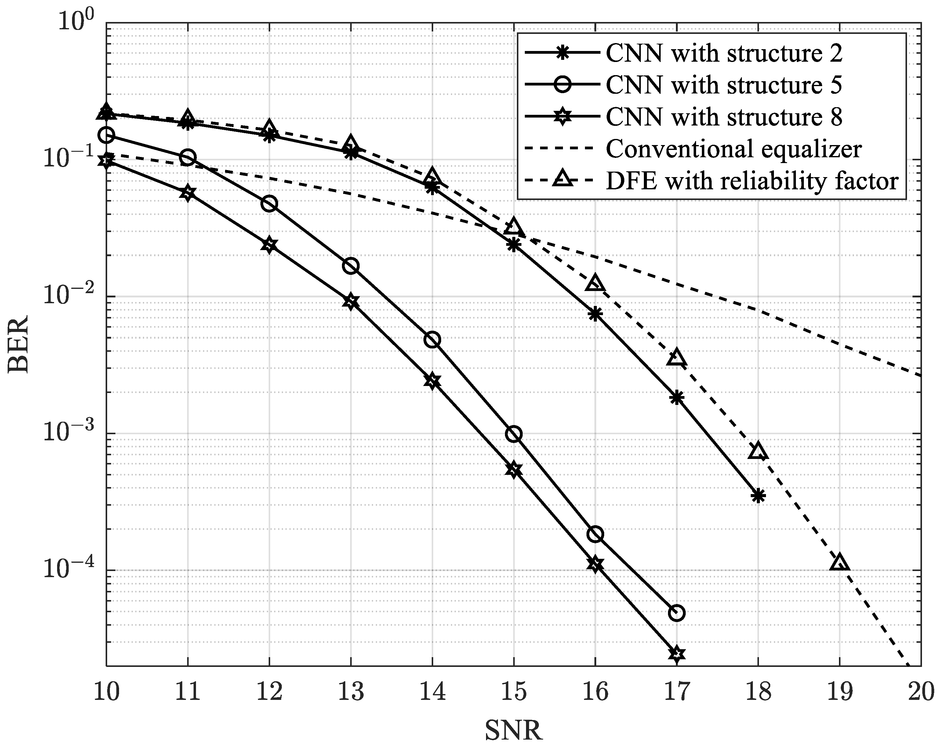
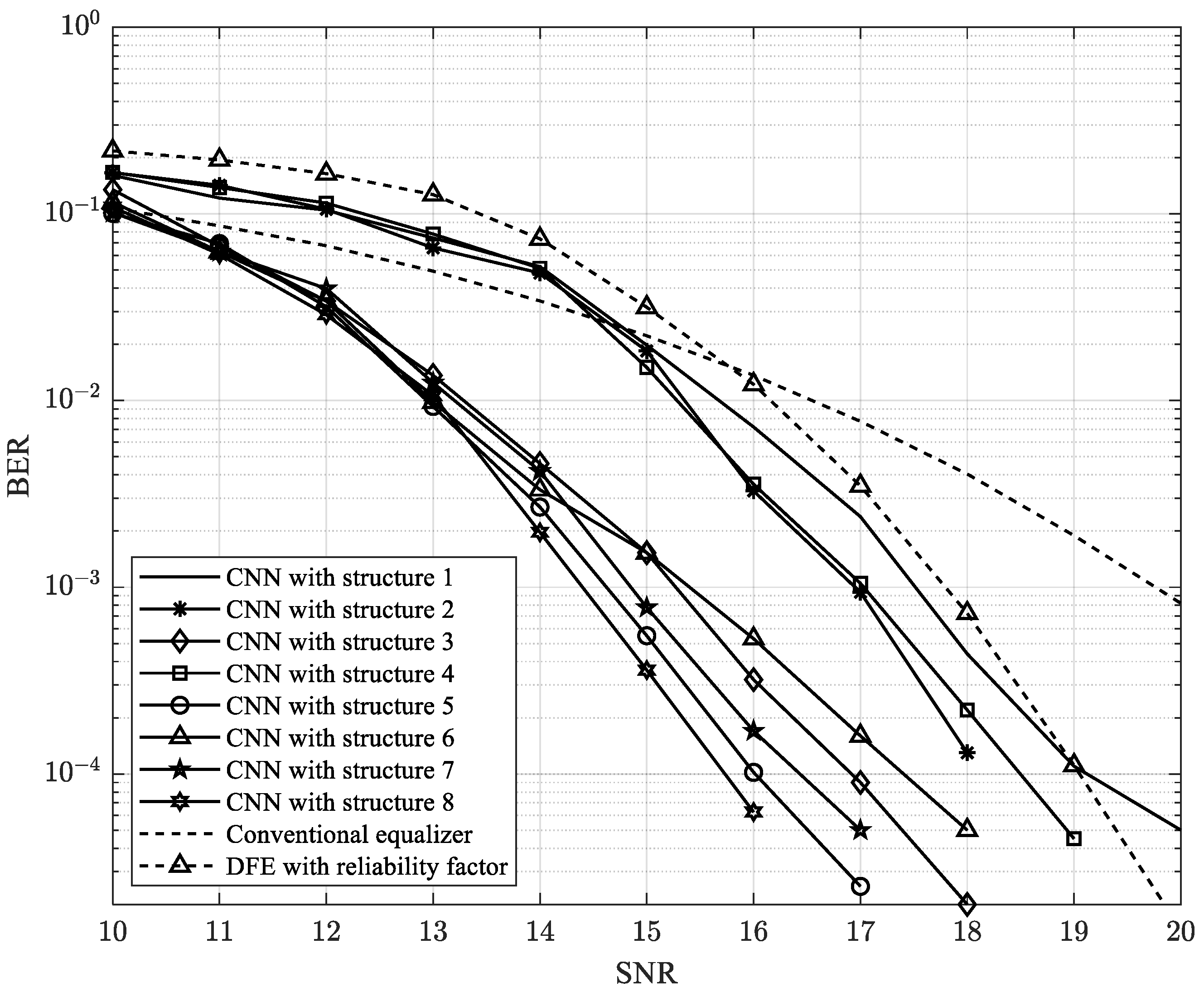
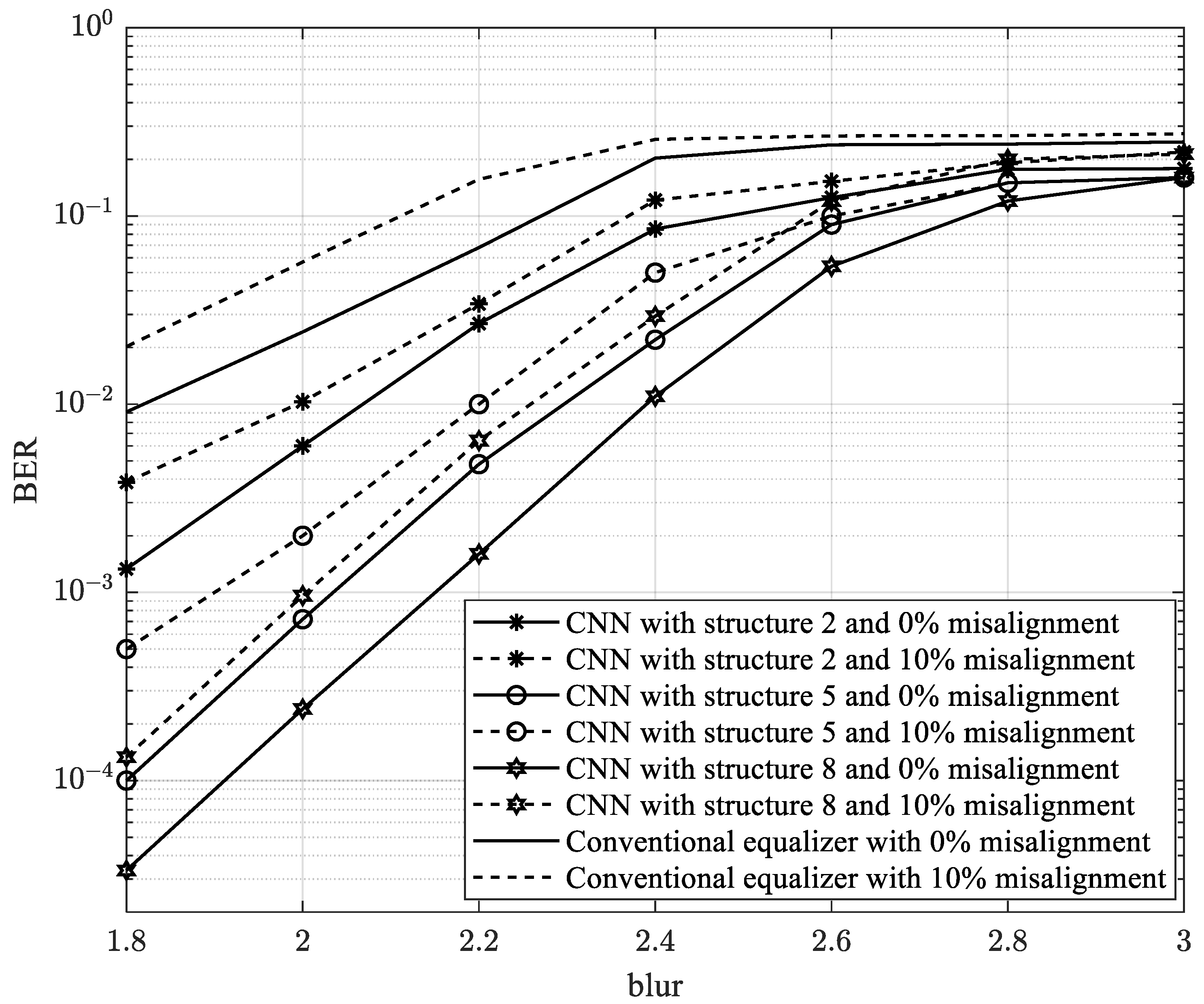
4.1. Results and Discussions

In this study, we simulated a conventional equalizer and a CNN equalizer with eight structures, as described in Section 3.2. We used a filter with a size of 5 × 5 for the convolution layers in each structure. We created a user data bit u[k] with a size of 1,440,000. Subsequently, user data u[k] were converted to signal s[j,k] with a size of 1200 $\times$ 1200 as a 2D data page via modulation. We used a data page to create signals r[j,k] and s[j,k] to estimate equalizer F and target T. Then, we created signal d[j,k] by passing signal s[j,k] through target T. We trained the CNN with signals r[j,k] and d[j,k], as described in Section 3.2. We used 20 data pages to create a dataset for training the CNN. We divided the dataset into 60% training data and 40% validation data. We set 100 epochs to train the CNN. To test the proposed model, we used 10 data pages to calculate the BER performance of the HDS channel. We used a computer with CPU i5-11400 2.6 GHz, 16 GB RAM, and a GTX 1650 graphic card. In addition, MATLAB 2023a was used to create the program. The root MSE (RMSE) results of the eight CNN structures are presented in

Table 1. The RMSE of nonlinear equalizer using CNN structures at 10 dB.

Methods	RMSE
Structure 1	0.2746
Structure 2	0.2903
Structure 3	0.2565
Structure 4	0.2477
Structure 5	0.2353
Structure 6	0.2213
Structure 7	0.2135
Structure 8	0.2047
Conventional equalizer in [18]	0.3064

.

In the first experiment, we set up an HDS channel with 0% misalignment and a blur of 1.85. The misalignment is a parameter of the HDS channel. This shows that the sensor in HDS systems is skewed towards the position of the desired data. Therefore, the misalignment effect decreased the detection ability. The blur level was a variable associated with the HDS channel. This reflected the distribution of light energy on the projection screen. As the blur level increased, more light energy was scattered in various directions, resulting in less energy being concentrated at the intended pixels and an increase in unwanted noise. This simultaneous light scattering also caused a 2D ISI to occur. Figure 8 presents the results of the first experiment.

As shown in Figure 8, the CNN equalizer could improve the BER performance compared with the conventional equalizer in [18] and the decision feedback equalizer (DFE) with a reliability factor in [2]. In addition, branch structures could achieve better performance than straight structures. However, the performance of Structure 4 was similar to that of the straight structure. Because Structure 4 has excessive layers (a long network) and the skip branch connects only to the beginning layer from the perspective of the long network, the weights were not updated completely. This led to Structure 4 and the straight structure achieving similar performance. In addition, we designed Structures 7 and 8 with skipped branches that skipped two and three layers, respectively. Notably, Structure 8 achieved a better performance than Structure 7. When Structure 8 skipped three layers, the parameter information was updated more easily than in Structure 7, with two layers skipped. In other words, Structure 8 reduced the vanishing gradient better than Structure 7. Therefore, Structure 8 improved the BER performance better than Structure 7. Generally, our proposed model achieved a gain of 3.5 dB at a BER of 10⁻³ compared to the previous model.

In the next simulation, we set blur = 1.85 and 10% misalignment for the HDS channel. The results are shown in Figure 9.

As shown in Figure 9, the proposed model could still improve the BER performance of the HDS channel. As the misalignment increases, the 2D ISI increases. Nevertheless, by employing the proposed model that considers the nonlinear connection within the CNN, we could compensate for this effect, thereby maintaining the BER performance of the HDS channel at 0% misalignment. Our proposed model obtained a gain of 2.5 dB at a BER of 10⁻³ under 10% misalignment.

In the final simulation, the blur level was changed from 1.8 to 3 with 0% and 10% misalignments. We also set SNR = 15 dB. The results are presented in Figure 10. The proposed model achieved the best performance when the blur was less than 2.8.

4.2. Complexity and Latency

In this section, we consider the complexity of our proposed model and that of previous studies in

Table 2. Complexity of our proposed model and previous studies.

Methods	Mul/Div	Add/Sub
Structure 1	1998	1955
Structure 2	4578	4435
Structure 3	2623	2555
Structure 4	4581	4438
Structure 5	6489	6271
Structure 6	7114	6871
Structure 7	7739	7471
Structure 8	7123	6817
Conventional equalizer in [18]	33	48
DFE with reliability factor [2]	>36	>34

. The operators are counted in the equalizer to detect a bit. In Table 2, we can see the trade-off between the BER performance and the complexity of the models.

In

Table 3. The processing time for eight CNN structures.

Methods	Latency (ms)
Structure 1	4.1
Structure 2	6.448
Structure 3	6.151
Structure 4	7.25
Structure 5	8.23
Structure 6	8.532
Structure 7	8.623
Structure 8	8.854
Conventional equalizer in [18]	0.0902

, we consider the processing time for each CNN structure to detect one bit. These results present the latency/delay of the proposed model.

5. Conclusions

In this study, we introduced a CNN-based equalizer designed for HDS channels. Using a pretrained CNN, we processed the received signal from the HDS channel output to mitigate the 2D ISI and achieve an equalizer output signal close to the desired target signal. In addition, we conducted experiments to determine the optimal CNN equalizer structure. The proposed equalizer demonstrated superior accuracy compared to traditional equalizers. Simulations showed that the proposed model outperformed those of prior studies. Specifically, at a BER of 10⁻³, the proposed model yielded a gain of approximately 3.5 and 2.5 dB in contrast to conventional equalizers with 0% and 10% misalignment, respectively. Furthermore, even in the presence of misalignments and blurred conditions, the proposed model consistently exhibited exceptional performance. The proposed model can resist the blur effect up to 2.8. However, our proposed model still trades off between performance and complexity/latency.

References

1. David, R.; John, G.; John, R. Data Age 2025: The Digitization of the World, from Edge to Core; IDC White Paper; Seagate: Dublin, Ireland, 2018. [Google Scholar]
2. Kim, K.; Kim, S.H.; Koo, G.; Seo, M.S.; Kim, S.W. Decision feedback equalizer for holographic data storage. Appl. Opt. 2018, 57, 4056–4066. [Google Scholar] [CrossRef]
3. Hesselink, L.; Orlov, S.S.; Bashaw, M.C. Holographic data storage systems. Proc. IEEE 2004, 92, 1231–1280. [Google Scholar] [CrossRef]
4. Wilson, W.Y.H.; Immink, K.A.S.; Xi, X.B.; Chong, T.C. Efficient coding technique for holographic storage using the method of guided scrambling. Proc. SPIE 2000, 4090, 191–196. [Google Scholar]
5. Koo, K.; Kim, S.Y.; Jeong, J.J.; Kim, S.W. Two-dimensional soft output viterbi algorithm with a variable reliability factor for holographic data storage. Jpn. J. Appl. Phys. 2013, 52, 09LE03. [Google Scholar] [CrossRef]
6. Wang, Z.; Jin, G.F.; He, Q.S.; Wu, M.X. Simultaneous defocusing of the aperture and medium on a spectroholographic storage system. Appl. Opt. 2007, 46, 5770–5778. [Google Scholar] [CrossRef]
7. Shelby, R.M.; Hoffnagle, J.A.; Burr, G.W.; Jefferson, C.M.; Bernal, M.P.; Coufal, H.; Grygier, R.K.; Gunther, H.; Macfarlane, R.M.; Sincerbox, G.T. Pixel-matched holographic data storage with megabit pages. Opt. Lett. 1997, 22, 1509–1511. [Google Scholar] [CrossRef] [PubMed]
8. Burr, G.W.; Mok, F.H.; Psaltis, D. Angle and space multiplexed holographic storage using the 90° geometry. Opt. Commun. 1995, 117, 49–55. [Google Scholar] [CrossRef]
9. Yu, F.T.; Wu, S.; Mayers, A.W.; Rajan, S. Wavelength multiplexed reflection matched spatial filters using LiNbO3. Opt. Commun. 1991, 81, 343–347. [Google Scholar] [CrossRef]
10. Rakuljic, G.A.; Leyva, V.; Yariv, A.; Yeh, P.; Gu, C. Optical data storage by using orthogonal wavelength-multiplexed volume holograms. Opt. Lett. 1992, 17, 1471–1473. [Google Scholar] [CrossRef]
11. Krile, T.F.; Hagler, M.O.; Redus, W.D.; Walkup, J.F. Multiplex holography with chirp-modulated binary phase-coded referencebeam masks. Appl. Opt. 1979, 18, 52–56. [Google Scholar] [CrossRef]
12. Ishii, N.; Katano, Y.; Muroi, T.; Kinoshita, N. Spatially coupled low-density parity-check error correction for holographic data storage. Jpn. J. Phys. 2017, 56, 09NA03. [Google Scholar] [CrossRef]
13. Cideciyan, R.; Dolivo, F.; Hermann, R.; Hirt, W.; Schott, W. A PRML system for digital magnetic recording. IEEE J. Sel. Areas Commun. 1992, 10, 38–56. [Google Scholar] [CrossRef]
14. Kim, J.; Lee, J. Two-dimensional SOVA and LDPC codes for holographic data storage system. IEEE Trans. Magn. 2009, 45, 2260–2263. [Google Scholar]
15. He, A.; Mathew, G. Nonlinear equalization for holographic data storage systems. Appl. Opt. 2006, 45, 2731–2741. [Google Scholar] [CrossRef] [PubMed]
16. Koo, K.; Kim, S.-Y.; Jeong, J.J.; Kim, S.W. Two-dimensional soft output Viterbi algorithm with dual equalizers for bit-patterned media. IEEE Trans. Magn. 2013, 49, 2555–2558. [Google Scholar] [CrossRef]
17. Kim, J.; Lee, J. Iterative two-dimensional soft output Viterbi algorithm for patterned media. IEEE Trans. Magn. 2011, 47, 594–597. [Google Scholar] [CrossRef]
18. Nabavi, S.; Kumar, B.V.K.V. Two-dimensional generalized partial response equalizer for bit-patterned media. In Proceedings of the IEEE International Conference on Communications, Glasgow, UK, 24–28 June 2007; pp. 6249–6254. [Google Scholar]
19. Nguyen, T.A.; Lee, J. Serial maximum a posteriori detection of two-dimensional generalized partial response target for holographic data storage systems. Appl. Sci. 2023, 13, 5247. [Google Scholar] [CrossRef]
20. Koo, K.; Kim, S.-Y.; Kim, S. Modified two-dimensional soft output viterbi algorithm with two-dimensional partial response target for holographic data storage. Jpn. J. Phys. 2012, 51, 08JB03. [Google Scholar] [CrossRef]
21. Koo, K.; Kim, S.-Y.; Jeong, J.; Kim, S. Data page reconstruction method based on two-dimensional soft output Viterbi algorithm with self reference for holographic data storage. Opt. Rev. 2013, 21, 591. [Google Scholar] [CrossRef]
22. Lee, S.-H.; Lim, S.-Y.; Kim, N.; Park, N.-C.; Yang, H.; Park, K.-S.; Park, Y.-P. Increasing the storage density of a page-based holographic data storage system by image upscaling using the PSF of the Nyquist aperture. Opt. Express 2011, 19, 12053––12065. [Google Scholar] [CrossRef]
23. Kim, D.-H.; Jeon, S.; Park, N.-C.; Park, K.-S. Iterative design method for an image filter to improve the bit error rate in holographic data storage systems. Microsyst. Technol. 2014, 20, 1661–1669. [Google Scholar] [CrossRef]
24. Kim, H.; Jeon, S.; Cho, J.; Kim, D.-H.; Park, N.-C. An image filter based on primary frequency analysis to improve the bit error rate in holographic data storage systems. Microsyst. Technol. 2016, 22, 1359–1365. [Google Scholar] [CrossRef]
25. Chen, C.-Y.; Fu, C.-C.; Chiueh, T.-D. Low-complexity pixel detection for images with misalignment and interpixel interference in holographic data storage. Appl. Opt. 2008, 47, 6784–6795. [Google Scholar] [CrossRef]
26. Hoang, H.A.; Yoo, M. 3ONet: 3-D Detector for Occluded Object Under Obstructed Conditions. IEEE Sens. J. 2023, 23, 18879–18892. [Google Scholar] [CrossRef]
27. Shaoshuai, S.; Zhe, W.; Jianping, S.; Xiaogang, W.; Hongsheng, L. From points to parts: 3d object detection from point cloud with part-aware and part-aggregation network. IEEE Trans. Pattern Anal. Mach. Intell. 2021, 43, 2647–2664. [Google Scholar]
28. Duong, M.-T.; Hong, M.-C. EBSD-Net: Enhancing brightness and suppressing degradation for low-light color image using deep networks. In Proceedings of the 2022 IEEE International Conference on Consumer Electronics-Asia (ICCE-Asia), Yeosu, Republic of Korea, 26–28 October 2022. [Google Scholar]
29. Wang, W.; Wu, X.; Yuan, X.; Gao, Z. An experiment-based review of low-light image enhancement methods. IEEE Access 2020, 8, 87884–87917. [Google Scholar] [CrossRef]
30. Nguyen-Vu, L.; Doan, T.-P.; Bui, M.; Hong, K.; Jung, S. On the defense of spoofing countermeasures against adversarial attacks. IEEE Access 2023, 11, 94563–94574. [Google Scholar] [CrossRef]
31. Cisse, M.M.; Adi, Y.; Neverova, N.; Keshet, J. Houdini: Fooling deep structured visual and speech recognition models with adversarial examples. Proc. Adv. Neural Inf. Process. Syst. 2017, 30, 6980–6990. [Google Scholar]
32. Jeong, S.; Lee, J. Bit-flipping scheme using k-means algorithm for bit-patterned media recording. Appl. Sci. 2022, 58, 3101704. [Google Scholar] [CrossRef]
33. Jeong, S.; Lee, J. Iterative signal detection scheme using multilayer perceptron for a bit-patterned media recording system. Appl. Sci. 2020, 10, 8819. [Google Scholar] [CrossRef]
34. Sayyafan, A.; Aboutaleb, A.; Belzel, B.J.; Sivakumar, K.; Aguilar, A.; Pinkham, C.A.; Chan, K.S.; James, A. Deep neural network media noise predictor turbo-detection system for 1-D and 2-D high-density magnetic recording. IEEE Trans. Magn. 2021, 57, 3101113. [Google Scholar] [CrossRef]
35. Shimobaba, T.; Kuwata, N.; Homma, M.; Takahashi, T.; Nagahama, Y.; Sano, M.; Hasegawa, S.; Hirayama, R.; Kakue, T.; Shiraki, A.; et al. Convolutional neural network-based data page classification for holographic memory. Appl. Opt. 2017, 56, 7327–7330. [Google Scholar] [CrossRef] [PubMed]
36. Shimobaba, T.; Endo, Y.; Hirayama, R.; Nagahama, Y.; Takahashi, T.; Nishitsuji, T.; Kakue, T.; Shiraki, A.; Takada, N.; Masuda, N.; et al. Autoencoder-based holographic image restoration. Appl. Opt. 2017, 53, F27–F30. [Google Scholar] [CrossRef] [PubMed]
37. Katano, Y.; Muroi, T.; Kinoshita, N.; Ishii, N.; Hayashi, N. Data demodulation using convolutional neural networks for holographic data storage. Jpn. J. Appl. Phys. 2018, 57, 09SC01. [Google Scholar] [CrossRef]
38. Katano, Y.; Nobukawa, T.; Muroi, T.; Kinoshita, N.; Norihiko, I. CNN-based demodulation for a complex amplitude modulation code in holographic data storage. Opt. Rev. 2021, 28, 662–672. [Google Scholar] [CrossRef]
39. Katano, Y.; Muroi, T.; Kinoshita, N.; Ishii, N. Demodulation of multi-level data using convolutional neural network in holographic data storage. In Proceedings of the 2018 Digital Image Computing: Techniques and Applications (DICTA), Canberra, ACT, Australia, 10–13 December 2018; pp. 1–5. [Google Scholar]
Figure 1. Structure of an HDS system.
Applsci 13 13029 g001
Figure 2. Equalizer and the target in an HDS system [18].
Applsci 13 13029 g002
Figure 3. Nonlinear structure for the CNN-based equalizer.
Applsci 13 13029 g003
Figure 4. Diagram of the proposed model.
Applsci 13 13029 g004
Figure 5. Structures of the CNN: (a) straight structures and (b) branch structures.
Applsci 13 13029 g005aApplsci 13 13029 g005b
Figure 6. Simple neural network structure.
Applsci 13 13029 g006
Figure 7. Neural network structure with a skipped branch.
Applsci 13 13029 g007
Figure 8. BER performance of the CNN equalizer with 1.85 blur and 0% misalignment.
Applsci 13 13029 g008
Figure 9. BER performance of the CNN equalizer with 1.85 blur and 10% misalignment.
Applsci 13 13029 g009
Figure 10. BER performance of the CNN equalizer according to blur.
Applsci 13 13029 g010