Abstract
High-resolution seismic processing involves the recovery of high-frequency components from seismic data with lower resolution. Traditional methods typically impose prior knowledge or predefined subsurface structures when modeling seismic high-resolution processes, and they are usually model-driven. Nowadays, there has been a growing utilization of deep learning techniques to enhance seismic resolution. These approaches involve feature learning from extensive training datasets through multi-layered neural networks and are fundamentally data-driven. However, the reliance on labeled data has consistently posed a primary challenge for deploying these methods in practical applications. To address this issue, a novel approach for seismic high-resolution reconstruction is introduced, employing a Cycle Generative Adversarial Neural Network (CycleGAN) trained on authentic pseudo-well data. The application of the CycleGAN involves creating dual mappings connecting low-resolution and high-resolution data. This enables the model to comprehend both the forward and inverse processes, ensuring the stability of the inverse process, particularly in the context of high-resolution reconstruction. More importantly, statistical distributions are extracted from well logs and used to randomly generate extensive sets of low-resolution and high-resolution training pairs. This training set captures the structural characteristics of the actual subsurface and leads to significant improvement of the proposed method. The results from experiments conducted on both synthetic and field examples validate the effectiveness of the proposed approach in significantly enhancing seismic resolution and achieving superior recovery of thin layers when compared with the conventional method and the deep-learning-based method.
1. Introduction
Seismic high-resolution reconstruction is a key step in processing seismic data to clearly characterize the subsurface geological structure. Owing to the band-limited characteristics inherent in raw seismic data, predicting high-resolution data is always ill-posed, resulting in several solutions applicable to the observation data. Therefore, many regularization techniques with difference operators impose the estimated high-resolution results complying with the certain distribution in terms of prior information for mitigating ill-posedness. In our opinion, regularization can mainly be divided into two categories: smooth regularization and sparse regularization. Typically, the first category considers prior knowledge by minimizing the norm of the low-order spatial derivative of the model, thus applying the results to the smooth solution [1,2]. Although this category can provide stable high-resolution data, the discontinuous geologic bodies in the results are obscured. Sparse regularization, such as the norm, can describe a blocky stratigraphic interface characterized by abrupt changes under the assumption that the strong reflectivity coefficient is sparse [3,4]. However, sparse regularization suppresses weak reflection and thin-layer structure and makes thin-layer identification difficult [5]. Therefore, many complex regularizations are designed to consider both continuous and block structures to further improve sparse solutions [6,7]. These methods often need to design complex solution systems and rely on strong empirical knowledge, resulting in poor adaptability to complex situations. To sum up, all the above regularization methods depend on the mathematical model of the specific structure (smoothness and sparsity), and these methods are referred to as model-driven methods.
In recent times, deep learning (DL) has demonstrated notable achievements in the domain of seismic data processing and interpretation [8,9,10,11,12]. Different from traditional model-driven methods, DL is a type of data-driven approach that can capture parameter characteristics and supplement additional constraints feasibly and adaptively through multiple processing layers with adjustable parameters based on a training set. Lewis and Vigh incorporate CNN-predicted prior information into the objective function of full waveform inversion, leading to the effective reconstruction of salt bodies [13]. Chen and Wang introduce a self-supervised multistep deblending framework leveraging coherence similarity, achieving accurate deblending in blended seismic acquisition [14]. Wu et al. improve seismic structural interpretation by training CNNs on synthetic seismic images generated from diverse, realistic 3D structural models [15]. Yang et al. introduce GRDNet, a fully convolutional framework featuring dense connections, designed for the efficient attenuation of ground roll noise in land seismic data, significantly improving seismic data quality [16]. However, DL’s powerful learning ability lies in its large number of optimization parameters, which leads to the need for sufficient high-quality training sets. Das et al. and Zhang et al. use the synthetic training dataset to pre-train the CNN, and then use the labeled data in the actual survey to fine-tune the pre-training network by introducing the transfer learning strategy, so as to alleviate the problem of insufficient labeled data [17,18]. Song et al. and Sang et al. use two sub-CNNs to approximate the forward and inverse processes simultaneously, and finally add unlabeled data (i.e., seismic data) to the training stage [12,19]. By adding physical constraints, the parameters of DL are further optimized and the accuracy of prediction results is improved under the condition of a limited training set [20,21].
In this paper, a data-driven framework based on deep learning aimed at improving seismic data resolution is presented. A CycleGAN is employed by us to establish bidirectional, nonlinear relationships between low- and high-resolution seismic data. This bidirectional structure not only enables us to achieve high-resolution results through inverse mapping but also ensures the fulfillment of forward mapping constraints. More importantly, aside from the training set directly generated from well logs, various reflectivity models are randomly generated based on prior information (i.e., statistical distribution) in the well logs. These models are then utilized to produce multiple pairs of seismic data with low resolution and their corresponding counterparts with enhanced resolution. This greatly expands the size and diversity of the training set, and further ensures the generalization ability and applicability of the proposed framework. Compared with the DL-based method employing an identical network architecture but without the forward mapping constraint and randomly generated datasets, the proposed method enhances the performance of seismic high-resolution reconstruction. The experiments conducted on synthetic data and field data illustrate that the proposed method can not only recover more high-frequency information but can also recover more thin layers in comparison with both the conventional method and the DL-based method.
2. Theory
2.1. Network Architecture
The generative adversarial network (GAN) is designed to learn the nonlinear mapping between the source and target domain in the game-theoretic framework. A GAN is basically composed of two parts: a generator and a discriminator. The generator outputs the synthetic data from the desired distribution, and the discriminator distinguishes whether the data are from the actual domain or produced by the generator. CycleGAN is a variant of the original GAN and consists of two GANs [22]. As shown in Figure 1a, GAN1 is designed as an inverse mapping to convert low-resolution data into high-resolution data. Accordingly, GAN2 is designed as a forward mapping to convert high-resolution data into corresponding low-resolution data. These two GANs are reverses of each other and form the bidirectional functional mappings. Benefiting from this bidirectional structure, the inverse mapping (GAN1) can obtain more stable and accurate solutions.
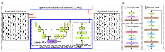
Figure 1.
(a) The framework of the CycleGAN, which includes two parts of GAN (GAN1 and GAN2). (b) The deep neural network architecture of the GAN. It is composed of three infrastructures, called the encoding block, residual block, and decoding block.
The U-shaped network as a generator, as shown in Figure 1a, consists of three parts: the encoding block, residual block, and decoding block. The feature is first down-sampled in the encoding block and then recombined with the up-sampled counterpart at each spatial resolution in the decoding block by skipping the connection. The residual block is inserted in the bottleneck of the generator to enhance the generator’s learning ability. Through three encoding blocks and one residual block, the number of feature maps is 32, 64, 128, and 256, respectively. The discriminator consists of five stacked encoding blocks, and the number of feature layers is 64, 128, 256, 512, and 1, respectively. The encoding block shown in Figure 1b includes a 3 × 1 convolutional layer with a step size of two, a LeakyReLU layer, and an Instancenormalization layer. The encoding block reduces the dimensions of seismic data and extracts their waveform characteristics. The residual block (Figure 1b) is composed of three 1 × 1 convolutional layers with a step size of one, three Instancenormalization layers, and three ReLU layers. Note that the input features of the residual block are directly added to the depth features to reduce the loss of data features, so that the network can find the best balance between accuracy and efficiency. The decoding block (Figure 1b) is composed of an upsampling layer, a 3 × 1 convolutional layer, an ReLU layer, a Dropout layer with a dropout rate of 0.2, and an Instancenormalization layer. It leverages the extracted waveform features to reconstruct seismic data. The discriminator consists of a series of encoding blocks, with a number of feature layers of 64, 128, 256, 512, and 1.
The formulated loss functions encompass two components: adversarial loss and cycle-consistent loss. Approximating the reverse transformation from low-resolution to high-resolution involves leveraging GAN1, with its adversarial loss expressed as
in which and represent the generator and discriminator of GAN1, represents the expectation operator, and and represent the low-resolution seismic data and their enhanced-resolution counterparts, as shown in Figure 1a. and describe the distributions of data associated with and . Correspondingly, the forward mapping can be approximated by GAN2
where and represent the generator and discriminator of GAN2. To make use of the knowledge contained in the forward mapping, the cycle-consistency structure is added by us to further optimize the inverse mapping, and it can be formulated as follows:
where represents the norm of the matrix. The input low-resolution trace is first fed to the in the inverse process and then outputs the estimated high-resolution result. The estimated result is fed to the to reconstruct the original low-resolution data. The cycle-consistency loss is calculated by comparing and the reconstructed low-resolution result. Similarly, the forward process uses the high-resolution trace to calculate the cycle-consistency loss. Compared with the one-way learning model (1), the cycle-consistency structure adds more loss items (3) and utilizes forward mapping to further optimize the inverse mapping . Finally, the complete loss function is defined as
where = 0.6, = 0.2, and = 0.2 are weighting parameters for controlling the training process.
2.2. Generation of the Training Set
For supervised DL methods, sufficiently large training sets that fit the characteristics of actual data are required for complex data applications. In this study, the reflectivity distribution is initially extracted based on well log data to randomly generate multiple reflectivity models. Subsequently, the non-stationary characteristics of the wavelet over time are taken into account due to the change in frequency content for generating the wavelet library. Finally, a large number of training sets are generated using the generated reflection model and wavelets with different frequency bands. This can be achieved through the following two steps:
- (1)
- Obtain the statistical distribution of the reflection coefficient based on logging data and generate multiple reflectivity models. First, we equally divide the reflection coefficient into several segments based on its valueswhere and are the maximum value and minimum value of the reflection coefficient, respectively. and are the lower and upper bounds of segment . L is the total number of segments. Then, according to the number of data points in each part, the probability is defined asin which is the number of data points in the segment , and is the total data points of the entire reflectivity. As shown in the histogram in Figure 2a, the probability is calculated with the reflection coefficient which is based on logging data (the first column in Figure 2b), where = −0.2, = 0.2, and L = 81. Finally, the Gaussian fit function is used to match the probability, and Acceptance–Rejection Sampling is used to generate a large number of reflection coefficient models that honor the extracted statistical distribution. The Gaussian fit function is expressed asin which denotes the amplitude of the Gaussian function, signifies the central position, represents the standard deviation, and n denotes the order of the Gaussian curve. Within the histogram depicted in Figure 2a, the parameters configuring the curve are established with n assigned a value of six as the Gaussian curve fits best, [, , , , , , , , , , , , , , , , , ] = [8.455, 0.00308, 0.02116, 4.751, −0.006751, 0.005758, −0.3839, −0.04897, 0.000609, 4.58, −0.01605, 0.09542, −1.403, −0.06501, 0.02489, −0.9482, −0.1161, 0.04361]. The second to fifth columns in Figure 2b show the generated reflectivity models, which are similar to the reflection coefficient (the first column) generated from actual logging data.
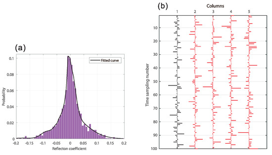 Figure 2. (a) The probability matched by the Gaussian fit function and (b) part of the randomly generated reflectivity models.
 - (2)
- Build a wavelet library with a variable frequency band and convolve it with generated reflection coefficient models. In order to alleviate the change in the frequency content of the non-stationary wavelet, the statistical wavelet is compressed and stretched through the stretch factor a by us to generate a series of wavelets with varying bandwidths. This process can be formulated as follows:in which w and are the original wavelet and the wavelet changed by a stretch factor a in the time domain, respectively, and W and are their Fourier transforms. The peak frequency range of the low-frequency wavelet is 0.7–1.4 times the main frequency of the original data, and the corresponding high-frequency wavelet is generated according to the bandwidth factor (a = 2.5). Finally, the generated low- and high-frequency wavelet pairs are convolved with the reflection coefficient model to generate corresponding low- and high-frequency traces, as shown in Figure 1a.
3. Examples
In this section, the efficacy of our proposed method is showcased through a comparative analysis with the model-driven method (sparse spike inversion [4]) and the DL-based method. The DL-based method employs an identical neural network architecture to our proposed method but lacks randomly generated datasets and the cycle-consistency loss (i.e., = = 0). In addition, the pairs of seismic traces are cropped into small patches for data augmentation, with the size of each patch set at 96 × 1. The Adam optimizer is used to update the network parameters with a learning rate of 0.001. Compared with the sparse spike inversion (SSI) and the DL-based method, more accurate high-resolution results can be obtained through our method.
3.1. Synthetic Example
The generated synthetic seismic data result from convolving a 20 Hz Ricker wavelet with the reflection coefficient model (Figure 3a) and introducing 15% random noise (i.e., the S/N is 15 dB). Figure 3b shows the synthetic seismic data, including 1400 traces, each of which has a 2440 time sampling number. The trace located at common middle point (CDP) 700 is selected as a pseudo well, whose true reflection coefficient is already known, to calculate the statistical distribution and randomly generate multiple reflection coefficient models. The 20 Hz Ricker wavelet is used as a statistical wavelet to build the wavelet library, and the 50 Hz Ricker wavelet is convolved with the reflection model (Figure 4a) to generate the true high-resolution data (Figure 3d). Figure 3a–c show three high-resolution results using SSI, the DL-based method, and the proposed method, respectively. From the results, it is evident that the high-resolution estimate in Figure 3c reveals weaker reflectivity and exhibits greater resemblance to the actual high-resolution data (Figure 3d) compared with other methods. Figure 5a–c illustrates the respective reconstruction errors between the high-resolution results and the true data. Analyzing the reconstruction error reveals that, in most instances, the high-resolution data obtained using the proposed method (Figure 5c) exhibit lower errors compared with other methods.
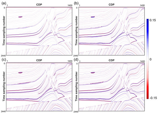
Figure 3.
Contrasts among the inferred high-resolution results are illustrated in (a–c) for SSI, the DL-based method, and the proposed method, respectively. (d) Represents the true high-resolution data.
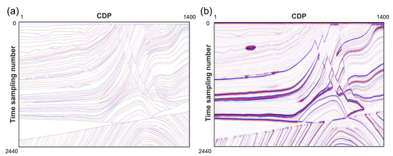
Figure 4.
Synthetic example of the high-resolution reconstruction. (a) The reflection coefficient model. (b) The synthetic seismic data (S/N = 15.0).
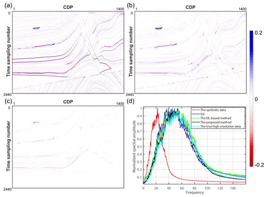
Figure 5.
(a–c) Reconstructed errors for SSI, the DL-based method, and the proposed method, respectively. (d) Amplitude spectrum comparison of the synthetic data, outcomes from SSI, the DL-based method, and the proposed method, as well as the true high-resolution data.
Additionally, Figure 5d depicts the normalized amplitude spectrum (AMP) of synthetic data, SSI, the DL-based method, the proposed method, and the true high-resolution data. Clearly, the outcome achieved by the proposed method (indicated by the black line) aligns more closely with the true high-resolution data (represented by the cyan line).
3.2. Field Data Example
A stacked seismic dataset from East China (Figure 6a) is used to thoroughly examine the effectiveness and applicability of the proposed method. The 2D field data comprise 200 seismic traces in the lateral direction, with each trace containing 700 sampling points spaced at intervals of 2 ms. Notably, there are two wells in these data, situated at CDPs of 32 and 68. The former well is employed for extracting the reflection coefficient distribution and generating a substantial number of reflection coefficients, while the latter serves as a blind well to assess the accuracy of the results.
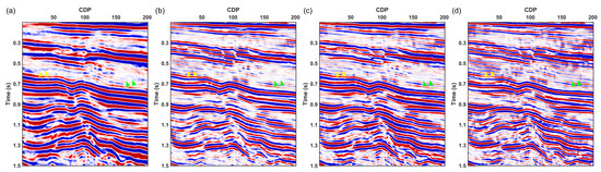
Figure 6.
Comparison of the high-resolution results. (a) Field data. (b–d) High-resolution results of SSI, the DL-based method, and the proposed method, respectively. The proposed method can better restore thin layers and yield more consistent horizontal high-resolution results (yellow and green arrows).
Furthermore, the statistical methodology within Hampson-Russell software is employed by us to extract the wavelet and construct the low-frequency wavelet library. The high-resolution results of SSI, the DL-based method, and the proposed method are presented in Figure 6b–d. It can be seen that the weak reflection and thin-layer structure are efficiently recovered by the proposed method compared with other methods, especially as indicated by the arrow. In Figure 7, the amplitude spectrum (AMP) of the output illustrates that the proposed method reconstructs a broader frequency range, where the high-frequency component distinctly exceeds that of other methods.
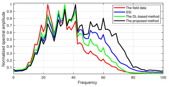
Figure 7.
The AMP of the field data, the result from SSI, the DL-based method, and the proposed method, respectively.
A comprehensive comparison between the validation data derived from well-log reflectivity and the inverted high-resolution results is depicted in Figure 8. The 2-6-60-90 Hz bandpass filter is used to generate the validation data to evaluate the accuracy of the inverted results. Apparent in Figure 8 is the effectiveness of the proposed approach (the black curve), displaying not only a strong agreement with the verification data (the red curve) concerning robust amplitudes but also a precise retrieval of weaker amplitudes, including those within the amplification segment. The Pearson correlation coefficient (PCC) of the reconstructed high-resolution data on the blind well is also compared by us. The calculated PCC values of SSI, the DL-based method, and the proposed method are 0.7495, 0.7114, and 0.8012, respectively. It can be concluded that the high-resolution result of our method coincides with the validation data the whole time.
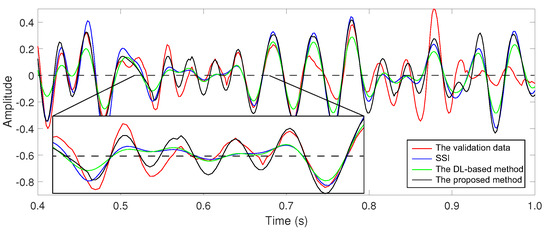
Figure 8.
Comparison of different data corresponding to the validation data.
4. Conclusions
In this letter, a data-driven framework based on DL is proposed by us to establish bidirectional mappings, namely forward mapping and inverse mapping, with the aim of enhancing seismic resolution. The proposed method has two important advantages. First, the CycleGAN network is used to build a DL-based seismic high-resolution reconstruction workflow, which directly implements feature learning and forms a nonlinear inverse mapping without the need for assumptions as in the traditional methods. In addition, benefiting from the bidirectional mappings architecture, the CycleGAN-based method facilitates the inverse problems while honoring forward mapping constraints. Second, the characteristics of seismic data, including reflectivity distribution and wavelet attributes, are utilized for the generation of extensive training sets. This augmentation significantly enhances the performance of the proposed method in processing seismic data. The synthetic and field data illustrations affirm the capability of the proposed method to enhance seismic resolution effectively and accurately reconstruct thin-layer structures, distinguishing it from the conventional method and the DL-based method.
Author Contributions
Conceptualization, X.Z. and Y.G.; methodology, W.G.; software, Y.G.; validation, X.Z., Y.G. and S.G.; formal analysis, G.L. and W.G.; investigation, X.Z. and S.G.; writing—original draft preparation, Y.G.; writing—review and editing, X.Z. and Y.G.; visualization, W.G.; supervision, G.L. and Y.G.; project administration, X.Z.; funding acquisition, X.Z. and G.L. All authors have read and agreed to the published version of the manuscript.
Funding
This research was funded by the National Key R&D Program of China (2018YFA0702504) and the Fundamental Research Project of CNPC Geophysical Key Lab (2022DQ0604-4).
Institutional Review Board Statement
Not applicable.
Informed Consent Statement
Not applicable.
Data Availability Statement
The data presented in this study are available on request from the corresponding author. The data are not publicly available due our projects are confidential.
Acknowledgments
The authors would like to thank Z. Zheng, J. Xu, and S. Zhang for constructive discussions.
Conflicts of Interest
The authors declare no conflict of interest.
References
- Berkhout, A. Least-squares inverse filtering and wavelet deconvolution. Geophysics 1977, 42, 1369–1383. [Google Scholar] [CrossRef]
- Walker, C.; Ulrych, T.J. Autoregressive recovery of the acoustic impedance. Geophysics 1983, 48, 1338–1350. [Google Scholar] [CrossRef]
- Ooe, M.; Ulrych, T. Minimum entropy deconvolution with an exponential transformation. Geophys. Prospect. 1979, 27, 458–473. [Google Scholar] [CrossRef]
- Sacchi, M.D. Reweighting strategies in seismic deconvolution. Geophys. J. Int. 1997, 129, 651–656. [Google Scholar] [CrossRef]
- Wang, Y.; Zhang, G.; Li, H.; Yang, W.; Wang, W. The high-resolution seismic deconvolution method based on joint sparse representation using logging–seismic data. Geophys. Prospect. 2022, 70, 1313–1326. [Google Scholar] [CrossRef]
- Charbonnier, P.; Blanc-Féraud, L.; Aubert, G.; Barlaud, M. Deterministic edge-preserving regularization in computed imaging. IEEE Trans. Image Process. 1997, 6, 298–311. [Google Scholar] [CrossRef]
- Kazemi, N.; Bongajum, E.; Sacchi, M.D. Surface-consistent sparse multichannel blind deconvolution of seismic signals. IEEE Trans. Geosci. Remote. Sens. 2016, 54, 3200–3207. [Google Scholar] [CrossRef]
- Wu, X.; Liang, L.; Shi, Y.; Fomel, S. FaultSeg3D: Using synthetic data sets to train an end-to-end convolutional neural network for 3D seismic fault segmentation. Geophysics 2019, 84, IM35–IM45. [Google Scholar] [CrossRef]
- Chen, W.; Yang, L.; Zha, B.; Zhang, M.; Chen, Y. Deep learning reservoir porosity prediction based on multilayer long short-term memory network. Geophysics 2020, 85, WA213–WA225. [Google Scholar] [CrossRef]
- Wang, Y.; Qiu, Q.; Lan, Z.; Chen, K.; Zhou, J.; Gao, P.; Zhang, W. Identifying microseismic events using a dual-channel CNN with wavelet packets decomposition coefficients. Comput. Geosci. 2022, 166, 105164. [Google Scholar] [CrossRef]
- Yang, L.; Wang, S.; Chen, X.; Chen, W.; Saad, O.M.; Zhou, X.; Pham, N.; Geng, Z.; Fomel, S.; Chen, Y. High-fidelity permeability and porosity prediction using deep learning with the self-attention mechanism. IEEE Trans. Neural Netw. Learn. Syst. 2022, 34, 3429–3443. [Google Scholar] [CrossRef] [PubMed]
- Sang, W.; Yuan, S.; Han, H.; Liu, H.; Yu, Y. Porosity prediction using semi-supervised learning with biased well log data for improving estimation accuracy and reducing prediction uncertainty. Geophys. J. Int. 2023, 232, 940–957. [Google Scholar] [CrossRef]
- Lewis, W.; Vigh, D. Deep learning prior models from seismic images for full-waveform inversion. In Proceedings of the SEG International Exposition and Annual Meeting, SEG, Houston, TX, USA, 24–29 September 2017; p. SEG-2017. [Google Scholar]
- Chen, X.; Wang, B. Self-supervised Multistep Seismic Data Deblending. Surv. Geophys. 2023, 1–25. [Google Scholar] [CrossRef]
- Wu, X.; Geng, Z.; Shi, Y.; Pham, N.; Fomel, S.; Caumon, G. Building realistic structure models to train convolutional neural networks for seismic structural interpretation. Geophysics 2020, 85, WA27–WA39. [Google Scholar] [CrossRef]
- Yang, L.; Wang, S.; Chen, X.; Saad, O.M.; Cheng, W.; Chen, Y. Deep Learning with Fully Convolutional and Dense Connection Framework for Ground Roll Attenuation. Surv. Geophys. 2023, 44, 1919–1952. [Google Scholar] [CrossRef]
- Das, V.; Pollack, A.; Wollner, U.; Mukerji, T. Convolutional neural network for seismic impedance inversion. In Proceedings of the 2018 SEG International Exposition and Annual Meeting, OnePetro, Anaheim, CA, USA, 14–19 October 2018. [Google Scholar]
- Zhang, J.; Li, J.; Chen, X.; Li, Y.; Huang, G.; Chen, Y. Robust deep learning seismic inversion with a priori initial model constraint. Geophys. J. Int. 2021, 225, 2001–2019. [Google Scholar] [CrossRef]
- Song, C.; Lu, W.; Wang, Y.; Jin, S.; Tang, J.; Chen, L. Reservoir Prediction Based on Closed-Loop CNN and Virtual Well-Logging Labels. IEEE Trans. Geosci. Remote. Sens. 2022, 60, 5919912. [Google Scholar] [CrossRef]
- Wang, Y.; Wang, Q.; Lu, W.; Li, H. Physics-Constrained Seismic Impedance Inversion Based on Deep Learning. IEEE Geosci. Remote. Sens. Lett. 2021, 19, 7503305. [Google Scholar] [CrossRef]
- Gao, Y.; Zhang, J.; Li, H.; Li, G. Incorporating Structural Constraint Into the Machine Learning High-Resolution Seismic Reconstruction. IEEE Trans. Geosci. Remote. Sens. 2022, 60, 5912712. [Google Scholar] [CrossRef]
- Isola, P.; Zhu, J.Y.; Zhou, T.; Efros, A.A. Image-to-image translation with conditional adversarial networks. In Proceedings of the IEEE Conference on Computer Vision and Pattern Recognition, Honolulu, HI, USA, 21–26 July 2017; pp. 1125–1134. [Google Scholar]
Disclaimer/Publisher’s Note: The statements, opinions and data contained in all publications are solely those of the individual author(s) and contributor(s) and not of MDPI and/or the editor(s). MDPI and/or the editor(s) disclaim responsibility for any injury to people or property resulting from any ideas, methods, instructions or products referred to in the content. |
© 2023 by the authors. Licensee MDPI, Basel, Switzerland. This article is an open access article distributed under the terms and conditions of the Creative Commons Attribution (CC BY) license (https://creativecommons.org/licenses/by/4.0/).