Estimation of Daily Actual Evapotranspiration of Tea Plantations Using Ensemble Machine Learning Algorithms and Six Available Scenarios of Meteorological Data

Abstract

The tea plant (Camellia sinensis), as a major, global cash crop providing beverages, is facing major challenges from droughts and water shortages due to climate change. The accurate estimation of the actual evapotranspiration (ET_a) of tea plants is essential for improving the water management and crop health of tea plantations. However, an accurate quantification of tea plantations’ ET_a is lacking due to the complex and non-linear process that is difficult to measure and estimate accurately. Ensemble learning (EL) is a promising potential algorithm for accurate evapotranspiration prediction, which solves this complexity through the new field of machine learning. In this study, we investigated the potential of three EL algorithms—random forest (RF), bagging, and adaptive boosting (Ad)—for predicting the daily ET_a of tea plants, which were then compared with the commonly used k-nearest neighbor (KNN), support vector machine (SVM), and multilayer perceptron (MLP) algorithms, and the experimental model. We used 36 estimation models with six scenarios from available meteorological and evapotranspiration data collected from tea plantations over a period of 12 years (2010–2021). The results show that the combination of R_n (net radiation), T_mean (mean air temperature), and RH (relative humidity) achieved reasonable precision in assessing the daily ET_a of tea plantations in the absence of climatic datasets. Compared with other advanced models, the RF model demonstrated superior performance (root mean square error (RMSE): 0.41–0.56 mm day⁻¹, mean absolute error (MAE): 0.32–0.42 mm day⁻¹, R²: 0.84–0.91) in predicting the daily ET_a of tea plantations, except in Scenario 6, followed by the bagging, SVM, KNN, Ad, and MLP algorithms. In addition, the RF and bagging models exhibited the highest steadiness with low RMSE values increasing (−15.3~+18.5%) in the validation phase over the testing phase. Considering the high prediction accuracy and stability of the studied models, the RF and bagging models can be recommended for estimating the daily ET_a estimation of tea plantations. The importance analysis from the studied models demonstrated that the R_n and T_mean are the most critical influential variables that affect the observed and predicted daily ET_a dynamics of tea plantations.

1. Introduction

The tea plant (Camellia sinensis) is one of the most important beverage crops in the world, covering a total area of 21.1 million ha in 2016 [1]. In China, tea plants are planted on about 3.02 million ha of land, accounting for 14.3% of the global planting area [2]. The tea plant is tolerant of shade and humidity but sensitive to water stress [3]. A lack of water, even for a short time, will affect the growth and production of tea plants, resulting in a significant yield reduction [4]. Tea plantations in China are generally located in humid subtropical and tropical regions, where the rainfall is sufficient to meet the demands of the tea plants [5]. Tea is a rain-fed crop, and thus, refined irrigation scheduling is rarely practiced in tea plantations in China [6,7]. However, the frequency of drought and extreme precipitation events has increased considerably with global climate warming, and tea plantations in China are facing major challenges, such as crop health and a decrease in agricultural yield, due to droughts and water shortages [8,9,10]. The actual evapotranspiration (ET_a) is an essential variable in the hydrological cycle, particularly for the optimization of water use and the management of tea plantations. Therefore, the accurate estimation of tea plantation ET_a is essential for improving water management, crop health, and agricultural yield in tea plantations.

Different methods and techniques have been used to measure or estimate ET_a. Measurement techniques for ET_a include the use of weighing lysimeters, soil water measurement, eddy covariance, the Bowen ratio, and large-aperture scintillometers [11,12,13,14]. Among them, the weighing lysimeters and soil water measurements for obtaining the ET_a of ecosystems are based on the water balance principle [15,16]. The eddy covariance, Bowen ratio, and large-aperture scintillometer are based on the surface energy balance and turbulent flux exchange in the atmosphere and the vegetation interface [17,18,19,20,21]. These methods have been proven effective for ET_a measurement. However, the installation and maintenance of these instruments and equipment are expensive. Meanwhile, these methods also exhibit significant spatial and temporal limitations, with multiple sources of errors arising from the extensive measurements and data elaboration, which limit the reliability and transportability of the ET_a measurement results [6,22]. Various models have also been proposed for ET_a estimation. The Penman–Monteith (P-M) equation is one of the most commonly used methods for evaluating ET_a on the basis of meteorological and biological variables [23,24]. Compared with other models, the P-M equation, which considers the energy balance and aerodynamic principles, exhibits high superiority in different ecosystems and under varying climatic conditions [13,25]. However, massive meteorological variables including air temperature, wind speed, surface heat flux, solar radiation, and relative humidity are required for ET_a estimation based on the P–M equation. This condition restricts the application of this model due to the availability and/or questionable quality of data from weather stations.

As alternatives to the aforementioned methods, various machine learning algorithms have been applied to the estimation of ET_a. These algorithms are more economical and require fewer variables as input. Granata et al. (2020) employed random forest (RF), multilayer perceptron (MLP), and k-nearest neighbor (KNN) to forecast the ET_a for a subtropical wetland. Artificial neural network (ANN) and support vector machine (SVM) models were implemented by [26] for estimating rain-fed maize field evapotranspiration. Hu et al. (2021b) used a deep neural network, RF, and symbolic regression to estimate evapotranspiration using meteorological and plant data. These attempts have proven that machine learning methods are effective tools for accurate evapotranspiration estimation [27,28,29]. In particular, the tree-based ensemble model exhibits high superiority in ET_a estimations for multiple ecosystems in different climatic regions [30,31,32,33]. However, to the authors’ limited knowledge, there are no machine learning algorithms that have been used to predict the ET_a in tea plantations. Hence, as the world’s largest tea-plant-producing country, developing advanced machine learning models for estimating with high accuracy the ET_a in tea plantations is a necessity in China.

In this study, we select three EL machine learning algorithms (RF, bagging, and Ad) and three conventional machine learning algorithms (KNN, SVM, and MLP) to estimate the daily ET_a of tea plantations by using the available tea plantations’ meteorological and evapotranspiration data collected over 12 years (2010–2021). The primary objective of this study is to investigate the potential of ensemble machine learning algorithms for estimating the ET_a in tea plantations. Moreover, we examine the accuracy of model changes with multiple variable scenarios and identify the key data-driven factors for the estimation of tea plantation ET_a. EL algorithms, such as the bagging and Ad models, are seldom employed in ET_a estimations. Considering the superiority of the tree-based ensemble model in ET_a estimations, we hypothesized that the bagging and Ad models can achieve a high performance similar to that of the RF model.

2. Materials and Methods

2.1. Study Area Description

Our study area (Tianmu Lake catchment (Figure 1c)), positioned in southeast China, is placed in the western headwater region of Taihu Lake Basin (Figure 1). It enjoys a subtropical monsoon climate characterized by 2 major rainy seasons (April to September) and a dry season (October to March). Annual precipitation and average air temperature are 1147 mm and 15.8 °C, respectively. The precipitation in the rainy season accounts for 75% of the annual total precipitation, and the lowest and highest temperatures occur in January (3.1 °C) and July (28.4 °C), respectively. Tianmu Lake catchment has also experienced rapid tea plantation expansion accompanied by dramatic land use cover changes in the last two decades (Figure 1). The area of tea plantations obviously increased from 2006 to 2013, reaching 28.6 km² in 2013, accounting for 11.7% of the catchment area. Although Tianmu Lake catchment experiences a sub-tropical climate, drought occurs frequently in the growing season. Hence, it is vital to develop accurate ET_a estimations for crop water management in the tea plantations. In our study area, the tea plantations are planted with a density of 45,000 plants ha⁻¹ with an inter-row spacing of 1.5 m. Figure 1 and

Table 1. Weather and eddy covariance flux site information (MAP: mean annual precipitation; MAT: mean annual temperature).

Name	Longitude	Latitude	Elevation (m)	MAP (mm)	MAT (°C)	Period	LULC
SSY	119.316	31.268	55	1249.3	15.8	2010–2017	3–10 years old tea
TMXM	119.397	31.313	39	1507.4	17.8	2020–2021	5–6 years old tea
TMHS	119.411	31.269	28	1371.3	16.7	2016–2021	5–10 years old tea
Tea plantation flux site	119.453	31.269	103	1216.3	16.2	2014–2021	4–11 years old tea
HB	119.432	31.237	91	1237.6	15.9	2014–2017	5–8 years old tea
PQ	119.446	31.217	94	1109.5	16.3	2017–2021	6–10 years old tea

present the general schedule of phenology and the biophysical parameters for the tea plantations.

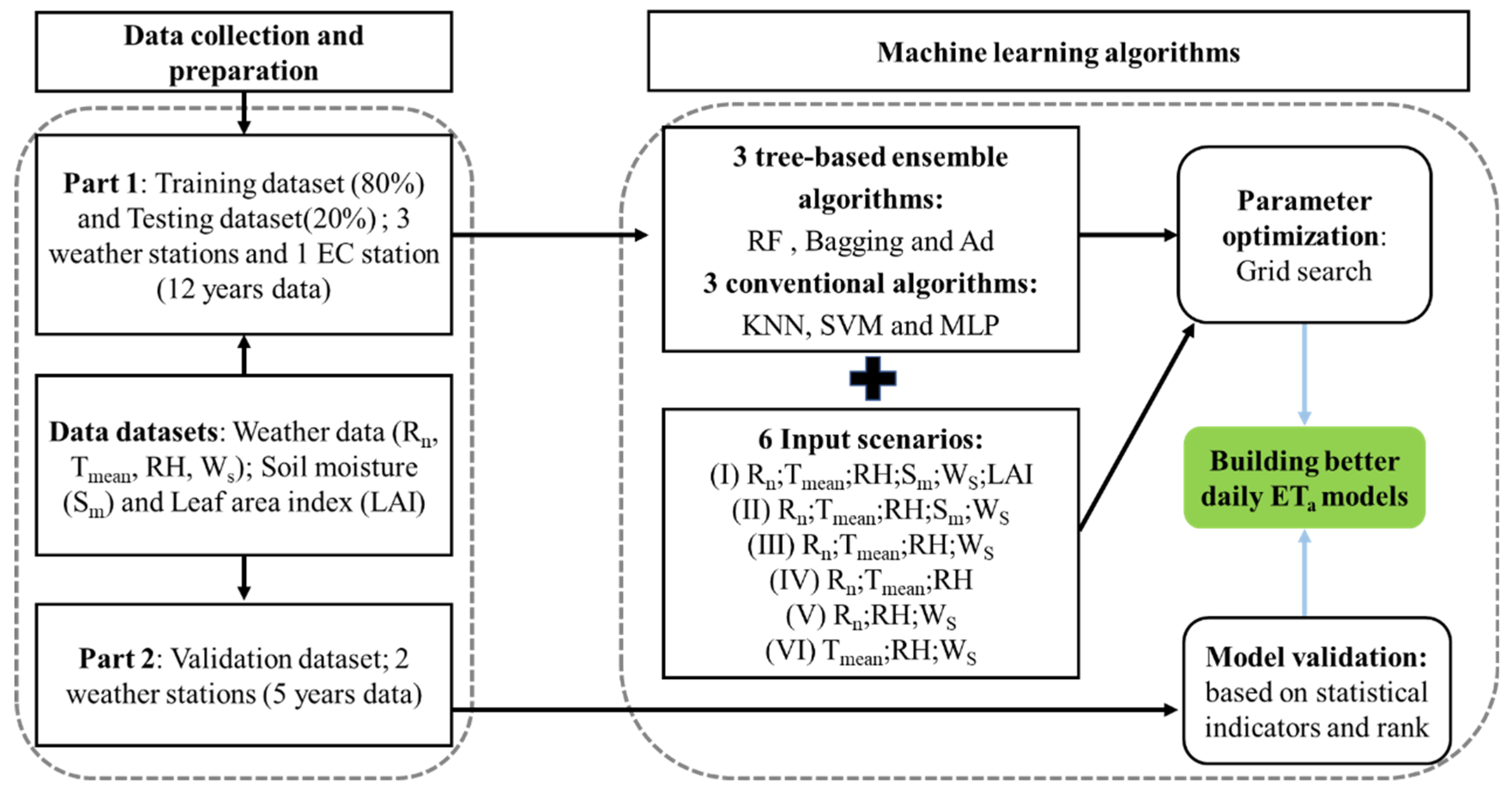
2.2. Data Sources and Meteorological Scenarios

We established five weather stations in our study area, basing them on five tea plantations for meteorological and hydrological observations from 2010 to 2021 (Figure 1c). Meanwhile, an eddy–covariance flux was launched in 2014 (Figure 1c), and it obtained high-frequency energy, water, and carbon fluxes in the tea plantations. For the weather stations, ET_a was calculated using water balance methods during days without rain for 3 consecutive days. For the flux station, ET_a was obtained from the direct measurement of the energy flux. The details of flux data processing can be found in [6]. A brief description of our weather and flux stations is provided in Table 1.

Table 2. Correlation matrix between daily tea plantation ET_a and meteorological data (R_n, T_mean, W_s, RH, and S_m).

	Rn	Tmean	Ws	RH	Sm	ETa
Rn	1
Tmean	0.65	1
Ws	0.08	−0.06	1
RH	−0.37	0.13	−0.29	1
Sm	−0.13	−0.35	−0.04	0.06	1
ETa	0.83	0.71	0.18	−0.17	−0.22	1

presents the correlation matrix of tea plantation ET_a with soil water, vegetation parameters, and meteorological data input variables. The purpose of these correlations was to determine the parameters that could provide the best estimation of overall tea plantation ET_a. The results showed that the relationship between net radiation (R_n) and ET_a (0.83) is higher than the relationship with other variables; that is, R_n exerts the greatest effect on ET_a among the input parameters. The second highest correlation, 0.71, was obtained between mean air temperature (T_mean) and ET_a. Previous studies have also reported that radiation conditions exhibit higher relevance with ET_a in humid regions where water is relatively sufficient [34,35]. Soil moisture (S_m) and mean relative humidity (RH) were negatively correlated with ET_a (values: −0.22 and −0.17, respectively). Meanwhile, the vegetation parameter leaf area index (LAI) was also considered in the ET_a estimation. Accordingly, the parameters were classified by adding the next closest correlation. Six scenarios of meteorological, soil, and vegetation parameters were analyzed using different machine learning algorithms (

Table 3. The input scenarios of variables for different machine learning models.

Scenario	Input Data
	Rn	Tmean	Ws	RH	LAI	Sm
Scenario 1	√	√	√	√	√	√
Scenario 2	√	√	√	√		√
Scenario 3	√	√	√	√
Scenario 4	√	√		√
Scenario 5	√		√	√
Scenario 6		√	√	√

).

2.3. Machine Learning Methods

Given their flexibility and reliability in data pattern recognition, machine learning techniques have elicited considerable attention in various fields [36,37,38]. In recent years, this has included automated machine learning [39], biological process modeling [40], smart city planning [41], and precision agriculture [42]. Various machine learning methods, which have been proven to be effective tools in data mining tasks, exist in the literature. To provide an efficient tea plantation ET_a evaluation model, six widely used machine learning methods, namely, KNN, SVM, RF, MLP, Ada, and bagging, were applied to the estimation of the tea plantations’ ET_a in the current study. The data processing and model building of this study are shown in Figure 2. The machine learning algorithms are briefly described in the succeeding subsections.

2.3.1. K-Nearest Neighbor (KNN)

The KNN algorithm is a common classification method in data mining and statistics. Given its simplicity and outstanding classification performance [43], this model has drawn wide attention from various fields, such as in hydrological modeling [44] and remote-sensing image classification [45]. KNN is nonparametric because it does not assume data distribution [46,47], making the model easy to build in our study. In KNN, the Euclidean distance between the test sample and all the training samples is frequently used to obtain the nearest neighbors of the test data. In accordance with the distance calculation result, the labels of the test samples can be assigned using the majority rule on the basis of the labels of the selected nearest neighbors. K = 5 is proven to be the optimal value in the current study for all the considered models.

2.3.2. Support Vector Machine (SVM)

The SVM algorithm is normally introduced as a supervised learning model, and it has been widely used to deal with classification and regression problems [48,49]. It has also been utilized for prediction [50]. In general, the SVM model aims to generate the best separation hyperplane that can linearly divide classes (Figure S2a) [51]. This modeling process contains the definition of a certain linear function that works to determine a decision boundary for the highest margin, which is illustrated as $2/‖\omega ‖$ in Figure S2a. However, certain minor noisy data must be accepted (Figure S2b) because disregarding them can oversimplify the modeling process and induce limited influence on model performance. The current study adopted SVM to estimate ET_a because of its high efficiency and reliable output. Further details regarding SVM can be found in the literature [52]. The commonly used radial basis function, a nonlinear kernel function, was adopted in this study because it exhibits better performance in evapotranspiration estimation than other kernel functions [53].

2.3.3. Random Forest (RF)

RF is a tree-based supervised EL model for addressing prediction and regression problems [54]; it has been verified as valid in the field of regional evapotranspiration evaluation. This model commonly builds an ensemble of decision trees by using a nonparametric algorithm. Each tree is determined by randomly selecting training samples from the whole feature set. Training normally reserves all the selected features without pruning. Then, the final predictions are obtained by averaging the model output. Considering the independence of trained trees in this model, RF seldom falls into an overfitting problem, indicating that this model is easy to train for practical implementations [55]. In the current study, the number of elements of a leaf node was 5 and the random forests used consisted of 500 trees.

2.3.4. Multilayer Perceptron (MLP)

MLP is a feedforward ANN that is the basis for the development of various deep learning techniques. The classic MLP model generally uses input, hidden, and output layers to deal with complicated classification problems (Figure S3). This model is also efficient in learning a nonlinear function to perform a regression operation. Adjacent layers are fully connected to extract and combine nonlinear features. In particular, the input and hidden layers commonly transform the extracted feature by using a weighted linear algorithm, such as the rectified linear unit function; then, high-level features can be obtained via feature combination [56]. The output layer receives the output from the last hidden layer and converts it into a labeled probability for each category. The neural networks used in the current study have three hidden layers containing hidden neurons. Each hidden layer has four hidden neurons. The number of iterations executed during the training period of the backpropagation algorithm is 600. The learning rate and momentum rate of the backpropagation algorithm are 0.3 and 0.2, respectively.

2.3.5. Adaptive Boosting (AdaBoost)

The AdaBoost model is known as a successful and reliable artificial intelligence method in the field of classification, prediction, and recognition due to its advantage of adaptive augmentation [9,57,58]. In general, the working principle of this method includes the following: (I) randomly selecting training subsets at the beginning; (II) repeating the training model by selecting a training set based on an accurate estimate of the last training session; and (III) assigning higher weights to erroneous categorical observations, so that the misclassified sample data receive attention in the next iteration of training [59]. The final robust classifier that combines several weak classifiers can accurately predict the class of new observations. A decision tree was boosted in the current study, and the number of estimators was fixed to 30 to ensure the best results. Meanwhile, the number of learning rates was fixed to 1.

2.3.6. Bagging

Bagging is a machine learning ensemble meta-algorithm for improving forecast accuracy by using multiple versions of a predictor to generate an aggregated predictor [60,61]. This model created sample sets by randomly training sample sets and then used the obtained subsets to train basic algorithms for combination. Consequently, final accuracy can be improved using the output results from multiple models [62]. The training of basic algorithms in bagging is performed in parallel; as a result, this condition can highly promote training efficiency. Compared with the other models, bagging performs well in mitigating the overfitting problem. The classification and regression tree was selected as the base estimator in the current study. The numbers of estimators and learning rates were 50 and 1, respectively.

In this study, 80% of the data from three weather stations (SSY, TMHS, and HB) and the flux station for tea plantations (tea plantation flux site) were used for training, while the remaining 20% of the data were used for testing. The data from the PQ and TMXM stations were used for validation. The described algorithms were implemented in a specific Python code.

2.4. Performance Comparison Criteria

The performance of all models was evaluated using the mean absolute error (MAE), root-mean-square error (RMSE), Nash–Sutcliffe efficiency coefficient (NSE), coefficient of determination (R²), and slope between measured and simulated ET_a values, in accordance with the equations below. Meanwhile, the experimental model of actual evapotranspiration (“GG”) was also used to compare with these machine learning models. The details of the GG model are described in the Supplementary Materials.

$$\mathrm{M}\mathrm{A}\mathrm{E}=\left|\frac{{\sum }_{\mathrm{i}=1}^{\mathrm{n}}\left({\mathrm{P}}_{\mathrm{i}}-{\mathrm{O}}_{\mathrm{i}}\right)}{\mathrm{n}}\right|$$

where n is the total number of observed data; ${\mathrm{P}}_{\mathrm{i}}$ is the predictive value of tea plantation evapotranspiration; and ${\mathrm{O}}_{\mathrm{i}}$ is the observed value.

$$\mathrm{R}\mathrm{M}\mathrm{S}\mathrm{E}=\sqrt{\frac{{\sum }_{\mathrm{i}=1}^{\mathrm{n}}{\left({\mathrm{P}}_{\mathrm{i}}-{\mathrm{O}}_{\mathrm{i}}\right)}^2}{\mathrm{n}}}$$

$${\mathrm{R}}^2=\frac{{\sum }_{\mathrm{i}=1}^{\mathrm{n}}{\left({\mathrm{P}}_{\mathrm{i}}-{\mathrm{O}}_{\mathrm{i}}\right)}^2}{{\sum }_{\mathrm{i}=1}^{\mathrm{n}}{\left({\mathrm{O}}_{\mathrm{m}}-{\mathrm{O}}_{\mathrm{i}}\right)}^2}$$

where ${\mathrm{O}}_{\mathrm{m}}$ is the mean of the observed values of tea plantation evapotranspiration.

MAE and RMSE with smaller values and R² with higher values confirm better model performance.

3. Results and Discussion

3.1. Climate and Evapotranspiration Characteristics

Daily average R_n, T_mean, RH, W_s (at 2 m height), and ET_a across the observation stations for the tea plantations were 7.31 MJ m⁻² day⁻¹, 16.59 °C, 78%, 1.31 m s⁻¹, and 2.05 mm day⁻¹, respectively, during the study period. The average monthly distributions of R_n, T_mean, RH, W_s, and ET_a are presented in Figure 3. Similar seasonal patterns were observed for R_n, T_mean, and ET_a. Low values of R_n, T_mean, and ET_a were recorded in January and December, whereas higher values generally occurred in July and August (Figure 3). The maximum R_n, T_mean, and ET_a reached 18.93 MJ m⁻² day⁻¹, 34.05 °C, and 6.9 mm day⁻¹, respectively, in July during the study period. About 65–75% RH was observed in February, April, and October, whereas a high RH of more than 75% was reported in other months. Low W_s (0.88–1.05 m s⁻¹) were experienced in July, September, and October. By contrast, May, April, and August presented higher W_s (1.5–1.9 m s⁻¹) (Figure 3c).

3.2. Performance of Machine Learning Models

Table 4. Model comparison–summary of the results in the testing phase.

Algorithm	Model	Scenario	MAE	RMSE	NSE	Slope	R2
			(mm day−1)	(mm day−1)
K-Nearest Neighbor	kNN6	Scenario 1	0.3630	0.4910	0.872	0.841	0.872
	kNN5	Scenario 2	0.3799	0.5216	0.766	0.824	0.856
	kNN4	Scenario 3	0.3756	0.5192	0.857	0.839	0.857
	kNN3a	Scenario 4	0.3843	0.5213	0.856	0.836	0.856
	kNN3b	Scenario 5	0.4486	0.6008	0.808	0.786	0.808
	kNN3c	Scenario 6	0.5709	0.7799	0.677	0.682	0.671
Support Vector Machine	SVM6	Scenario 1	0.3213	0.4602	0.887	0.871	0.887
	SVM5	Scenario 2	0.3360	0.4772	0.804	0.845	0.879
	SVM4	Scenario 3	0.3483	0.4902	0.873	0.872	0.873
	SVM3a	Scenario 4	0.3581	0.5223	0.855	0.829	0.855
	SVM3b	Scenario 5	0.3885	0.5403	0.845	0.816	0.845
	SVM3c	Scenario 6	0.5333	0.7407	0.709	0.694	0.710
Multilayer Perceptron	MLP6	Scenario 1	0.3630	0.5616	0.837	0.745	0.833
	MLP5	Scenario 2	0.4181	0.5812	0.704	0.716	0.819
	MLP4	Scenario 3	0.4095	0.5680	0.815	0.724	0.828
	MLP3a	Scenario 4	0.4191	0.5809	0.823	0.729	0.821
	MLP3b	Scenario 5	0.4728	0.6246	0.791	0.677	0.793
	MLP3c	Scenario 6	0.6330	0.8590	0.609	0.517	0.610
Adaptive boosting	AdaBoost6	Scenario 1	0.4072	0.5197	0.854	0.772	0.849
	AdaBoost5	Scenario 2	0.3936	0.5292	0.846	0.762	0.851
	AdaBoost4	Scenario 3	0.4122	0.5452	0.848	0.761	0.842
	AdaBoost3a	Scenario 4	0.4157	0.5564	0.831	0.753	0.835
	AdaBoost3b	Scenario 5	0.4805	0.6241	0.803	0.735	0.793
	AdaBoost3c	Scenario 6	0.5991	0.7734	0.682	0.606	0.683
Bagging	Bg6	Scenario 1	0.3275	0.4368	0.887	0.869	0.893
	Bg5	Scenario 2	0.3514	0.4778	0.870	0.842	0.878
	Bg4	Scenario 3	0.3638	0.4841	0.871	0.836	0.876
	Bg3a	Scenario 4	0.3872	0.5158	0.858	0.843	0.842
	Bg3b	Scenario 5	0.4238	0.5593	0.818	0.813	0.833
	Bg3c	Scenario 6	0.5676	0.7720	0.694	0.703	0.684
Random Forest	RF6	Scenario 1	0.3186	0.4102	0.897	0.870	0.906
	RF5	Scenario 2	0.3407	0.4645	0.815	0.856	0.886
	RF4	Scenario 3	0.3504	0.4717	0.877	0.851	0.882
	RF3a	Scenario 4	0.3758	0.5138	0.861	0.841	0.860
	RF3b	Scenario 5	0.4170	0.5570	0.836	0.810	0.835
	RF3c	Scenario 6	0.5441	0.7319	0.713	0.705	0.710
GG model		[63]	0.3412	0.4900	0.837	0.846	0.870

provides the performance of three EL machine learning models (RF, bagging, and Ad) and the three common machine learning models (KNN, SVM, and MLP) in predicting daily tea plantation ET_a during the testing phase under six input scenarios. The statistical results indicated that the RF model had higher R² values (0.84–0.91) and lower RMSE (0.41–0.56 mm day⁻¹) during the testing phase, followed by bagging, SVM, KNN, and Ad, except in Scenario 6, whereas MLP exhibited the lowest performance among the 36 estimation models in predicting tea plantation ET_a (Table 4). In addition, the experimental model of evapotranspiration (the “GG” model) has good simulation results for tea plantation evapotranspiration (R²: 0.87; RMSE: 0.49 mm day⁻¹). However, the experimental model needed more driving data (for example, the soil heat flux and drying force) than that required for the machine learning models, which are hard to obtain from conventional meteorological stations. Moreover, there are different performances for the estimation of tea plantations’ evapotranspiration between the six datasets’ scenarios. In Scenario 1, all the models achieved high-performance accuracy with high values of R² (0.833–0.906) and low RMSE (0.4102–0.5616 mm day⁻¹). The datasets for Scenarios 2, 3, 4, and 5 provided the second, third, fourth, and fifth performance accuracy, respectively. However, for Scenario 6, performance accuracy dropped dramatically in all the models, with high RMSE and MAE but low R². ET_a values in the validation phase illustrate that the machine learning models exhibit varying prediction accuracy under different input scenarios (Figure 4). A similar pattern was observed in the testing phase. RF also achieved the best performance in the validation phase for assessing the daily ET_a of tea plantations by using different input combination strategies, followed by bagging and SVM. In general, EL models (RF and bagging) were superior to the other models (KNN, MLP, Ad, and SVM). The authors of [48] revealed that RF outperformed other models in evaluating the ET_a of humid subtropical wetlands. In [18], it was found that tree-based EL models obtained more precise estimation values of evapotranspiration than common machine learning models (e.g., SVM). Meanwhile, slight differences were observed between the bagging and RF models in estimating tea plantations’ ET_a (MAE < 3% and RMSE < 2.8%) for the six input scenarios (Table 4). The results also supported our hypothesis that bagging achieved high prediction accuracy in daily ET_a because its algorithm principles were similar to those of RF. By contrast, the performance of the Ad model did not meet its expectations. Overall, the RF, bagging, and SVM models were the best models for estimating the daily ET_a of tea plantations on the basis of the aforementioned performance comparison criteria.

Different variable scenarios also play a crucial part in the estimation precision of machine learning models for tea plantation ET_a. In the validation phase (Figure 4), the models that used the complete climate and plant data scenario (Scenario 1: six-variable models) exhibited the best prediction accuracy compared with the incomplete input data scenarios (Scenarios 2 to 6) (Figure 4). However, in Scenario 6 (T_mean; mean RH; W_S, 3c-variable models), all the models presented the worst performance (Figure 4f). Previous studies have also documented that machine learning models with temperature and radiation variables (e.g., sunshine duration and R_n) can obtain reasonable evapotranspiration estimation accuracy in a humid region [64]. Our results indicated that R_n was considerably more significant than T_mean and mean RH for daily tea plantation ET_a, and the models based on R_n could generally generate satisfactory ET_a estimates for tea plantations. Such a finding is also consistent with earlier studies [6,65], wherein radiation conditions are essential variables for ET_a estimation in humid climatic regions due to the energy limit for crop evapotranspiration. Notably, all machine learning models exhibit a tendency to underestimate ET_a for tea plantations with ET_a > 6 mm day⁻¹. This uncertainty is discussed further in the next section.

As an effective tool, Taylor diagrams were used to elicit a comparison between the considered machine learning models under six input scenarios for tea plantation ET_a (Figure 5). Figure 5 provides a summary of the models in terms of statistical parameters with the observed data [66,67]. The results also supported that the RF, bagging, and SVM models were the best for estimating daily tea plantation ET_a.

3.3. Stability Appraisal and Uncertainty of Machine Learning Models

Figure 6 shows the average RMSE of all machine learning algorithms in our study during the validation and testing phases under six input scenarios. The results show that RF and bagging models exhibited improved steadiness with low RMSE values increasing in the validation phase over the testing phase. By contrast, MLP was the worst-performing model compared with the Ad, KNN, SVM, bagging, and RF models. The RF and bagging models reliably demonstrated the lowest percentage increase (−15.3% to +18.5%) in validation-phase RMSE over testing phase RMSE among the six machine learning algorithms, suggesting that the RF and bagging models would considerably improve the prediction accuracy when using new climate datasets with high stability. Our results are consistent with the outcomes of [32]. They also reported that the RF model presented a lower increase in testing RMSE from 0 to 49% in the validation phase over the testing phase. The authors of [68] revealed that RF exhibited high performance in evapotranspiration estimation by using the FLUXNET2015 dataset. However, the results of our study disagreed with those of [69], who reported that the RMSE increase rate for the bagging model in the test phase was typically higher than the rates for other machine learning models. Moreover, EL algorithms, including bagging, RF, and Ad, exhibited inferior performance in regression problems due to the impaired ability to provide a constant output [69]. In our study, however, the RF and bagging models displayed good stability with a satisfactory percentage increase, wherein the decision tree might provide more weight for points that were not predicted using the previous predictor and finally reserved the weighted voting right to overcome the estimation difficulty of overfitting [70]. However, the ensemble model Ad could not produce good prediction accuracy in our case. In particular, in the 6–8 mm day⁻¹ range (early-growing and mid-growing seasons), it had a higher RMSE than the RF and bagging models (Figure 7 and Figure 8). This result was largely due to the high sensitivity to “abnormal samples” of Ad during that period (high plant physiology limits), which obtained a high weight in iteration, affecting the prediction accuracy of the final strong learner. This phenomenon was also documented by many researchers who used the Ad model to resolve regression problems in hydrology and agriculture studies [71,72].

The levels of accuracy in different estimation ranges and seasons of daily tea plantation ET_a were assessed (Figure 7 and Figure 8). The range of daily ET_a observed values in the validation phase was divided into four sub-intervals: 0–2, 2–4, 4–6, and 6–8 mm day⁻¹. Meanwhile, the performance of different seasons, i.e., the early-growing season (E), mid-growing season (M), late-growing season (L), and non-growing season (N) with different estimation ranges of ET_a, were also investigated. All models presented the highest RMSE values in the sub-interval of 6–8 mm day⁻¹ (Figure 7). Except for the RF and bagging models, RMSE was always above 1.0 mm day⁻¹ for the other models in the sub-interval under all the scenarios. It even exceeded 1.5 mm day⁻¹ for the MLP model. In Scenarios 5 and 6, RMSE values even exceeded 2.0 mm day⁻¹ for the MLP model (Figure 7e,f). By contrast, in the sub-intervals of 0–2 mm day⁻¹ and 2–4 mm day⁻¹, all the models had a higher prediction accuracy (RMSE < 0.6 mm day⁻¹, except for Scenario 6, Figure 7f). In general, the RF and bagging models exhibited the highest stability with a lower RMSE increase (RMSE < 0.32–0.81 mm day⁻¹) than the other models at all sub-intervals. At the seasonal scale, except for the RF and bagging models, the other models also had higher RMSE (0.5–1.2 mm day⁻¹) in the early-growing and mid-growing seasons, which increased from 31% to 137% relative to the RF and bagging models. In other seasons, except for Scenario 6, the RMSE of all the models was within 0.5 mm day⁻¹. Meanwhile, the differences in RMSE values between the RF and bagging models were within 10%. These results also suggest that the tree-based EL (RF and bagging algorithms) exhibit good potential for tea plantation ET_a estimation with a higher stability.

However, the results also indicate high uncertainty for estimating daily tea plantation ET_a in the sub-interval of 6–8 mm day⁻¹ (Figure 7 and Figure 8) largely due to the significant underestimation of ET_a by machine learning models (Figure 4). Many similar results for the underestimation of ET_a in high-value areas have been reported using machine learning in humid region ecosystems [32,48,68]. Notably, daily tea plantation ET_a in the sub-interval of 6–8 mm day⁻¹ is concentrated in the early- and mid-growing seasons. In our study site, energy conditions are the key control factors of daily tea plantation ET_a. However, during the early-growing and mid-growing seasons, the plant physiology limit for ET_a increased due to high temperatures and heat stress. Our observation results in the tea plantation flux site also captured the physiology limit for ET_a, where canopy conductance decreased, limiting water loss and promoting water use efficiency (WUE) with high heat stress during the two seasons [6,73]. These results revealed that physiological responses to high temperatures and heat stress would reduce ET_a, even if R_n was high. However, as discussed above, a significant positive correlation relationship existed between R_n and ET_a for tea plantations (Table 2), which is the basis for the daily tea plantation ET_a estimation by our machine learning models. However, physiological limits might lead to low ET_a under high R_n conditions with high temperatures and heat stress. In addition, the extreme climate events and human disturbance altered the stationary process of meteorological and vegetation ecological data, which might lead to higher RMSE values for predicting tea plantation ET_a in the two seasons. Hence, we speculated that the underestimation of ET_a for our models was primarily due to the physiological limitations of tea plantations and the nonstationary nature of the data during the early-growing and mid-growing seasons.

3.4. Contribution of Influencing Factors to the Predicted Daily ET_a of Tea Plantation

The contributions of the influencing factors on the predicted daily ET_a from the studied models were assessed using the Shapley value. Figure 9 displays the key statistical parameters for the six machine learning models by using the whole dataset (Scenario 1) in the validation phase. All models consistently detected R_n as the most vital factor. Meanwhile, a positive correlation relationship between daily ET_a and R_n was also found. In addition, T_mean also made a high contribution to tea plantation ET_a estimation for all machine learning models. By contrast, the contributions of other features varied in the different models. In the KNN and SVM models, W_s was the third important feature, and the effects of the remaining features were considerably smaller. For MLP and RF models, LAI was the third important feature. Meanwhile, RH was the third important feature for the Ad and bagging models. However, the importance of LAI and RH also decreased significantly. The contribution of S_m was considerably less of a feature for all models in our study. The results suggested that energy conditions (R_n and T_mean) are the key drivers for tea plantation ET_a estimation. This finding agreed with those of previous studies, which reported that solar radiation and temperature are the most important climatic variables that influence ET_a variation in different ecosystems in humid regions [6,68]. Meanwhile, this finding was further supported by observation studies that used eddy covariance, which implied that R_n acted as a primary driver of evapotranspiration in tea plantations and determined the temporal variation in ET_a by more than 70% for tea plantations in our study area [5,6]. These results also suggest that the models that used machine learning methods in our study possess a certain physical mechanism for the ET_a estimation of tea plantations.

Apart from the strong effect of energy conditions on tea plantation ET_a estimation, intense extreme climatic events and human-induced activities, such as canopy pruning, weeding, drainage, and extreme drought, will alter the water and heat exchange process, thereby increasing the complexity of the evaluation process of tea plantation ET_a. Significant underestimation of ET_a by our machine learning models was noted with extreme climatic events and human-induced events in the current study. Hence, the contributions of global warming and human activities to the change in ET_a should be noted in the future and the prediction accuracy of evapotranspiration using machine learning methods should be improved to provide better decision making for the sustainable water resources and agricultural irrigation system planning of tea plantations.

4. Conclusions

In this study, we presented the potential of EL models (RF, bagging, and Ada) for precisely estimating the daily ET_a of tea plantations with six scenarios of available tea plantation meteorological and evapotranspiration data collected over 12 years (2010–2021). The results suggest that the RF model exhibited superior performance, with higher values of R² (0.84–0.91) and lower values of MAE (0.32–0.42 mm day⁻¹) and RMSE (0.41–0.56 mm day⁻¹) compared with the other state-of-the-art models for predicting the daily ET_a of tea plantations. Meanwhile, RF and bagging models exhibited the highest steadiness with low RMSE values increasing (−15.3~+18.5%) in the validation phase over the testing phase. Considering the high prediction accuracy and dependability of the studied models, the RF and bagging models can be recommended for the daily ET_a estimation of tea plantations. The importance analysis from the studied models determined that R_n and T_mean are the most critical influential variables that affect the daily dynamics of the observed and predicted ET_a values for tea plantations. In the absence of climatic datasets, R_n, T_mean, and RH combinations (Scenario 4) achieved reasonable precision in assessing the daily ET_a of tea plantations in all the models. The results of this study will contribute to the management of water resources for tea plantations.

References

1. FAO. FAO Stat Data. 2017. Available online: http://faostat.fao.org (accessed on 27 December 2017).
2. NBSC. China Statistical Yearbook, Annual Publication; National Bureau of Statistics of China: Beijing, China, 2017. Available online: http://www.stats.gov.cn/tjsj/ndsj/2017/indexch.htm (accessed on 1 July 2018).
3. Chiu, Y.C.; Chen, B.J.; Su, Y.S.; Huang, W.D.; Chen, C.C. A Leaf Disc Assay for Evaluating the Response of Tea (Camellia sinensis) to PEG-Induced Osmotic Stress and Protective Effects of Azoxystrobin against Drought. Plants 2021, 10, 546. [Google Scholar] [CrossRef] [PubMed]
4. Zhang, X.C.; Wu, H.H.; Chen, J.G.; Chen, L.M.; Chang, N.; Ge, G.F.; Wan, X. Higher ROS scavenging ability and plasma membrane H+-ATPase activity are associated with potassium retention in drought tolerant tea plants. J. Plant Nutr. Soil Sci. 2020, 183, 406–415. [Google Scholar] [CrossRef]
5. Geng, J.W.; Li, H.P.; Pang, J.P.; Zhang, W.S.; Shi, Y.J. The effects of land-use conversion on evapotranspiration and water balance of subtropical forest and managed tea plantation in Taihu Lake Basin, China. Hydrol. Process. 2022, 36, e14652. [Google Scholar] [CrossRef]
6. Geng, J.; Li, H.; Pang, J.; Zhang, W.; Chen, D. Dynamics and environmental controls of energy exchange and evapotranspiration in a hilly tea plantation, China. Agric. Water Manag. 2020, 241, 106364. [Google Scholar] [CrossRef]
7. Zheng, S.H.; Ni, K.; Ji, L.F.; Zhao, C.G.; Chai, H.L.; Yi, X.Y.; He, W.; Ruan, J. Estimation of Evapotranspiration and Crop Coefficient of Rain-Fed Tea Plants under a Subtropical Climate. Agronomy 2021, 11, 2332. [Google Scholar] [CrossRef]
8. Liu, B.H.; Xu, M.; Henderson, M.; Qi, Y. Observed trends of precipitation amount, frequency, and intensity in China, 1960–2000. J. Geophys. Res. Atmos. 2005, 110, D8. [Google Scholar] [CrossRef]
9. Liu, H.; Tian, H.-Q.; Li, Y.-F.; Zhang, L. Comparison of four Adaboost algorithm based artificial neural networks in wind speed predictions. Energy Convers. Manag. 2015, 92, 67–81. [Google Scholar] [CrossRef]
10. Ma, S.M.; Zhou, T.J.; Dai, A.G.; Han, Z.Y. Observed Changes in the Distributions of Daily Precipitation Frequency and Amount over China from 1960 to 2013. J. Clim. 2015, 28, 6960–6978. [Google Scholar] [CrossRef]
11. Kirkham, R.R.; Gee, G.W.; Jones, T.L. Weighing lysimeters for long-term water-balance investigations at remote sites. Soil Sci. Soc. Am. J. 1984, 48, 1203–1205. [Google Scholar] [CrossRef]
12. Qiu, J.; Chen, H.; Wang, P.; Liu, Y.; Xia, X. Recent progress in atmospheric observation research in China. Adv. Atmos. Sci. 2007, 24, 940–953. [Google Scholar] [CrossRef]
13. Varmaghani, A.; Eichinger, W.E.; Prueger, J.H. Modification of FAO Penman-Monteith equation for minor components of energy. Hydrol. Res. 2019, 50, 607–615. [Google Scholar] [CrossRef]
14. Xiao, J.; Sun, G.; Chen, J.; Chen, H.; Chen, S.; Dong, G.; Gao, S.; Guo, H.; Guo, J.; Han, S.; et al. Carbon fluxes, evapotranspiration, and water use efficiency of terrestrial ecosystems in China. Agric. For. Meteorol. 2013, 182, 76–90. [Google Scholar] [CrossRef]
15. Corbari, C.; Paleari, R.; Mantovani, F.; Tarro, S.; Mancini, M. A weighting lysimeter for a laboratory experiment on water and energy fluxes measurements and hydrological models verification. In EGU General Assembly Conference Abstracts; EGU: Vienna, Austria, 2017. [Google Scholar]
16. Irmak, S. Nebraska water and energy flux measurement, modeling, and research network (NEBFLUX). Trans. ASABE 2010, 53, 1097–1115. [Google Scholar] [CrossRef]
17. Hu, S.; Zhao, C.; Li, J.; Wang, F.; Chen, Y. Discussion and reassessment of the method used for accepting or rejecting data observed by a Bowen ratio system. Hydrol. Process. 2014, 28, 4506–4510. [Google Scholar] [CrossRef]
18. Huang, G.; Wu, L.; Ma, X.; Zhang, W.; Fan, J.; Yu, X.; Zeng, W.; Zhou, H. Evaluation of CatBoost method for prediction of reference evapotranspiration in humid regions. J. Hydrol. 2019, 574, 1029–1041. [Google Scholar] [CrossRef]
19. Huang, M.F.; Liu, S.M.; Guo, X.Y.; Zhu, Q.J.; Li, J.T. Analysis of the factors influencing surface sensible heat fluxes with large aperture scintillometers. In Proceedings of the IGARSS 2004: IEEE International Geoscience and Remote Sensing Symposium, Anchorage, AK, USA, 20–24 September 2004; pp. 4281–4284. [Google Scholar]
20. Li, Z.Q.; Yu, G.R.; Wen, X.F.; Zhang, L.M.; Ren, C.Y.; Fu, Y.L. Energy balance closure at ChinaFLUX sites. Sci. China Ser. D Earth Sci. 2005, 48, 51–62. [Google Scholar]
21. Wilson, K.; Goldstein, A.; Falge, E.; Aubinet, M.; Baldocchi, D.; Berbigier, P.; Bernhofer, C.; Ceulemans, R.; Dolman, H.; Field, C.; et al. Energy balance closure at FLUXNET sites. Agric. For. Meteorol. 2002, 113, 223–243. [Google Scholar] [CrossRef]
22. Gelybo, G.; Barcza, Z.; Kern, A.; Kljun, N. Effect of spatial heterogeneity on the validation of remote sensing based GPP estimations. Agric. For. Meteorol. 2013, 174, 43–53. [Google Scholar] [CrossRef]
23. Farahani, H.J.; Howell, T.A.; Shuttleworth, W.J.; Bausch, W.C. Evapotranspiration: Progress in measurement and modeling in agriculture. Trans. ASABE 2007, 50, 1627–1638. [Google Scholar] [CrossRef]
24. Howell, T. Enhanceing water use efficiency in irrigated agriculture. Agron. J. 2001, 93, 281–289. [Google Scholar] [CrossRef]
25. Lecina, S.; Martínez-Cob, A.; Pérez, P.J.; Villalobos, F.J.; Baselga, J.J. Fixed versus variable bulk canopy resistance for reference evapotranspiration estimation using the Penman–Monteith equation under semiarid conditions. Agric. Water Manag. 2003, 60, 181–198. [Google Scholar] [CrossRef]
26. Tang, D.; Feng, Y.; Gong, D.; Hao, W.; Cui, N. Evaluation of artificial intelligence models for actual crop evapotranspiration modeling in mulched and non-mulched maize croplands. Comput. Electron. Agric. 2018, 152, 375–384. [Google Scholar] [CrossRef]
27. Azzam, A.; Zhang, W.; Akhtar, F.; Shaheen, Z.; Elbeltagi, A. Estimation of green and blue water evapotranspiration using machine learning algorithms with limited meteorological data: A case study in Amu Darya River Basin, Central Asia. Comput. Electron. Agric. 2022, 202, 107403. [Google Scholar] [CrossRef]
28. Dou, X.; Yang, Y. Evapotranspiration estimation using four different machine learning approaches in different terrestrial ecosystems. Comput. Electron. Agric. 2018, 148, 95–106. [Google Scholar] [CrossRef]
29. Zhang, C.; Brodylo, D.; Rahman, M.; Rahman, M.A.; Douglas, T.A.; Comas, X. Using an object-based machine learning ensemble approach to upscale evapotranspiration measured from eddy covariance towers in a subtropical wetland. Sci. Total Environ. 2022, 831, 154969. [Google Scholar] [CrossRef] [PubMed]
30. Fan, J.; Yue, W.; Wu, L.; Zhang, F.; Cai, H.; Wang, X.; Lu, X.; Xiang, Y. Evaluation of SVM, ELM and four tree-based ensemble models for predicting daily reference evapotranspiration using limited meteorological data in different climates of China. Agric. For. Meteorol. 2018, 263, 225–241. [Google Scholar] [CrossRef]
31. Gonzalo-Martin, C.; Lillo-Saavedra, M.; Garcia-Pedrero, A.; Lagos, O.; Menasalvas, E. Daily Evapotranspiration Mapping Using Regression Random Forest Models. IEEE J. Sel. Top. Appl. Earth Obs. Remote Sens. 2017, 10, 5359–5368. [Google Scholar] [CrossRef]
32. Salam, R.; Islam, A.R.M.T. Potential of RT, bagging and RS ensemble learning algorithms for reference evapotranspiration prediction using climatic data-limited humid region in Bangladesh. J. Hydrol. 2020, 590, 125241. [Google Scholar] [CrossRef]
33. Shao, G.; Han, W.; Zhang, H.; Liu, S.; Wang, Y.; Zhang, L.; Cui, X. Mapping maize crop coefficient Kc using random forest algorithm based on leaf area index and UAV-based multispectral vegetation indices. Agric. Water Manag. 2021, 252, 106906. [Google Scholar] [CrossRef]
34. Wang, Y.; Zou, Y.; Cai, H.; Zeng, Y.; He, J.; Yu, L.; Zhang, C.; Saddique, Q.; Peng, X.; Siddique, K.H.; et al. Seasonal variation and controlling factors of evapotranspiration over dry semi-humid cropland in Guanzhong Plain, China. Agric. Water Manag. 2022, 259, 107242. [Google Scholar] [CrossRef]
35. Zhang, H.; Hu, Y.; Cai, J.; Li, X.; Tian, B.; Zhang, Q.; An, W. Calculation of evapotranspiration in different climatic zones combining the long-term monitoring data with bootstrap method. Environ. Res. 2020, 191, 110200. [Google Scholar] [CrossRef] [PubMed]
36. Lood, C.; Boeckaerts, D.; Stock, M.; De Baets, B.; Lavigne, R.; van Noort, V.; Briers, Y. Digital phagograms: Predicting phage infectivity through a multilayer machine learning approach. Curr. Opin. Virol. 2022, 52, 174–181. [Google Scholar] [CrossRef] [PubMed]
37. Rawson, A.; Brito, M.; Sabeur, Z.; Tran-Thanh, L. A machine learning approach for monitoring ship safety in extreme weather events. Saf. Sci. 2021, 141, 105336. [Google Scholar] [CrossRef]
38. Sirsat, M.S.; Fermé, E.; Câmara, J. Machine Learning for Brain Stroke: A Review. J. Stroke Cerebrovasc. Dis. 2020, 29, 105162. [Google Scholar] [CrossRef] [PubMed]
39. Waring, J.; Lindvall, C.; Umeton, R. Automated machine learning: Review of the state-of-the-art and opportunities for healthcare. Artif. Intell. Med. 2020, 104, 101822. [Google Scholar] [CrossRef]
40. Greener, J.G.; Kandathil, S.M.; Moffat, L.; Jones, D.T. A guide to machine learning for biologists. Nat. Rev. Mol. Cell Biol. 2022, 23, 40–55. [Google Scholar] [CrossRef]
41. Khalid, M.; Wang, L.; Wang, K.; Pan, C.; Aslam, N.; Cao, Y. Deep Reinforcement Learning-Based Long-Range Autonomous Valet Parking for Smart Cities. Sustain. Cities Soc. 2021, 89, 104311. [Google Scholar] [CrossRef]
42. Condran, S.; Bewong, M.; Islam, M.Z.; Maphosa, L.; Zheng, L. Machine Learning in Precision Agriculture: A Survey on Trends, Applications and Evaluations Over Two Decades. IEEE Access 2022, 10, 73786–73803. [Google Scholar] [CrossRef]
43. Zhang, S.; Li, X.; Zong, M.; Zhu, X.; Wang, R. Efficient kNN Classification with Different Numbers of Nearest Neighbors. IEEE Trans. Neural Netw. Learn. Syst. 2017, 29, 1774–1785. [Google Scholar] [CrossRef]
44. Shamshirband, S.; Hashemi, S.; Salimi, H.; Samadianfard, S.; Asadi, E.; Shadkani, S.; Kargar, K.; Mosavi, A.; Nabipour, N.; Chau, K.W. Predicting Standardized Streamflow index for hydrological drought using machine learning models. Eng. Appl. Comput. Fluid Mech. 2020, 14, 339–350. [Google Scholar] [CrossRef]
45. Kang, J.; Fernandez-Beltran, R.; Hong, D.; Chanussot, J.; Plaza, A. Graph Relation Network: Modeling Relations Between Scenes for Multilabel Remote-Sensing Image Classification and Retrieval. IEEE Trans. Geosci. Remote Sens. 2021, 59, 4355–4369. [Google Scholar] [CrossRef]
46. Chitralekha, G.; Roogi, J.M. A Quick Review of ML Algorithms. In Proceedings of the 2021 6th International Conference on Communication and Electronics Systems (ICCES), Coimbatre, India, 8–10 July 2021. [Google Scholar]
47. Karmani, P.; Chandio, A.A.; Korejo, I.A.; Chandio, M.S. A Review of Machine Learning for Healthcare Informatics Specifically Tuberculosis Disease Diagnostics. In Proceedings of the Intelligent Technologies and Applications: First International Conference, INTAP 2018, Bahawalpur, Pakistan, 23–25 October 2018; Springer: Berlin/Heidelberg, Germany, 2019; Volume 932, pp. 50–61. [Google Scholar]
48. Granata, F.; Gargano, R.; de Marinis, G. Artificial intelligence based approaches to evaluate actual evapotranspiration in wetlands. Sci. Total Environ. 2020, 703, 135653. [Google Scholar] [CrossRef] [PubMed]
49. Vapnik, V.N. An overview of statistical learning theory. IEEE Trans. Neural Netw. 1999, 10, 988–999. [Google Scholar] [CrossRef] [PubMed]
50. Liao, Y.; Han, L.; Wang, H.; Zhang, H. Prediction Models for Railway Track Geometry Degradation Using Machine Learning Methods: A Review. Sensors 2022, 22, 7275. [Google Scholar] [CrossRef] [PubMed]
51. Bektaş, J. EKSL: An effective novel dynamic ensemble model for unbalanced datasets based on LR and SVM hyperplane-distances. Inf. Sci. 2022, 597, 182–192. [Google Scholar] [CrossRef]
52. Moosaei, H.; Ganaie, M.A.; Hladík, M.; Tanveer, M. Inverse free reduced universum twin support vector machine for imbalanced data classification. Neural Netw. 2022, 157, 125–135. [Google Scholar] [CrossRef]
53. Kisi, O. Pan evaporation modeling using least square support vector machine, multivariate adaptive regression splines and M5 model tree. J. Hydrol. 2015, 528, 312–320. [Google Scholar] [CrossRef]
54. Breiman, L. Random Forests. Mach. Learn. 2001, 45, 5–32. [Google Scholar] [CrossRef]
55. Xu, T.; Guo, Z.; Liu, S.; He, X.; Meng, Y.; Xu, Z.; Xia, Y.; Xiao, J.; Zhang, Y.; Ma, Y.; et al. Evaluating Different Machine Learning Methods for Upscaling Evapotranspiration from Flux Towers to the Regional Scale. J. Geophys. Res. Atmos. 2018, 123, 8674–8690. [Google Scholar] [CrossRef]
56. Deng, K.; Zhao, H.; Li, N.; Wei, W. Identification of minerals in hyperspectral imagery based on the attenuation spectral absorption index vector using a multilayer perceptron. Remote Sens. Lett. 2021, 12, 449–458. [Google Scholar] [CrossRef]
57. Huang, X.; Li, Z.; Jin, Y.; Zhang, W. Fair-AdaBoost: Extending AdaBoost method to achieve fair classification. Expert Syst. Appl. 2022, 202, 117240. [Google Scholar] [CrossRef]
58. Landesa-Vazquez, I.; Luis Alba-Castro, J. Shedding light on the asymmetric learning capability of AdaBoost. Pattern Recognit. Lett. 2012, 33, 247–255. [Google Scholar] [CrossRef]
59. Zhao, Y.; Chen, X.; Yin, J. Adaptive boosting-based computational model for predicting potential miRNA-disease associations. Bioinformatics 2020, 36, 330. [Google Scholar] [CrossRef] [PubMed]
60. Ngo, G.; Beard, R.; Chandra, R. Evolutionary bagging for ensemble learning. Neurocomputing 2022, 510, 1–14. [Google Scholar] [CrossRef]
61. Tavassoli, S.; Koosha, H. Hybrid ensemble learning approaches to customer churn prediction. Kybernetes 2022, 51, 1062–1088. [Google Scholar] [CrossRef]
62. Hong, H.; Liu, J.; Zhu, A.X. Modeling landslide susceptibility using LogitBoost alternating decision trees and forest by penalizing attributes with the bagging ensemble. Sci. Total Environ. 2020, 718, 137231. [Google Scholar] [CrossRef]
63. Granger, R.J.; Gray, D.M. Evaporation from natural nonsaturated surfaces. J. Hydrol. 1989, 111, 21–29. [Google Scholar] [CrossRef]
64. Feng, Y.; Cui, N.; Zhao, L.; Hu, X.; Gong, D. Comparison of ELM, GANN, WNN and empirical models for estimating reference evapotranspiration in humid region of Southwest China. J. Hydrol. 2016, 536, 376–383. [Google Scholar] [CrossRef]
65. Buttar, N.A.; Yongguang, H.; Shabbir, A.; Lakhiar, I.A.; Ullah, I.; Ali, A.; Aleem, M.; Yasin, M.A. Estimation of evapotranspiration using Bowen ratio method. IFAC-PapersOnLine 2018, 51, 807–810. [Google Scholar] [CrossRef]
66. Taylor, K.E. Summarizing multiple aspects of model performance in a single diagram. J. Geophys. Res. Atmos. 2001, 106, 7183–7192. [Google Scholar] [CrossRef]
67. Venkatram, A. Computing and displaying model performance statistics. Atmos. Environ. 2008, 42, 6862–6868. [Google Scholar] [CrossRef]
68. Hu, X.; Shi, L.; Lin, G.; Lin, L. Comparison of physical-based, data-driven and hybrid modeling approaches for evapotranspiration estimation. J. Hydrol. 2021, 601, 126592. [Google Scholar] [CrossRef]
69. Hassan, M.A.; Khalil, A.; Kaseb, S.; Kassem, M.A. Exploring the potential of tree-based ensemble methods in solar radiation modeling. Appl. Energy 2017, 203, 897–916. [Google Scholar] [CrossRef]
70. Liaw, A.; Wiener, M. Classification and Regression by randomForest. R News 2002, 23, 18–22. [Google Scholar]
71. Hu, D.; Zhang, C.; Cao, W.; Lv, X.; Xie, S. Grain Yield Predict Based on GRA-AdaBoost-SVR Model. J. Big Data 2021, 3, 65. [Google Scholar] [CrossRef]
72. Yamaç, S.S.; Todorovic, M. Estimation of daily potato crop evapotranspiration using three different machine learning algorithms and four scenarios of available meteorological data. Agric. Water Manag. 2020, 228, 105875. [Google Scholar] [CrossRef]
73. Pang, J.; Li, H.; Yu, F.; Geng, J.; Zhang, W. Environmental controls on water use efficiency in a hilly tea plantation in southeast China. Agric. Water Manag. 2022, 269, 107678. [Google Scholar] [CrossRef]
Figure 1. China Map (a), Location of Taihu Lake basin (b), Tianmu Lake catchment, and the monitoring sites (c).
Applsci 13 12961 g001
Figure 2. Flowchart of the data processing and model building in this study.
Applsci 13 12961 g002
Figure 3. Average monthly distributions of Rn (a), Tmean (b), RH, Ws (c), and ETa (d) of the study area.
Applsci 13 12961 g003
Figure 4. Predicted ETa versus observed ETa using six machine learning algorithms with six input scenarios in the validation phase.
Applsci 13 12961 g004
Figure 5. Taylor diagrams for the considered machine learning algorithms (RF, bagging, SVM, KNN, Ad, and MLP) for different input data scenarios.
Applsci 13 12961 g005
Figure 6. Percentage increase or decrease in validation RMSE over testing RMSE for six machine learning models.
Applsci 13 12961 g006
Figure 7. RMSE value variations in different sub-intervals.
Applsci 13 12961 g007
Figure 8. RMSE value variations in different seasons (E: early-growing season; M: middle-growing season; L: late-growing season; N: non-growing season).
Applsci 13 12961 g008
Figure 9. Summary plots for KNN, SVM, MLP, Ad, bagging, and RF model using the scenario 1 dataset.
Applsci 13 12961 g009