Underwater Radiated Noise Prediction Method of Cabin Structures under Hybrid Excitation

Abstract

Aiming at the engineering limitations of traditional ship vibration online monitoring and noise prediction methods, this paper proposes a method for online monitoring and underwater radiation noise prediction of cabin structures’ vibration and noise under hybrid excitation of sound and force. The method first constructs the condition test model; based on OTPA technology, the “acoustic-vibration” transfer function between sound and vibration monitoring points in the cabin and the “acoustic/vibration-acoustic” transmission network inside and outside the cabin structure are obtained. Secondly, based on the “acoustic-vibration” transfer function, the online vibration and sound monitoring data are decoupled and processed to obtain the modified vibration and sound monitoring data. Finally, the near-field radiation noise on the conformal hologram surface outside the cabin is predicted based on the “acoustic/vibration-acoustic” transmission network, and the far-field radiation noise of the cabin structure is predicted by the wave superposition method. In this paper, the contribution law of external radiation noise and the coupling characteristics of the monitoring information under the hybrid excitation of sound and force are analyzed theoretically, and the decoupling method of coupling information is also studied. This method makes up for the problem of missing underwater radiation noise caused by sound excitation in traditional vibration monitoring, and it can effectively improve the prediction accuracy of underwater radiation noise. The effectiveness of the method is further verified by the tank model experiments.

1. Introduction

The level of radiated noise outside a ship can be quickly and accurately mastered through the online monitoring of the ship’s vibration. This can provide support for the tactical decisions of the ship. However, with the development of ship vibration and noise reduction technology, underwater radiation noise caused by cabin air noise becomes more and more obvious [1,2,3]. At present, ship vibration noise monitoring is mainly based on the vibration signal of the ship’s hull structure, which can only reflect the vibration state of some mechanical equipment inside the ship and the vibration information caused by it, but it cannot monitor cabin air noise and forecast the underwater radiation noise caused by it. There are some limitations in practical engineering applications. Therefore, carrying out research on ship vibration online monitoring and radiation noise prediction methods under hybrid excitation is of great significance.

Many scholars have carried out numerous studies on ship vibration online monitoring and noise prediction methods, including the finite element method (FEM), boundary element method (BEM), operational transfer path analysis (OTPA), element radiation superposition method (ERSM), and wave superposition method (WSM). The FEM [4,5,6] can effectively calculate the acoustic radiation of any structure by modeling the radiator. It transforms continuous problems into discrete problems and solves the system equations. However, the amount of calculation increases rapidly with the increase in the frequency and physical field size. On the basis of the FEM, the BEM [7,8,9] transplants the concept of solving the discrete elements of the domain division into the boundary integral equation, reducing the computational load to a certain extent, but still cannot be solved quickly. In addition, singular integral problems are prone to occurring at the structure boundary. OTPA can obtain the transfer function of “monitoring point-target point” through condition testing, and then predict the response of the target point under any condition [10,11,12]. However, the target point of this method is fixed during the working condition test, and it cannot calculate the radiated noise at any position except the target point, so there are some limitations in its practical application [11,13,14]. The ERSM divides the surface of the radiator into several piston units and considers the superposition of the radiation sound field of each piston as the total radiation sound field of the radiator [15,16,17]. However, this method only monitors the vibrational information of the radiator shell, and there are shortcomings in predicting the radiation noise caused by sound transmission in some frequency bands, which will lead to large prediction errors and require more vibration monitoring points, and the test system is complex. In the 1990s, Koopman et al. proposed the wave superposition method based on the superposition integral equation [18,19]; subsequently, a large number of scholars conducted in-depth studies on this method [20,21,22].

In order to solve the engineering limitations of traditional ship vibration online monitoring and noise prediction methods, a method of underwater radiation noise prediction for cabin structures based on the synchronous monitoring of vibration and sound is proposed in this paper. This method sets additional acoustic monitoring points in the cabin, combining the OTPA method and the wave superposition method to achieve radiation noise prediction at any position in the far field of the cabin structure. In this paper, the influence of different vibration monitoring schemes inside the cabin and the number of response points on the conformal holographic surface outside the cabin on the prediction accuracy of far-field radiation noise is studied. In addition, the prediction performance of underwater radiation noise under different signal-to-noise ratio conditions, along with the spatial direction prediction performance of underwater radiation noise, is analyzed. Finally, the effectiveness of the method is further verified by cabin model tests.

2. Theoretical Basis of Acoustic Information Monitoring for Cabin Structures

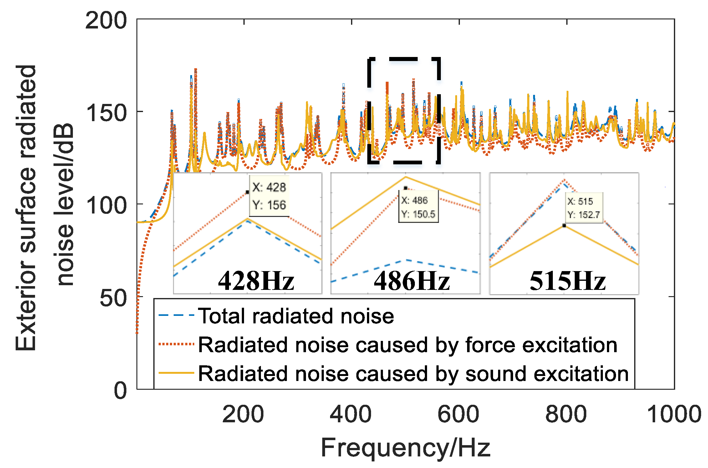
2.1. Analysis of the Vibration and Sound Characteristics of Cabin Structures under Hybrid Excitation

In this section, the sound field characteristic in the cabin is expressed by the mean square sound pressure near the inner surface of the cabin, the vibration characteristic of the cabin structure is expressed by the mean square vibration velocity of the cabin’s inner surface, and the sound radiation characteristic of the cabin structure is expressed by the radiated sound power of the exterior surface of the cabin.

The mean square sound pressure inside the cabin is calculated as follows:

$$P=\frac{{\displaystyle \underset{s}{\int }{P}_{\mathrm{in}}\left(z,\theta ,R\right)\ast {\overline{P}}_{\mathrm{in}}\left(z,\theta ,R\right)}ds}{S}$$

(1)

where $P_{\mathrm{in}}$ is the sound pressure near the interior surface of the cabin and S is the internal surface area.

The mean square vibration velocity of the cabin surface is calculated as follows:

$$V=\frac{{\displaystyle \underset{s}{\int }{V}_{\mathrm{in}}\left(z,\theta ,R\right)\ast {\overline{V}}_{\mathrm{in}}\left(z,\theta ,R\right)}ds}{S}$$

(2)

where $V_{\mathrm{in}}$ is the radial vibration velocity of the surface inside the cabin and S is the internal surface area.

The calculation expression of radiated sound power is shown as follows:

$$W=\frac{1}{2}\mathrm{Re}\left\{{\displaystyle \underset{s}{\int }{P}_{out}\left(M\right)V_r^{*}\left(M\right)}ds\right\}$$

(3)

In order to simplify the calculation model, a single-layer cylindrical shell was selected as the research object. A cylindrical coordinate system was established with the center of the left end face of the cabin as the origin of the coordinates, as shown in Figure 1. The length of the cylindrical shell L = 2.3 m, the radius R = 0.8 m, and the thickness of the cylindrical shell hs = 0.008 m. The Young’s modulus of the shell E = 2.1 × 10¹¹ N/m², the Poisson’s ratio $\mathsf{\sigma }=0.3$, and the density of the shell material ρ_s = 7800 kg/m³. The interior of the shell is air, the density ${\rho }_0=1.29$ kg/m³, the sound speed $c_0=340$ m/s, the outer part of the shell is water, the density ρ_e = 1000 kg/m³, and the sound speed c_e = 1500 m/s. Two excitation sources are arranged inside the cabin. The coordinate of the sound source is $\left(0.5R_0,0,0.5L_0\right)$, the sound pressure amplitude at a distance of 1 m from the sound source in the free field is 1 Pa, the coordinate of the force source is $\left(R_0,0,0.5L_0\right)$, and the excitation strength is 1 N. The initial condition is 0 state, and the boundary conditions at both ends of the single-layer cylindrical shell are simply supported. For the structure shown in Figure 1, the vibration equation of its shell is as follows:

$$\left[L\right]\left\{u\right\}=\frac{R_{}^2\left(1-v^2\right)}{E{h}_{}}\left\{-\left\{F\right\}\right\}$$

(4)

The constitutive equation of the sound cavity is as follows:

$$p(r,\omega )\equiv {\displaystyle {\int }_V{G}_0}(r,r^{\prime },\omega )\tilde{s}(r^{\prime },\omega )d{r}^{\prime }$$

(5)

Firstly, the structural vibration characteristics under the excitation of the sound source and force source were analyzed, as shown in Figure 2. When the sound source excitation is 1 Pa and the force source excitation intensity is 1 N, the sound field in the cabin is mainly determined by the sound source excitation, and the sound field monitoring in the cabin mainly reflects the sound source excitation information. The vibration characteristics of the cabin surface are mainly determined by the force source in the middle- and low-frequency bands, and the vibration of the shell caused by the sound source gradually increases with the increase in the frequency.

Force sources with different amplitudes were used for the excitation, so that the radiated sound power of the cabin was the same in each one-third octave frequency band under the excitation of the sound sources. The blue box is the amplitude of the equal potency source within each one third octave, and the red box is the amplitude of the equal potency source within the entire frequency band. As can be seen from Figure 3, the intensity of the external radiated noise caused by sound sources in the whole frequency band is similar to that of about 0.8 N of force source excitation. The amplitude of the equivalent point force source in the middle- and low-frequency bands is larger than that in the higher-frequency band, which shows that the influence of the sound source excitation on the radiation noise outside the cabin is more obvious in the middle- and low-frequency bands.

Furthermore, to analyze the coupling components in the vibration and acoustic sampling information, the sound monitoring information $P(\omega )$ and vibration monitoring information $V(\omega )$ can be decomposed into the following forms:

$$\begin{array}{l}P=P_P+P_V\\ V=V_P+V_V\end{array}$$

(6)

where $P_P$ is the acoustic monitoring information attributed to the sound source excitation, $P_V$ is the acoustic monitoring information attributed to the force source excitation, $V_P$ is the vibration monitoring information attributed to the sound source excitation, and $V_V$ is the vibration monitoring information attributed to the force source excitation. The sound monitoring information signal-to-interference ratio (PSIR) and vibration monitoring information signal-to-interference ratio (VSIR) are defined by the following expressions:

$$\begin{array}{l}\mathrm{PSIR}=20\lg \frac{P_P}{P_V}\\ \mathrm{VSIR}=20\lg \frac{V_V}{V_P}\end{array}$$

(7)

Based on the above conclusions, the 1.25 Pa sound source excitation and 1 N force source excitation were selected to work together in order to ensure the same radiation noise ability of the two excitation forms in the studied frequency band, and the two sets of monitoring information are shown in Figure 4. The PSIR is greater than 20 dB at most frequencies, indicating that the main component of acoustic monitoring information is caused by sound source excitation, while the coupling component caused by force source excitation accounts for a relatively small proportion. The VSIR decreases with the increase in frequency and is generally lower than that of acoustic monitoring information, and it is lower than 20 dB in some frequency bands below 400 Hz and above. Therefore, vibration monitoring information should be decoupled before radiation noise prediction.

2.2. Analysis of the Influence on Information Completeness of Acoustic and Vibration Monitoring Points

In this section, the completeness of the cabin structure information monitoring for different sampling points is discussed, providing a theoretical basis for the selection of the number of monitoring points. Equal intervals of the interior and exterior surfaces of the cabin structure were divided into M × N face elements (axial N and circumferential M), as shown in Figure 5. The information collected at the center position of each panel approximately represents the information of the whole panel, the collected information of the internal sound field is the sound pressure near the inner cabin surface, the collected information of the vibration is the vibration velocity on the inner cabin surface, and the collected information of the external sound field is the sound pressure near the outer cabin surface. Finally, the sound and vibration information of the whole cabin structure is obtained.

In order to ensure the complete monitoring information in the full frequency band, the monitoring points should be arranged according to the spatial sampling theorem, which requires half of the wavelength corresponding to the highest frequency as the monitoring point spacing. However, this scheme requires a large number of monitoring points and brings in more redundant information in the low-frequency band. We calculated the average error of the full frequency band of the information collected by each physical field under different numbers of monitoring points, as shown in Figure 6. To ensure that the sampling information can effectually reflect the real acoustic and vibration characteristics of the cabin structure, the number of internal acoustic field collection points should be greater than 9 in the circumference and 5 in the axial direction; the number of collection points on the cabin surface should be more than 15 in the circumference and 6 in the axial direction. As the external sound field is affected by both acoustic and force excitations, the distribution of the sound field is complex; therefore, the number of measurement points is large. Regarding the number of external sound field acquisition points, the numbers of circumferential and axial points should be greater than 15 and 9, respectively. When the number of sampling points is greater than that in this scheme, the effect of improving the completeness of the collected information is limited. To reduce monitoring costs and improve the prediction speed, the monitoring scheme should be selected based on the following conclusions of this section in the radiation noise prediction.

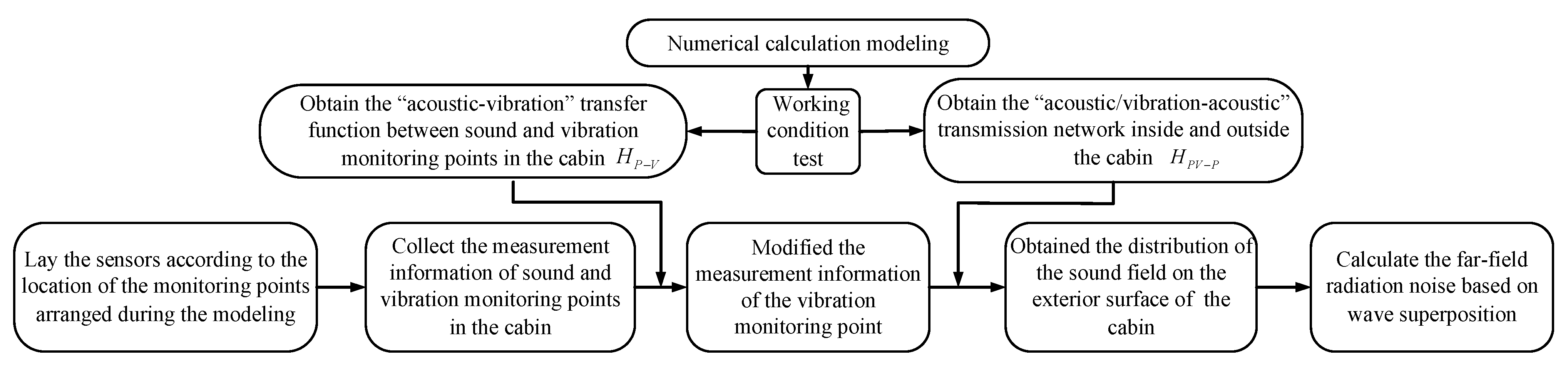
3. Underwater Radiation Noise Prediction Method for Cabin Structures

3.1. “Acoustic/Vibration-Acoustic” Transmission Network inside and outside the Cabin Structure Modeling Method Based on OTPA

OTPA can obtain the “acoustic/vibration-acoustic” transmission network inside and outside the cabin through the working condition test, and based on this transmission network and its monitoring data, the near-field radiation noise of the conformal hologram surface outside the cabin can be calculated in real time. For the application scenario where the positions of the input point and the output point are determined, the OTPA method can set the intermediate node of the transmission path between the excitation source and the target point under the actual operating conditions, collect the information of the intermediate node and the target point, and use the transfer function between the intermediate node and the target point to characterize each transmission path. This method can calculate the response of the target output point quickly and accurately, making it very suitable for the application scenario of this paper.

OTPA was originally an analysis method based on experimental testing. In recent years, with the development of computer technology, CAE-based OTPA numerical calculation methods have replaced real experimental testing in some application scenarios, reducing the test costs and the complexity of the test systems to a certain extent. The transfer network constructed in this paper can be tested by experimental or numerical calculation, and the two can also be combined. Since the structure of the simulation and test object is known and relatively simple, in order to facilitate the discussion of the problem, this paper adopts the CAE-based numerical method to model the “sound/vibration-sound” transmission network of the cabin structure.

The input signal of the sound source excitation is as follows:

$$p\left(\omega ,t\right)=A_p\ast \exp (j\omega t+{\phi }_p)$$

(8)

where $A_p$ is the amplitude of the acoustic excitation signal and ${\varphi }_p$ is the phase of the acoustic excitation signal.

The input signal of the force source excitation is as follows:

$$v\left(\omega ,t\right)=A_v\ast \exp (j\omega t+{\phi }_v)$$

(9)

where $A_v$ is the amplitude of the force excitation signal and ${\varphi }_v$ is the phase of the force excitation signal.

When the numerical working condition test is carried out, the working condition test model is established using the numerical calculation software COMSOL 6.0. Secondly, the excitation input amplitude $A_p$ and phase ${\varphi }_p$ of the sound source and the excitation input amplitude $A_v$ and phase ${\varphi }_v$ of the force source are calculated in the studied frequency band to obtain the acoustic monitoring data of the acoustic monitoring points inside the cabin, the vibration monitoring data of the vibration monitoring points, and the acoustic response data of the near-field radiation noise response points on the conformal holographic plane outside the cabin, which is a working condition test. Finally, multiple working condition tests are carried out by changing the relative size of $A_p$ and $A_v$ and the relative phase of ${\varphi }_p$ and ${\varphi }_v$.

According to the conclusions in Section 2.1, in the vibration–acoustic synchronous monitoring information, the PSIR has a relatively high reliability and is more than 20 dB in most of the frequency bands. The vibration and acoustic information has a large energy difference, so the acoustic information can be approximated as independent excitation of the sound source, while the vibration information has strong coupling. Therefore, the “acoustic-vibration” transfer function $H_{P-V}(\omega )$ between the monitoring points inside the cabin can first be constructed by conducting numerical condition tests, and then the acoustic information is used as a reference to solve the coupling part triggered by the sound source in the vibration information, as shown in Equation (10):

$$A_0(\omega )=P(\omega )H_{P-V}(\omega )$$

(10)

where $A_0(\omega )$ is the coupling part triggered by the sound source in the vibration information and $P(\omega )$ is the acoustic information.

The vibration monitoring information is decoupled as shown in Equation (11):

$$A(\omega )=A_q(\omega )-A_0(\omega )$$

(11)

where $A_q(\omega )$ is the vibration information and $A(\omega )$ is the vibration information after decoupling.

Based on the assumption that the system is linear and time-invariant, the response function of the response point can be expressed as follows:

$$Y(\omega )=X(\omega )H_{PV-P}(\omega )$$

(12)

where $Y(\omega )$ is the acoustic output vector of the target point, $X(\omega )$ is the vibration and acoustic input vector of the monitoring point, and $H_{PV-P}(\omega )$ is the “acoustic/vibration-acoustic” transmission network inside and outside the cabin structure. The input vector is the combination of the sound pressure signal and vibration signal, and the sound output vector is the sound pressure signal. By measuring the physical quantities of the vibration and acoustic monitoring points and target points under the numerical operation conditions of the cabin structure system, the sample matrix of the monitored excitation input and target response output can be constructed:

$$\left(\begin{array}{cccccc}{A}_{11}& \cdots & A_{1k}& P_{11}& \cdots & P_{1m}\\ A_{21}& \cdots & A_{2k}& P_{21}& \cdots & P_{2m}\\ A_{31}& \cdots & A_{3k}& P_{31}& \cdots & P_{3m}\\ A_{41}& \cdots & A_{4k}& P_{41}& \cdots & P_{4m}\\ ⋮& \cdots & ⋮& ⋮& \cdots & ⋮\\ A_{n1}& \cdots & A_{nk}& P_{n1}& \cdots & P_{nm}\end{array}\right)\left(\begin{array}{c}{H}_{a1}\\ ⋮\\ H_{ak}\\ H_{p1}\\ ⋮\\ H_{pm}\end{array}\right)=\left(\begin{array}{c}{Y}_1\\ Y_2\\ Y_3\\ Y_4\\ ⋮\\ Y_n\end{array}\right)$$

(13)

where n represents the number of test conditions, k and m represent the numbers of vibration and harmonic reference points, respectively, $Y_n$ represents the target reference point response of the NTH working condition, $a_{nk}$ represents the response of the KTH vibration reference point under the NTH working condition, $p_{nm}$ represents the response of the MTH acoustic reference point under the NTH working condition, $H_{ak}$ represents the transfer rate of the KTH vibration reference point to the target point, and $H_{pm}$ represents the transfer rate of the MTH acoustic reference point to the target point.

According to the above formula, the numerical working condition transfer matrix of the cabin structural system can be solved:

$$\left(\begin{array}{c}{H}_{a1}\\ ⋮\\ H_{ak}\\ H_{p1}\\ ⋮\\ H_{pm}\end{array}\right)={\left(\begin{array}{cccccc}{A}_{11}& \cdots & A_{1k}& P_{11}& \cdots & P_{1m}\\ A_{21}& \cdots & A_{2k}& P_{21}& \cdots & P_{2m}\\ A_{31}& \cdots & A_{3k}& P_{31}& \cdots & P_{3m}\\ A_{41}& \cdots & A_{4k}& P_{41}& \cdots & P_{4m}\\ ⋮& \cdots & ⋮& ⋮& \cdots & ⋮\\ A_{n1}& \cdots & A_{nk}& P_{n1}& \cdots & P_{nm}\end{array}\right)}^{-1}\left(\begin{array}{c}{Y}_1\\ Y_2\\ Y_3\\ Y_4\\ ⋮\\ Y_n\end{array}\right)$$

(14)

To accurately obtain the transfer matrix of the system, it is necessary to select a reasonable working condition to test the system. To ensure the uniqueness of the matrix inversion in Equation (14), the principle of $n>k+m$ should be satisfied.

Formula (14) is expressed as follows:

$$H_{PV-P}=X^{+}Y$$

(15)

where $X^{+}$ is the generalized inverse matrix of X.

Because there is usually correlation between each condition when testing the numerical condition, the direct inversion of X will lead to incorrect results. In order to avoid the above situation, the singular value decomposition of the transfer matrix is carried out. The singular value decomposition of X can be expressed as follows:

$$X=U\Sigma V^{\mathrm{T}}$$

(16)

where U and V are unitary matrices, $\Sigma$ is a nonnegative diagonal matrix with singular values arranged in descending order, and $\mathrm{T}$ is a conjugate transpose matrix.

Through generalized inverse calculation of Equation (16) and substitution into Equation (15), we can get

$$H_{PV-P}=V{\Sigma }^{-1}{U}^{\mathrm{T}}Y$$

(17)

where ${\Sigma }^{-1}$ is the inverse of the square matrix $\Sigma$.

3.2. Underwater Radiation Noise Prediction Method Based on the Wave Superposition Method

The wave superposition method only needs to obtain the sound field distribution on the outer surface of the cabin structure to calculate the radiation noise at any position in the far field. The basic principle is to configure several equivalent point sound sources inside the structure, generally monopole or dipole sources. The source intensity of the configured equivalent source is calculated using the sound field distribution on the external surface of the structure. Finally, the radiation sound field of the structure is calculated by the linear superposition of the radiation sound field of the equivalent source.

The radiated sound pressure of a series of simple sound sources located inside the structure at a field point r in space can be expressed as follows:

$$p\left({\overrightarrow{r}}_m\right)={\displaystyle {\int }_{R}j{\rho }_e{c}_{e}kq\left({\overrightarrow{r}}_0\right)G\left({\overrightarrow{r}}_m,{\overrightarrow{r}}_0\right)}dR \left(m=1,2,\cdots M\right)$$

(18)

where ${\rho }_e$ is the fluid density, $c_e$ is the speed of sound,$k$ is the wave number, $q\left({\overrightarrow{r}}_0\right)$ is the source intensity of the simple source inside the structure, and $G\left({\overrightarrow{r}}_m,{\overrightarrow{r}}_0\right)$ is the Green’s function between point $r_m$ and $r_0$ under free-field conditions, which can be expressed as follows:

$$G\left({\overrightarrow{r}}_m,{\overrightarrow{r}}_0\right)=\frac{e^{jkr}}{4\pi r}$$

(19)

where $r$ is the distance between the prediction point and the simple source, $r=\left|{\overrightarrow{r}}_m-{\overrightarrow{r}}_0\right|$.

By matching the external surface radiation sound pressure of the structure, the simple source strength configured in the structure can be solved, which can be expressed in a matrix form as follows:

$$Y_H=G_{H}Q$$

(20)

where $Y_H$ is the response matrix of measuring points on the surface outside the structure,$G_H$ is the Green’s function from the equivalent source point to the measuring point on the surface outside the structure under the free-field condition, and $Q$ is the equivalent stream to be solved. With the help of the singular value decomposition method, it can be expressed as follows:

$$Q=V{\Sigma }^{-1}{U}^{\mathrm{T}}{P}_H$$

(21)

where $G_H=U\Sigma V^{\mathrm{T}}$.

3.3. Simulation Calculation and Analysis

The information processing flow diagram of the underwater radiation noise prediction method for cabin structures in this paper is shown in Figure 7:

Based on the numerical calculation software COMSOL 6.0, the research object described in Section 2.1 was numerically modeled, the relative amplitude and phase of the sound and force excitations were changed, and a total of 500 numerical condition tests were carried out. It is necessary to ensure that the radiation noise power of two excitation sources is the same when checking the prediction accuracy of radiation noise. Based on the research results in Section 2.1, a 1 N point force source and a 1.25 Pa point sound source were selected to work together. Based on the research results in Section 2.2, 15 × 6 = 90 vibration monitoring points and 9 × 5 = 45 acoustic monitoring points were uniformly arranged inside the cabin, and 15 × 9 = 135 acoustic response points were selected outside the cabin.

3.3.1. Modeling Accuracy Analysis of the “Acoustic/Vibration-Acoustic” Transmission Network inside and outside the Cabin Structure

Figure 8 shows the forecast results of the mean square sound pressure of noise on the outer cabin surface. The prediction accuracy of functional modeling based on synchronous vibration and acoustic monitoring is higher than that based on vibration monitoring, and the prediction error of the mean square sound pressure of noise outside the cabin is less than 0.5 dB in the studied frequency band. The error of the prediction accuracy of the functional modeling based on vibration monitoring increases obviously at some specific frequency points in the middle-frequency band. Figure 9 shows the radiated noise on the exterior surface of the cabin caused by different excitation forms, and the total radiated noise curve in the figure is the true value curve of radiated noise in Figure 8a. Combined with Figure 8b and Figure 9, it can be seen that if the radiation noise caused by the two excitation forms is in the opposite phase at the characteristic frequency, the transfer function modeling based on vibration monitoring is prone to producing large errors, which is generally consistent with the research conclusions in Section 2.1. Therefore, only monitoring vibration information under hybrid excitation will miss the radiation noise information generated by the sound source.

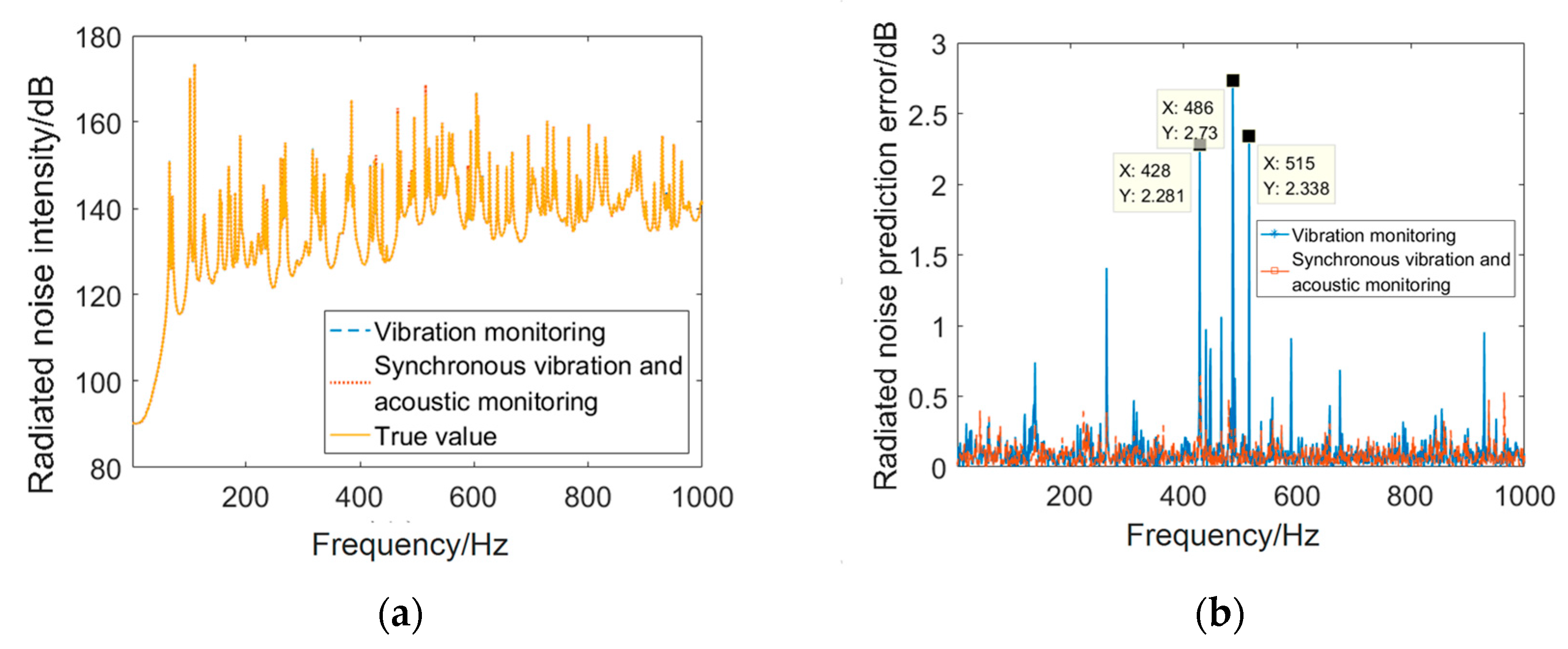
3.3.2. Performance Analysis of Far-Field Radiation Noise Prediction outside the Cabin

The coordinates of the observation point are $(100,0,L/2)$. As shown in Figure 10, the prediction error of radiation noise gradually increases with the increase in the frequency, and the average prediction error of far-field radiation noise in the one third octave band in the 1 kHz band is less than 4 dB. Compared with vibration monitoring, synchronous monitoring can significantly improve the prediction accuracy of underwater radiation noise, especially in the low-frequency band below 500 Hz. In the high-frequency band above 500 Hz, the sound excitation causes lower radiated sound power, and the underwater radiated noise is mainly caused by the force source excitation, so the prediction performance of the synchronous monitoring is essentially consistent with that of the vibration monitoring. It can be seen from the simulation results that the prediction accuracy of underwater radiation noise of the cabin structure under hybrid excitation can be effectively improved by adding acoustic monitoring points.

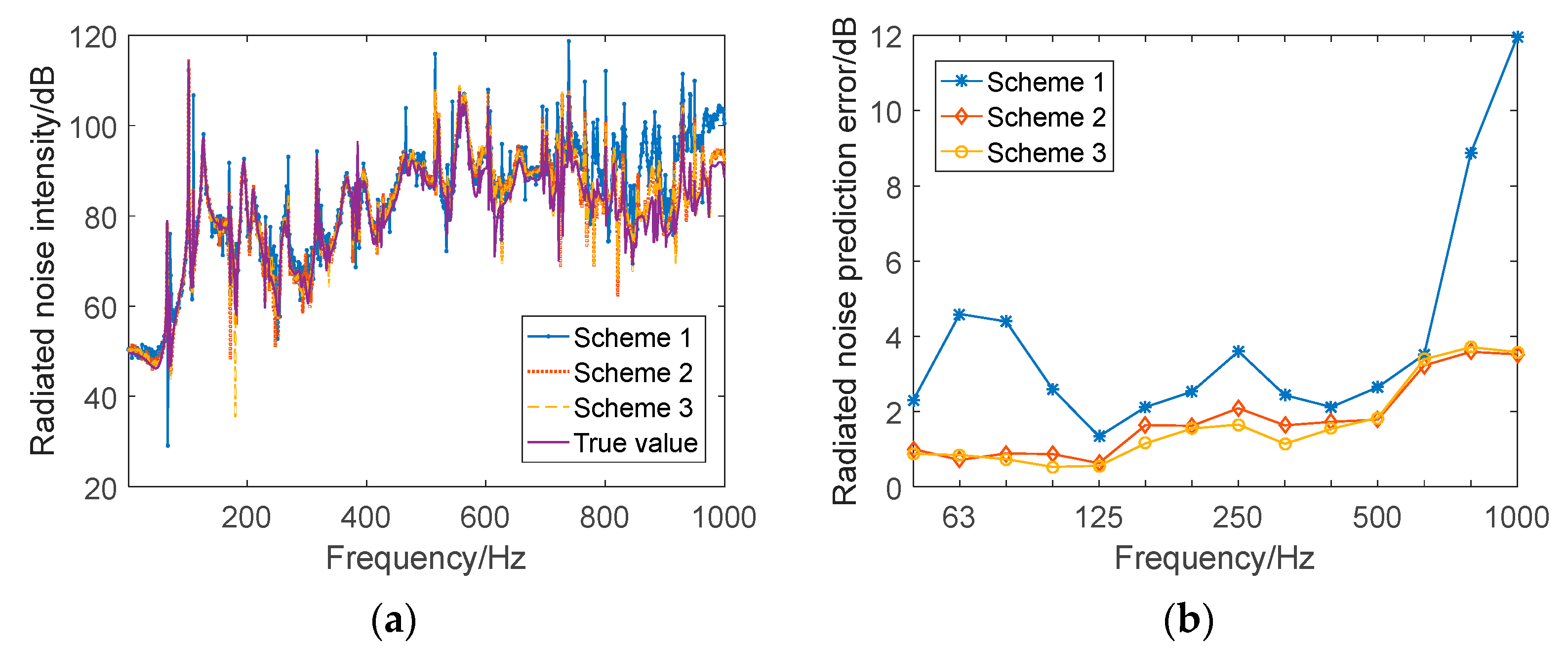
3.3.3. Comparative Analysis of Underwater Radiation Noise Prediction Performance under Different Monitoring Schemes

Three monitoring schemes were set in the simulation, as shown in

Table 1. Monitoring schemes.

Monitoring Scheme No.	Vibration Monitoring Point		Acoustic Monitoring Point
	Circumferential Number	Axial Number	Circumferential Number	Axial Number
Scheme 1	9	5	5	3
Scheme 2	15	6	9	5
Scheme 3	20	8	15	6

. The prediction results of underwater radiated noise are shown in Figure 11.

It can be seen that the prediction error of Scheme 1 is greater than that of Scheme 2 and Scheme 3, indicating that the monitoring information of vibration and sound inside the cabin of Scheme 1 is missing or incomplete. However, the noise prediction performance of Scheme 3 is not significantly improved compared with Scheme 2, indicating that the vibration and acoustic monitoring information of Scheme 2 and Scheme 3 is essentially complete, and that continuing to add vibration and sound monitoring points has little significance for improving the prediction accuracy of underwater noise, which is essentially consistent with the research conclusions in Section 2.2.

3.3.4. Analysis of the Influence of External Sound Response Points on Underwater Radiation Noise Prediction Performance

Three sound response point schemes were set, namely, 9 × 5, 15 × 9, and 24 × 11. The calculation results are shown in Figure 12. When the number of sound response points on the external surface of the cabin is increased, the prediction accuracy of underwater radiated noise is significantly improved. However, when the number of sound response points on the holographic surface is increased from 135 to 264, the prediction accuracy of underwater radiated noise is limited, indicating that the monitoring information of Scheme 3 is essentially complete, which is generally consistent with the research conclusions in Section 2.2.

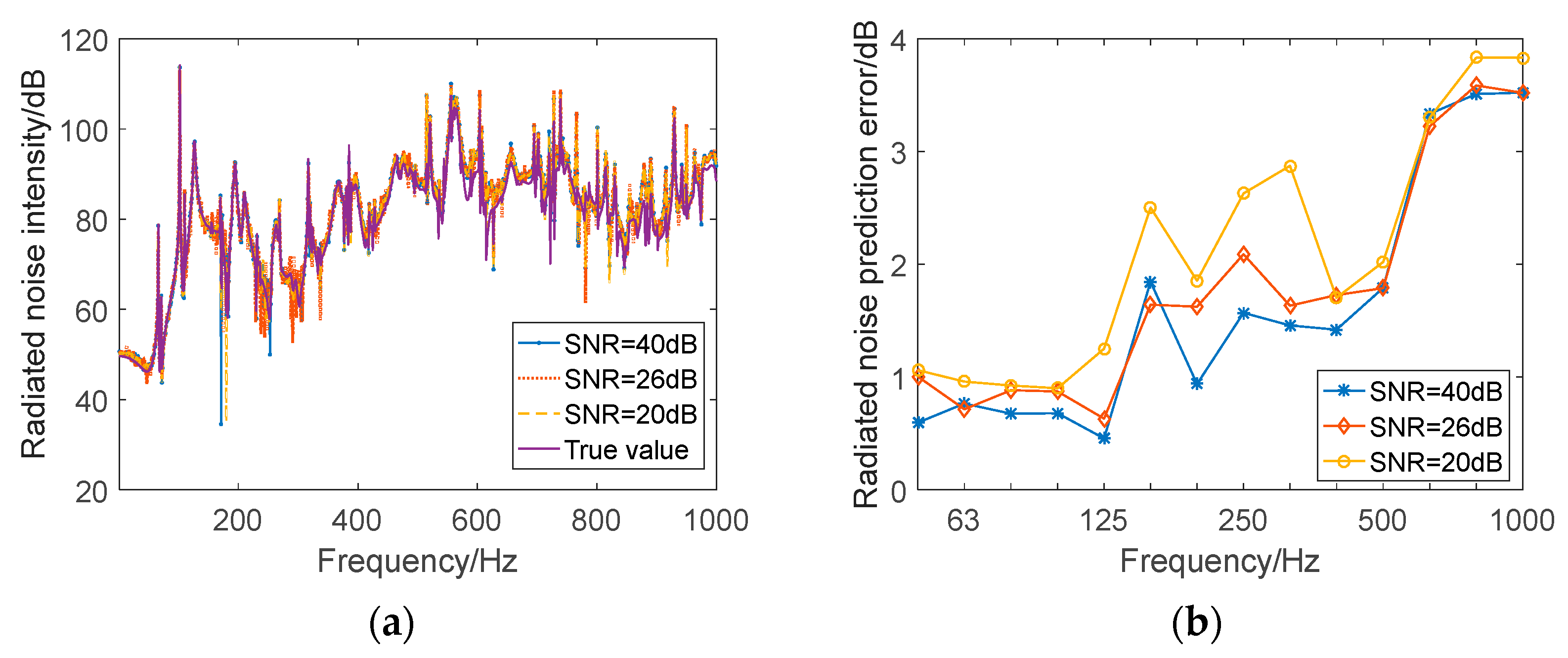
3.3.5. Analysis of the Influence of Underwater Radiation Noise Prediction Performance under Different SNR Conditions

The SNR is defined by

$$SNR=20\lg (\frac{E_S}{E_N})$$

(22)

where $E_S$ is the monitor signal strength and $E_N$ is the introduced noise intensity.

A random noise of 1%, 5%, and 10%, of the signal strength is added to each monitoring signal. The corresponding SNRs are 40, 26, and 20 dB, respectively. Figure 13 shows the forecast results of radiated noise under various SNRs. It can be seen that when the SNR is reduced from 40 dB to 20 dB, the accuracy of the radiation noise prediction does not decrease significantly. When the SNR is 20 dB, the average prediction error of radiation noise in the 1/3 oct band can be controlled within 4 dB, and that in the low-frequency band can be controlled within 1 dB.

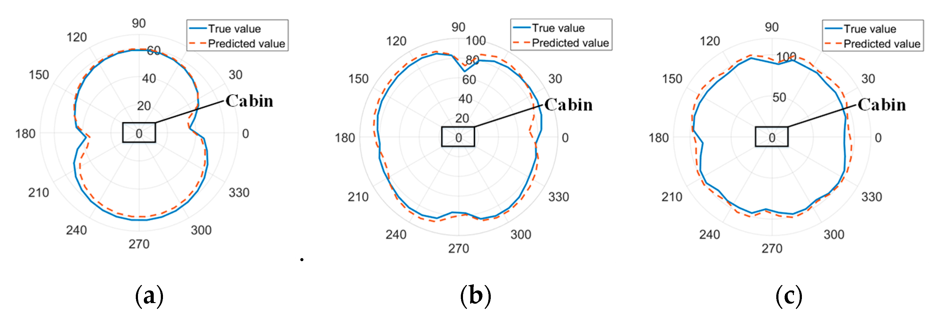
3.3.6. Performance Analysis of Spatial Directional Prediction of Underwater Radiated Noise

Figure 14 shows the radiation noise prediction results of each point on the circle 100 m away from the cabin. The circle is on the horizontal plane, its center is the geometric center of the cabin, and the angle interval is 10°. When the prediction frequency is 100 Hz, the prediction error of radiation noise in each direction is controlled within 1 dB. With the increase in the prediction frequency, the prediction error of radiation noise increases gradually. In addition, the radiation noise prediction accuracy is higher in the range of ±60° in the positive transverse direction of the cabin.

4. Experiments

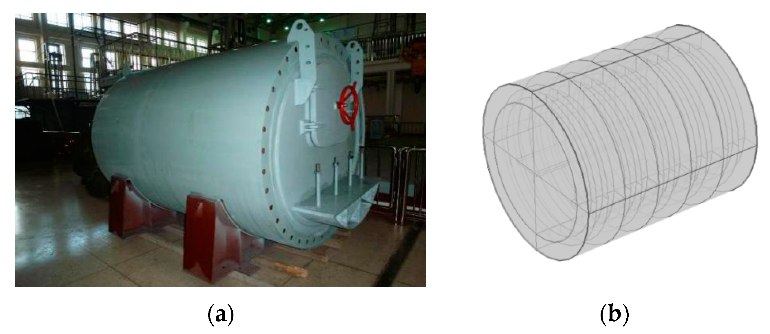
4.1. Experimental Conditions

The test object is a submarine cabin shrinkage model, the cabin model is a double-shell structure, and the pressure hull is an outer frame form. The length of the main double-shell section $L=$2300 mm, the light shell radius $R_1=$2000 mm, the pressure shell radius $R_2=$1600 mm, ballast devices are arranged at both ends, and four solid ribs and ten ring ribs are distributed at equal intervals between the inner and outer shells. The test objects are shown in Figure 15a, while the finite element model is shown in Figure 15b.

A shaker and air sound source were arranged in the cabin model as the excitation equipment. The sound source excitation was a sound box, 13 cm long, 11 cm wide, 18 cm high, and with 8 cm diameter of the circular radiant surface. The shaker model was JZ-50, the frequency band was 50~3000 Hz, and the maximum excitation force was 500 N. The excitation signals of the two excitation devices were single-frequency signals (1/3 octave point within 100 Hz–1 kHz). A column coordinate system was established with the center of the left end face of the cabin model as the origin of the coordinates. The coordinate of the acoustic excitation source was $\left(0,0,L/2\right)$, while the coordinate of the force excitation source was $\left(R_2/2,0,L/2\right)$. The collector model was B&K3660-D, and the front section of the collector was set with a high-pass digital filter with an upper frequency of 7 Hz. The sampling rate of the collector was 12.8 × 2.56 kHz. The hydrophone type was B&K8103, the vibration sensor type was PCB M352C68, and the microphone type was MP201.

Inside the cabin, the measuring points were numbered in a clockwise sequence (from the watertight door end to the cabin), and a microphone and vibration sensor were arranged at each measuring point. The positions of the measuring points on different sections of the shell were represented by the letters A–E. The positions of different measuring points on the same section were represented by numbers. There were 40 microphones and 40 vibration sensors arranged in the cabin, as shown in Figure 16ab. Four far-field investigation points were set in the underwater acoustic field, as shown in Figure 16c. The coordinates of investigation points 1–4 are $\left(6,0,L/2\right)$, $\left(11,0,L/2\right)$, $\left(6,0,L/2-3\right)$, and $\left(6,0,L/2+3\right)$, respectively.

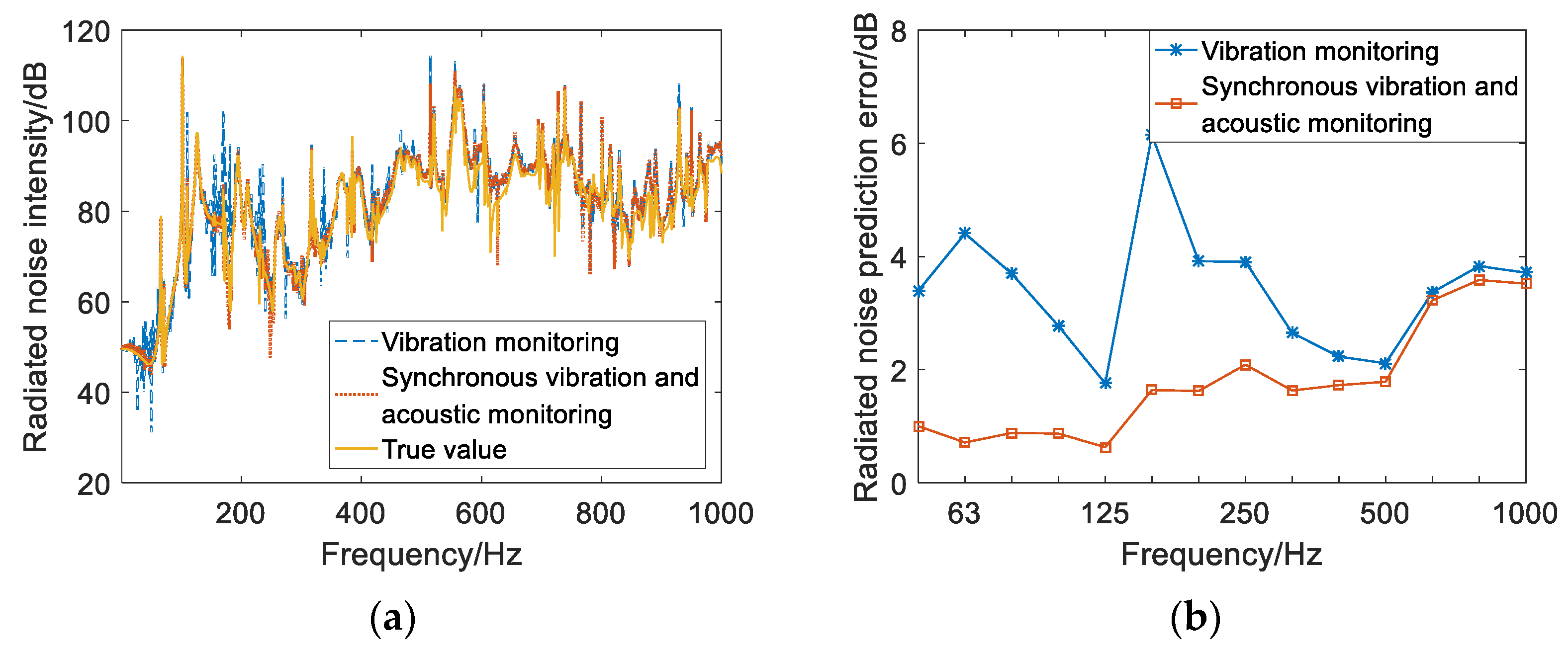
4.2. Analysis of Experimental Results

In this study, the “acoustic/vibration-acoustic” transmission network inside and outside the cabin structure of the cabin model was numerically modeled by using the numerical calculation software COMSOL 6.0. Figure 17 shows the real and predicted values of radiation noise at four far-field radiation noise detection points, while

Table 2. Radiation noise prediction error.

Frequency (Hz)	Radiation Noise Prediction Error (dB)
	Investigation Point 1		Investigation Point 2		Investigation Point 3		Investigation Point 4
	Vibration Monitoring	Synchronous Monitoring	Vibration Monitoring	Synchronous Monitoring	Vibration Monitoring	Synchronous Monitoring	Vibration Monitoring	Synchronous Monitoring
100	8.54	4.87	6.28	3.43	7.24	3.74	8.59	3.5
125	6.49	3.49	7.92	2.68	4.65	4.87	5.06	3.66
160	4.67	0.57	9.46	2.97	4.1	4.29	4.1	0.04
200	3.19	0.52	5.86	2.76	3.53	4.11	0.85	0.52
250	3.42	2.53	6.38	3.01	3.2	0.44	7.38	1.76
315	3.98	1.91	5.3	2.26	6.18	0.44	7.28	0.08
400	3.06	2.44	8.13	4.99	7.14	0.33	3.34	2.68
500	2.19	1.88	3.14	0.46	4	2.01	5.57	2.54
630	4.99	1.88	2.6	1.18	5.43	1.76	2.95	0.28
800	5.66	2.33	6.26	2.78	2.04	0.73	3.73	3.1
1000	3.75	1.76	5.23	2.81	3.42	3.62	4.37	1.16

shows the radiation noise prediction error table based on two monitoring methods at each observation point. The frequency points are the excitation frequencies of the sound source and the force source, which were selected according to one-third octave points in the 100 Hz–1 kHz frequency band. It can be seen that the underwater radiated noise prediction method proposed in this paper can accurately predict the radiated noise of the cabin model. Under the force–acoustic hybrid excitation, the prediction accuracy of the model for underwater radiated noise is higher when using the vibration–acoustic synchronous monitoring scheme. Moreover, the forecast error tendency increases with the increase in frequency, which is essentially consistent with the simulation results. The prediction error of the model for underwater radiated noise based on vibration and acoustic monitoring is less than 5 dB in the frequency band below 1 kHz. Investigation point 3 and investigation point 4 are in a symmetric position relative to the structure, and it can be seen that the prediction accuracy of radiation noise is similar in the overall trend.

5. Conclusions

Aiming at the engineering limitations of traditional ship vibration online monitoring and noise prediction methods, we first studied the vibration and sound characteristics of the cabin structure under the hybrid excitation of force and sound and the coupling characteristics of vibration and acoustic monitoring information theoretically. On this basis, we propose a method of underwater radiation noise prediction for cabin structures based on synchronous vibration and acoustic monitoring combined with OTPA and the wave superposition method. This method solves the problem of missing radiation noise caused by sound excitation in traditional vibration monitoring by adding acoustic monitoring points inside the cabin. Compared with the prediction results of the traditional vibration monitoring method, it was found that the proposed method can effectively improve the prediction accuracy of the underwater radiation noise of the cabin structure, and the prediction accuracy is more obvious in the middle- and low-frequency bands. The forecast error of radiation noise increases with the increase of frequency, but the average forecast error of the one third octave band below 1kHz is less than 4dB. In addition, the proposed method can predict the radiation noise at any position in the far field of the ship cabin structure, which makes up for the limitations of the traditional OTPA method. The effectiveness of the proposed method was further verified by the model test of the tank section. In addition, practical problems such as the noise prediction of multi-cabin structures and the optimal arrangement of monitoring points need to be further studied in subsequent work.

References

1. Zhang, B.; Xiang, Y.; He, P.; Zhang, G.-J. Study on prediction methods and characteristics of ship underwater radiated noise within full frequency. Ocean Eng. 2019, 174, 61–70. [Google Scholar] [CrossRef]
2. Ye, L.; Shen, J.; Tong, Z.; Liu, Y. Research on acoustic reconstruction methods of the hull vibration based on the limited vibration monitor data. Ocean Eng. 2022, 266, 112886. [Google Scholar] [CrossRef]
3. Badino, A.; Borelli, D.; Gaggero, T.; Rizzuto, E.; Schenone, C. Normative framework for ship noise: Present and situation and future trends. Noise Control Eng. J. 2012, 60, 740–762. [Google Scholar] [CrossRef]
4. Zheng, X.; Dai, W.; Qiu, Y.; Hao, Z. Prediction and energy contribution analysis of interior noise in a high-speed train based on modified energy finite element analysis. Mech. Syst. Signal Process. 2019, 126, 439–457. [Google Scholar] [CrossRef]
5. Yaylacı, M.; Avcar, M. Finite element modeling of contact between an elastic layer and two elastic quarter planes. Comput. Concr. Int. J. 2020, 26, 107–114. [Google Scholar]
6. Liu, Q.; Thompson, D.J.; Xu, P.; Feng, Q.; Li, X. Investigation of train-induced vibration and noise from a steel-concrete composite railway bridge using a hybrid finite element-statistical energy analysis method. J. Sound Vib. 2020, 471, 115197. [Google Scholar] [CrossRef]
7. Chen, L.L.; Lian, H.; Liu, Z.; Chen, H.B.; Atroshchenko, E.; Bordas, S. Structural shape optimization of three dimensional acoustic problems with isogeometric boundary element methods. Comput. Methods Appl. Mech. Eng. 2019, 355, 926–951. [Google Scholar] [CrossRef]
8. Wu, C.; Yin, H. The inclusion-based boundary element method (iBEM) for virtual experiments of elastic composites. Eng. Anal. Bound. Elem. 2021, 124, 245–258. [Google Scholar] [CrossRef]
9. Wu, Y.H.; Dong, C.Y.; Yang, H.S. Isogeometric indirect boundary element method for solving the 3D acoustic problems. J. Comput. Appl. Math. 2020, 363, 273–299. [Google Scholar] [CrossRef]
10. Vaitkus, D.; Tcherniak, D.; Brunskog, J. Application of vibro-acoustic operational transfer path analysis. Appl. Acoust. 2019, 154, 201–212. [Google Scholar] [CrossRef]
11. Li, R.; Bu, W.; Xu, R. Research on Ship-Radiated Noise Evaluation and Experimental Verification Based on OTPA Optimized by Operating Condition Clustering. J. Coast. Res. 2020, 111, 326–330. [Google Scholar] [CrossRef]
12. Wang, C.; Jiang, W. A novel transmissibility matrix method for identifying partially coherent noise sources on vehicles. Appl. Acoust. 2020, 165, 107318. [Google Scholar] [CrossRef]
13. Nan, Z.; Behrendt, M.; Lu, M.; Petersen, M.; Albers, A. OTPA method-based contribution analysis of components on the vibration of fuel cell in fuel cell vehicles. In Proceedings of the INTER-NOISE and NOISE-CON Congress and Conference Proceedings, Washington, DC, USA, 1–5 August 2021; Institute of Noise Control Engineering: Reston, VI, USA, 2021; Volume 263, pp. 3720–3730. [Google Scholar]
14. Rodríguez, P.V.; Magrans, F.X. OTPA method weakness in real case applications. In Proceedings of the INTER-NOISE and NOISE-CON Congress and Conference Proceedings, Washington, DC, USA, 1–5 August 2021; Institute of Noise Control Engineering: Reston, VI, USA, 2016; Volume 253, pp. 3261–3269. [Google Scholar]
15. Wang, B.; Tang, W.; Fan, J. An approximate method to acoustic radiation problems: Element Radiation Superposition Method. Chin. J. Acoust. 2008, 27, 350–357. [Google Scholar]
16. Chen, M.; Zhang, C.; Tao, X.; Deng, N. Structural and acoustic responses of a submerged stiffened conical shell. Shock. Vib. 2014, 2014, 954253. [Google Scholar] [CrossRef]
17. Gao, Y.; Yang, B.Q.; Shi, S.G.; Zhang, H.Y. Extension of sound field reconstruction based on element radiation superposition method in a sparsity framework. Chin. Phys. B 2022, 32, 044302. [Google Scholar] [CrossRef]
18. Koopmann, G.H.; Song, L.; Fahnline, J.B. A method for computing acoustic fields based on the principle of wave superposition. J. Acoust. Soc. Am. 1989, 86, 2433–2438. [Google Scholar] [CrossRef]
19. Jeans, R.; Mathews, I.C. The wave superposition method as a robust technique for computing acoustic fields. J. Acoust. Soc. Am. 1992, 92, 1156–1166. [Google Scholar] [CrossRef]
20. Bi, C.X.; Stuart Bolton, J. An Equivalent Source Technique for Recovering the Free Sound Field in a Noisy Environment. J. Acoust. Soc. Am. 2012, 131, 70–1260. [Google Scholar] [CrossRef] [PubMed]
21. Geng, L.; Zhang, X.Z.; Bi, C.X. Reconstruction of transient vibration and sound radiation of an impacted plate using time domain plane wave superposition method. J. Sound Vib. 2015, 344, 114–125. [Google Scholar] [CrossRef]
22. Yang, C.; Wang, Y.S.; Guo, H. Hybrid patch near-field acoustic holography based on Kalman filter. Appl. Acoust. 2019, 148, 23–33. [Google Scholar] [CrossRef]
Figure 1. Calculation model.
Applsci 13 12667 g001
Figure 2. Structural acoustic and vibration characteristics under force and sound excitation: (a) Mean square sound pressure. (b) Mean square vibration velocity. (c) Radiated sound power.
Applsci 13 12667 g002
Figure 3. Equivalent point force source amplitude.
Applsci 13 12667 g003
Figure 4. Sound and vibration monitoring information signal-to-interference ratio: (a) PSIR; (b) VSIR.
Applsci 13 12667 g004
Figure 5. Cabin structure information monitoring diagram.
Applsci 13 12667 g005
Figure 6. Average error of the full frequency band of the information collected by each physical field under different numbers of monitoring points: (a) Inner surface mean square sound pressure. (b) Internal surface mean square velocity. (c) Outer surface mean square sound pressure.
Applsci 13 12667 g006
Figure 7. Information processing flowchart for noise prediction.
Applsci 13 12667 g007
Figure 8. Modeling results of the “vibration/acoustic--acoustic” hybrid transfer function inside and outside the cabin structure: (a) Spectrum curve of surface noise outside the cabin. (b) Prediction error of surface noise outside the cabin.
Applsci 13 12667 g008
Figure 9. Surface radiation noise caused by different excitation forms outside the cabin.
Applsci 13 12667 g009
Figure 10. Prediction results of far-field radiated noise outside the cabin: (a) Far-field radiation noise spectrum. (b) Far-field radiation noise one third octave in-band mean error.
Applsci 13 12667 g010
Figure 11. Radiated noise prediction results under different monitoring schemes: (a) Far-field radiation noise spectrum. (b) Far-field radiation noise one third octave in-band mean error.
Applsci 13 12667 g011
Figure 12. Radiated noise prediction results of different response points on the exterior surface of the cabin: (a) Far-field radiation noise spectrum. (b) Far-field radiation noise one third octave in-band mean error.
Applsci 13 12667 g012
Figure 13. Radiated noise prediction results with different SNRs: (a) Far-field radiation noise spectrum. (b) Far-field radiation noise one third octave in-band mean error.
Applsci 13 12667 g013
Figure 14. Radiation noise predicted results at different angles: (a)100 Hz; (b) 630 Hz; (c) 1000 Hz.
Applsci 13 12667 g014
Figure 15. Tested cabin and its finite element model: (a) Cabin model. (b) Finite element model.
Applsci 13 12667 g015
Figure 16. Schematic diagram of the locations of the monitoring points and investigation points: (a) Cabin inner monitoring point (main view). (b) Cabin inner monitoring point (side view). (c) Far-field investigation point.
Applsci 13 12667 g016
Figure 17. Far-field radiation noise prediction results: (a) Investigation point 1. (b) Investigation point 2. (c) Investigation point 3. (d) Investigation point 4.
Applsci 13 12667 g017