
Shared Graph Neural Network for Channel Decoding


Abstract
:1. Introduction
- We share the same weights in GNN-based channel decoding algorithm especially in the update of factor nodes, variable nodes, factor-to-variable node messages, and variable-to-factor node messages.
- Based on different sharing schemes, we propose two shard GNN (SGNN)-based channel decoding algorithms to balance BER performance and storage complexity.
- Furthermore, we apply the SGNN-based channel decoding algorithm to BCH and LDPC decoders, which reduces the storage resources required by GNN-based channel decoders with a slight decrease in BER performance.
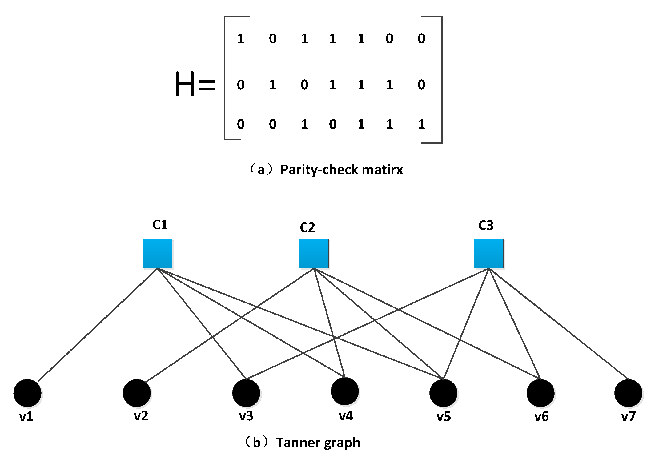
2. Preliminary
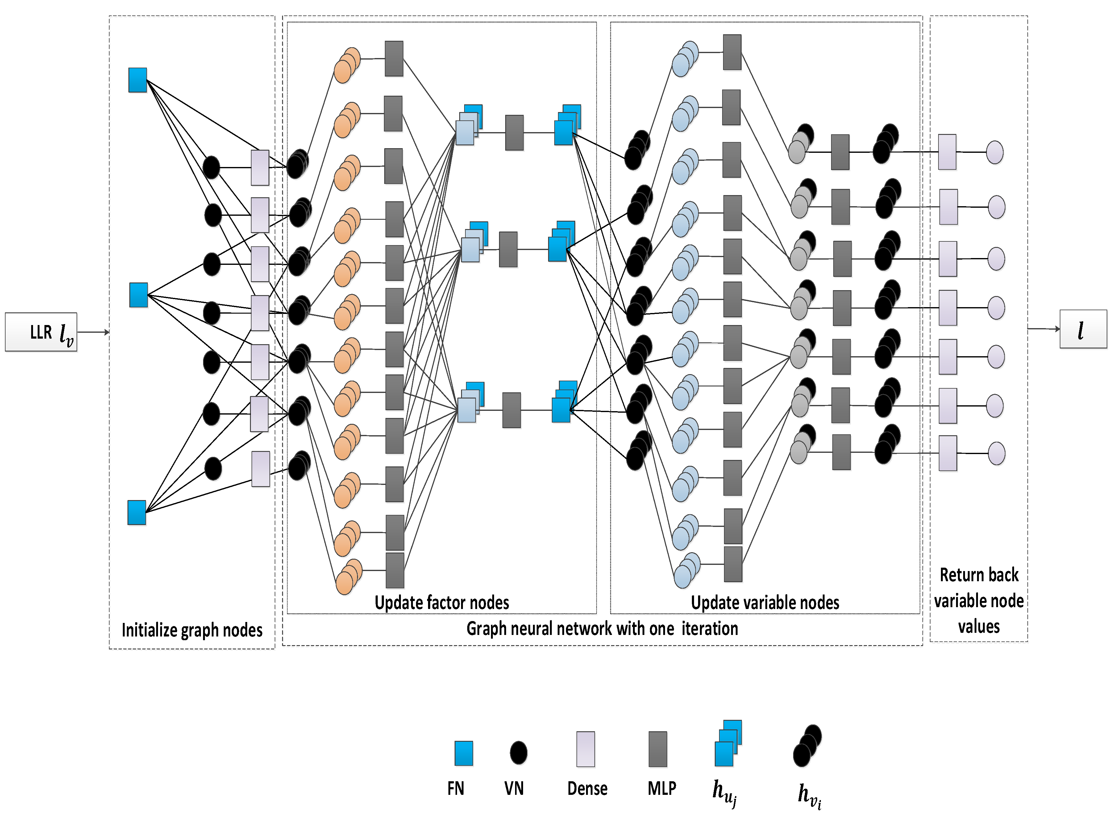
GNN-Based Channel Decoding
- Step 1:
- From the VN to FN, the message is passed in the graph aswhere denotes the parameters of the node, and the symbol denotes that the two tensors are concatenation together. The function maps messages to high-dimensional features by multiplying weights. Simple multilayer perceptrons (MLPs) are used to expand the dimension.
- Step 2:
- Update the FN value aswhere denotes the parameters in FN. We use aggregation similar to min-sum algorithm [24]. We may also use , , and operations, and the updated FN value is given by .
- Step 3:
- From the FN to VN, the message is passed in the graph aswhere denotes the trainable parameters in another direction edge.
- Step 4:
- Update the VN value aswhere denotes the parameters in VN. The decoding result is also output from this step. We may also use , , and operations, and the updated VN value is given by .
| Algorithm 1: GNN-based Channel Decoding Algorithm in ref. [22]. |
 |
3. SGNN Based Channel Decoding Algorithm
3.1. SGNN-Based Channel Decoding Algorithm 1
| Algorithm 2: The Proposed Shared GNN-based Channel Decoding Algorithm 1. |
 |
3.2. SGNN-Based Channel Decoding Algorithm 2
| Algorithm 3: The Proposed Shared GNN-based Channel Decoding Algorithm 2. |
 |
4. Simulation Results and Discussions
4.1. BCH Codes
4.2. Regular LDPC Code
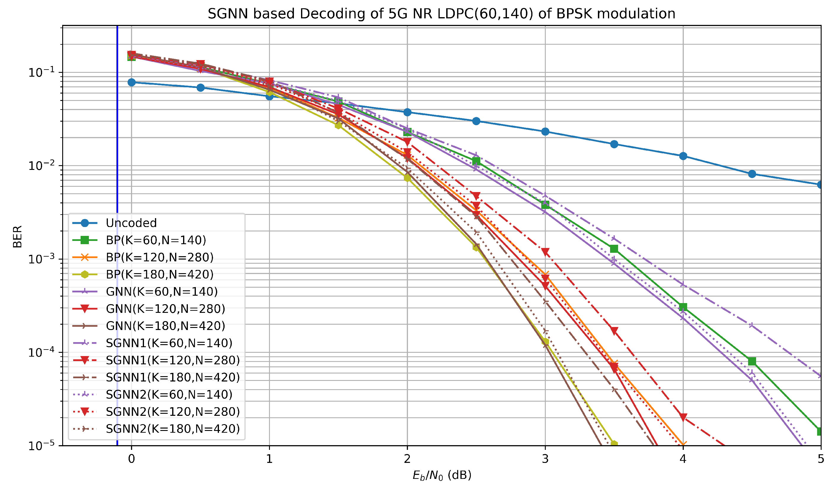
4.3. 5g NR LDPC Code
4.4. Complexity Analysis
5. Open Issues
- A possible way to implement a universal GNN-based channel decoder is to train GNN-based channel decoder weights for multiple forward error correction (FEC) parallel codes.
- The decoding complexity of the proposed SGNN is higher compared with that of BP, and other complexity reduction methods are put together to further reduce complexity, such as pruning, quantification, etc.
- Extensions to non-AWGN channels and other modulation methods are possible.
6. Conclusions
Author Contributions
Funding
Institutional Review Board Statement
Informed Consent Statement
Data Availability Statement
Conflicts of Interest
References
- Pak, M.; Kim, S. A review of deep learning in image recognition. In Proceedings of the 2017 4th International Conference on Computer Applications and Information Processing Technology (CAIPT), Kuta Bali, Indonesia, 8–10 August 2017; pp. 1–3. [Google Scholar]
- Shorten, C.; Khoshgoftaar, T.M. A survey on image data augmentation for deep learning. J. Big Data 2019, 6, 1–48. [Google Scholar] [CrossRef]
- Minaee, S.; Boykov, Y.; Porikli, F. Plaza, A.; Kehtarnavaz, N.; Terzopoulos, D. Image segmentation using deep learning: A survey. IEEE Trans. Pattern Anal. Mach. Intell. 2021, 44, 3523–3542. [Google Scholar]
- Jiang, W. Graph-based deep learning for communication networks: A survey. Comput. Commun. 2022, 185, 40–54. [Google Scholar] [CrossRef]
- Zhang, C.; Patras, P.; Haddadi, H. Deep learning in mobile and wireless networking: A survey. IEEE Commun. Surv. Tutor. 2019, 21, 2224–2287. [Google Scholar] [CrossRef]
- Liang, Y.; Lam, C.; Ng, B. Joint-Way Compression for LDPC Neural Decoding Algorithm with Tensor-Ring Decomposition. IEEE Access 2023, 11, 22871–22879. [Google Scholar] [CrossRef]
- Deng, L.; Hinton, G.; Kingsbury, B. New types of deep neural network learning for speech recognition and related applications: An overview. In Proceedings of the 2013 IEEE International Conference on Acoustics, Speech and Signal Processing (ICASSP), Vancouver, BC, Canada, 26–31 May 2013; pp. 8599–8603. [Google Scholar]
- Wen, C.K.; Shih, W.T.; Jin, S. Deep learning for massive mimo csi feedback. IEEE Wirel. Commun. Lett. 2018, 7, 748–751. [Google Scholar] [CrossRef]
- Taha, A.; Alrabeiah, M.; Alkhateeb, A. Enabling large intelligent surfaces with compressive sensing and deep learning. IEEE Access 2021, 9, 44304–44321. [Google Scholar] [CrossRef]
- Nachmani, E.; Be’ery, Y.; Burshtein, D. Learning to decode linear codes using deep learning. In Proceedings of the 2016 54th Annual Allerton Conference on Communication, Control, and Computing (Allerton), Monticello, IL, USA, 27–30 September 2016; pp. 341–346. [Google Scholar]
- Nachmani, E.; Marciano, E.; Burshtein, D.; Be’ery, Y. Rnn decoding of linear block codes. arXiv 2017, arXiv:1702.07560. [Google Scholar]
- Nachmani, E.; Marciano, E.; Lugosch, L.; Gross, W.J.; Burshtein, D.; Be’ery, Y. Deep learning methods for improved decoding of linear codes. IEEE J. Sel. Top. Signal Process. 2018, 12, 119–131. [Google Scholar] [CrossRef]
- Wang, M.; Li, Y.; Liu, J.; Guo, T.; Wu, H.; Brazi, F. Neural layered min-sum decoders for cyclic codes. Phys. Commun. 2023, 61, 102194. [Google Scholar] [CrossRef]
- Lei, Y.; He, M.; Song, H.; Teng, X.; Hu, Z.; Pan, P.; Wang, H. A Deep-Neural-Network-Based Decoding Scheme in Wireless Communication Systems. Electronics 2023, 12, 2973. [Google Scholar] [CrossRef]
- Gruber, T.; Cammerer, S.; Hoydis, J.; Ten Brink, S. On deep learning-based channel decoding. In Proceedings of the 2017 51st Annual Conference on Information Sciences and Systems (CISS), Baltimore, MD, USA, 22–24 March 2017; pp. 1–6. [Google Scholar]
- Scarselli, F.; Gori, M.; Tsoi, A.C.; Hagenbuchner, M.; Monfardini, G. The graph neural network model. IEEE Trans. Neural Netw. 2008, 20, 61–80. [Google Scholar] [CrossRef] [PubMed]
- Zhou, J.; Cui, G.; Hu, S.; Zhang, Z.; Yang, C.; Liu, Z.; Wang, L.; Li, C.; Sun, M. Graph neural networks: A review of methods and applications. AI Open 2020, 1, 57–81. [Google Scholar] [CrossRef]
- Wu, Z.; Pan, S.; Chen, F.; Long, G.; Zhang, C.; Philip, S.Y. A comprehensive survey on graph neural networks. IEEE Trans. Neural Netw. Learn. Syst. 2020, 32, 4–24. [Google Scholar] [CrossRef] [PubMed]
- Zhang, C.; Song, D.; Huang, C.; Swami, A.; Chawla, N.V. Heterogeneous graph neural network. In Proceedings of the 25th ACM SIGKDD International Conference on Knowledge Discovery & Data Mining, Anchorage, AK, USA, 4–8 August 2019; pp. 793–803. [Google Scholar]
- Liao, Y.; Hashemi, S.A.; Yang, H.; Cioffi, J.M. Scalable polar code construction for successive cancellation list decoding: A graph neural network-based approach. arXiv 2022, arXiv:2207.01105. [Google Scholar] [CrossRef]
- Tian, K.; Yue, C.; She, C.; Li, Y. Vucetic, B. A scalable graph neural network decoder for short block codes. arXiv 2022, arXiv:2211.06962. [Google Scholar]
- Cammerer, S.; Hoydis, J.; Aoudia, F.A.; Keller, A. Graph neural networks for channel decoding. In Proceedings of the 2022 IEEE Globecom Workshops (GC Wkshps), Rio de Janeiro, Brazil, 4–8 December 2022; pp. 486–491. [Google Scholar]
- Yuanhui, L.; Lam, C.-T.; Ng, B.K. A low-complexity neural normalized min-sum ldpc decoding algorithm using tensor-train decomposition. IEEE Commun. Lett. 2022, 26, 2914–2918. [Google Scholar] [CrossRef]
- Lugosch, L.; Gross, W.J. Neural offset min-sum decoding. In Proceedings of the 2017 IEEE International Symposium on Information Theory (ISIT), Aachen, Germany, 25–30 June 2017; pp. 1361–1365. [Google Scholar]
- Chen, X.; Ye, M. Cyclically equivariant neural decoders for cyclic codes. arXiv 2021, arXiv:2105.05540. [Google Scholar]
- Nachmani, E.; Wolf, L. Hyper-graph-network decoders for block codes. Adv. Neural Inf. Process. Syst. 2019, 32, 2326–2336. [Google Scholar]
- ETSI. ETSI TS 138 212 v16. 2.0: Multiplexing and Channel Coding; Technical Report; ETSI: Sophia Antipolis, France, 2020. [Google Scholar]


| Paramter | BCH Codes | 5G LDPC Code | Regular LDPC Code |
|---|---|---|---|
| activation | tanh | ReLU | tanh |
| T | 8 | 10 | 10 |
| 20 | 16 | 16 | |
| 20 | 16 | 16 | |
| hidden units MLP | 40 | 48 | 64 |
| MLP layers | 2 | 3 | 2 |
| aggregation function | mean | sum | mean |
| LLR clipping | ∞ | 20 | ∞ |
| learning rate | |||
| batch size | 256 | 128 | 150 |
| train iteration |
| Codes | Number of Parameters in GNN | Number of Parameters in SGNN1 | Number of Parameters in SGNN2 |
|---|---|---|---|
| BCH (63,45) | 9640 | 2440 | 4840 |
| BCH (7,4) | 9640 | 2440 | 4840 |
| Regular LDPC (3,6) | 12,657 | 3201 | 6353 |
| 5G NR LDPC (60,140) | 18,929 | 4769 | 9489 |
Disclaimer/Publisher’s Note: The statements, opinions and data contained in all publications are solely those of the individual author(s) and contributor(s) and not of MDPI and/or the editor(s). MDPI and/or the editor(s) disclaim responsibility for any injury to people or property resulting from any ideas, methods, instructions or products referred to in the content. |
© 2023 by the authors. Licensee MDPI, Basel, Switzerland. This article is an open access article distributed under the terms and conditions of the Creative Commons Attribution (CC BY) license (https://creativecommons.org/licenses/by/4.0/).
Share and Cite
Wu, Q.; Ng, B.K.; Lam, C.-T.; Cen, X.; Liang, Y.; Ma, Y. Shared Graph Neural Network for Channel Decoding. Appl. Sci. 2023, 13, 12657. https://doi.org/10.3390/app132312657
Wu Q, Ng BK, Lam C-T, Cen X, Liang Y, Ma Y. Shared Graph Neural Network for Channel Decoding. Applied Sciences. 2023; 13(23):12657. https://doi.org/10.3390/app132312657
Chicago/Turabian StyleWu, Qingle, Benjamin K. Ng, Chan-Tong Lam, Xiangyu Cen, Yuanhui Liang, and Yan Ma. 2023. "Shared Graph Neural Network for Channel Decoding" Applied Sciences 13, no. 23: 12657. https://doi.org/10.3390/app132312657
APA StyleWu, Q., Ng, B. K., Lam, C.-T., Cen, X., Liang, Y., & Ma, Y. (2023). Shared Graph Neural Network for Channel Decoding. Applied Sciences, 13(23), 12657. https://doi.org/10.3390/app132312657