Free Vibration Analysis of Arches with Interval-Uncertain Parameters

Abstract

The dynamic characteristics of a structure serve as a crucial foundation for structural assessment, fault diagnosis, and ensuring structural safety. Therefore, it is imperative to investigate the impacts of uncertain parameters on the dynamic performance of structures. The dynamic characteristics of arches with uncertain parameters are analyzed in this paper. The uncertain parameters are regarded as non-probabilistic uncertainties and represented as interval variables. A model of an arch considering interval-uncertain parameters is built, and kinematic equations are established. The natural frequencies are obtained using the differential quadrature (DQ) method, and the relationships between natural frequency, radius, and central angle are also analyzed. On this basis, the Chebyshev polynomial surrogate (CPS) model is employed to solve the uncertain dynamic problem, and the natural frequencies are seen to be the objective functions of the CPS model. The accuracy verification of the model is achieved by comparison with the Monte Carlo simulation (MCS). Simulations are carried out considering different uncertainties, and the results show that the bounds of natural frequencies are influenced not only by the types of uncertain parameters, but also by their combinations.

1. Introduction

Arch structures are often used in civil engineering, such as in the design of long-span bridges, roofs, and tunnels, due to their strong pressure-bearing capacity and unique shapes. The dynamic performance of arch beam structures has always attracted interest. The precise structural dynamic characteristics serve as crucial foundations for operational condition assessment and fault diagnosis, as well as ensuring structural safety [1,2,3,4,5,6,7,8,9]. Traditional arch structures primarily comprise masonry arches, which are incapable of withstanding tension and possess an inadequate load-bearing capacity. To address this limitation, lighter and stronger materials such as steel and concrete-filled steel tubes are employed in modern arch structures. Additionally, the cross-section of arch structures is often reduced to achieve larger spans, resulting in arch beam structures. Consequently, this study focuses on investigating steel arch beam structures. The free vibration of linear elastic arch beams is a crucial aspect in the investigation of dynamic performance, typically evaluated using the finite-element method. In earlier studies, a simplified model neglecting the moment of inertia and shear deformation was commonly employed, resulting in a singular sixth-order partial differential equation that incurred high computational costs and inaccuracies. To achieve enhanced accuracy with reduced computational expense, partial differential equations were established for the free vibration of an arch model by considering the axial deformation, tangential deformation, and moment of inertia, and the differential quadrature method for numerical computation was subsequently employed. The differential quadrature (DQ) method has been demonstrated to be a straightforward and efficient approach for solving differential equations, yielding highly accurate numerical solutions with minimal grid points. It is particularly well-suited for structures exhibiting a curvilinear geometry, such as arch beam structures [10,11,12,13,14,15,16,17,18,19].

Uncertainties are common in the field of engineering; for example, they are frequently encountered in manufacturing tolerances, assembly deviation, dispersion in materials, and so on. Even a slight parametric variation may lead to a drastic change in the natural frequency. Due to the inherent parametric uncertainties associated with arch structures, occasional variations occur in their structural dynamic characteristics which can potentially impact both the robustness and the accuracy of structural diagnoses and assessments. Therefore, it is important to investigate the effect of uncertain parameters on the dynamic characteristics of arch structures. Generally, the probabilistic model [20,21] and non-probabilistic models such as the fuzzy set model [22,23] and the interval model [24,25,26,27,28,29,30,31,32] are employed to characterize the uncertainty inherent in structural systems. The probabilistic model requires the probability distribution function, whereas the fuzzy set model necessitates the membership function. The aforementioned approaches are frequently high-cost and occasionally challenging to accomplish. To address this issue, the interval model has been proposed as a valuable supplement. The interval model only requires the boundaries that define the extreme values of uncertainties, rather than their accuracy distribution. Additionally, there is no need to clarify the evolution in varying ranges, making the model easy to implement. To date, there have been limited studies about the free-vibration characteristics of arches while considering the interval uncertainty. Feng et al. used a probability field model, including interval fields, to represent spatially correlated uncertain parameters and analyze the non-deterministic free vibration of CFST arch structures [33]. Wu et al. considered the uncertain material properties and creep effect of CFST arch structures, established a unified interval field model, and determined the limit range of the natural frequency of an arch using the interval finite element method [34]. The aforementioned methodologies are considered intrusive and require modification of the original deterministic models, resulting in complex processes. In contrast, non-intrusive interval methods utilize orthogonal polynomial approximation theory combined with interval operations to overcome the limitation of interval solutions having a wide range [27,28,29,30,31,32,35,36,37,38,39,40,41,42,43].

In this paper, the free-vibration differential equations of a linear elastic arch are initially established using the traditional approach, and the natural frequencies are determined by employing the DQ method, which has been shown to be more efficient and accurate. Then, the uncertain parameters are treated as interval variables, and the non-intrusive Chebyshev polynomial surrogate (CPS) model is for the first time employed to address the natural frequencies of arches with uncertainties. The natural frequencies are regarded as the objective functions of the surrogate model, and the CPS model is established based on the original deterministic value of these frequencies. Finally, the model is utilized to obtain the bounds of natural frequencies. In addition, the Monte Carlo simulation (MCS) is employed as a means of validating the accuracy of the CPS model.

The remainder of this paper is organized as follows. The derivation of the free-vibration equation and the determination of the natural frequency are elaborated upon in Section 2. The resolution of the natural frequency boundary through the CPS model is addressed in Section 3. Several numerical examples are analyzed in Section 4. In Section 5, the conclusions are summarized.

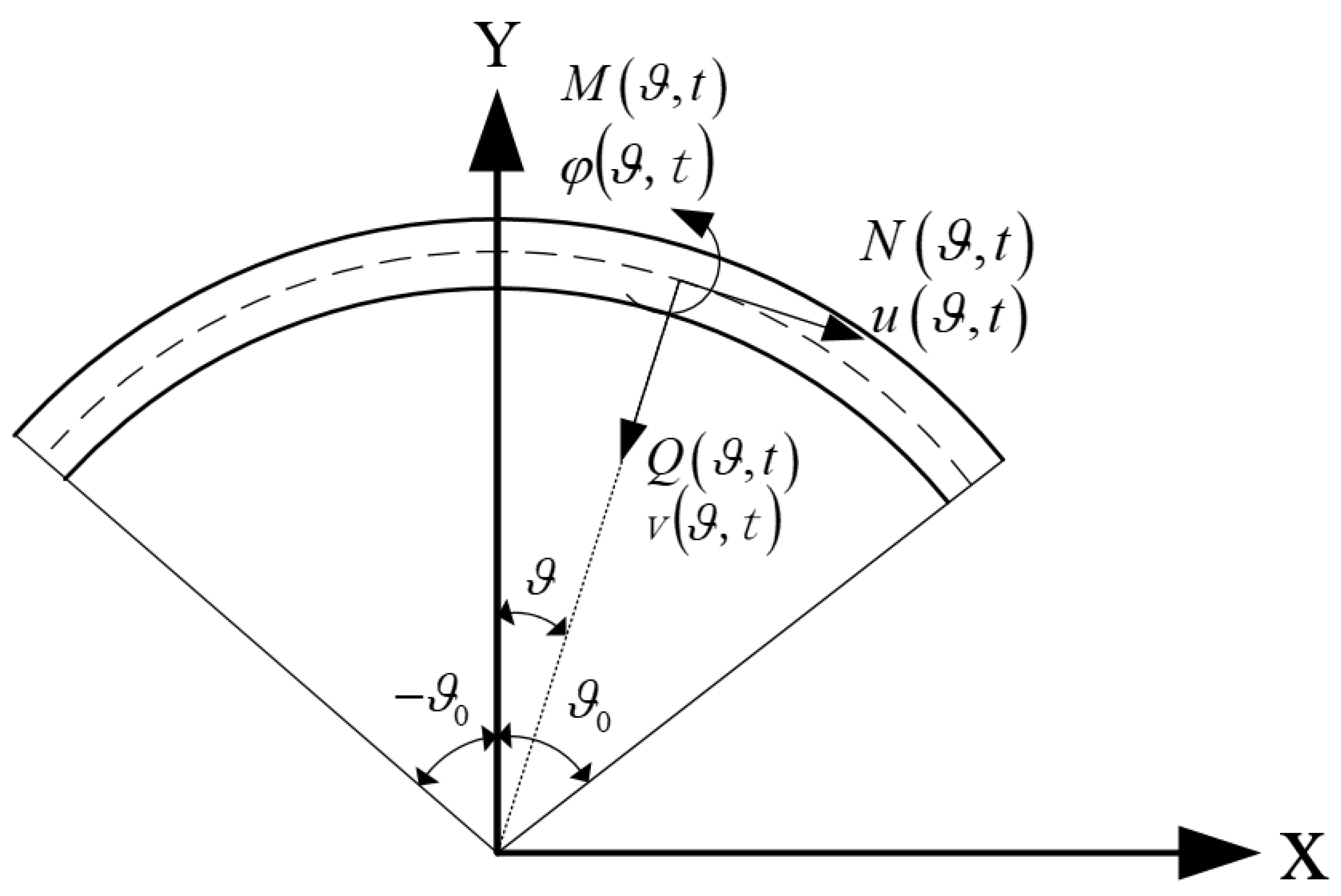
2. Model of the Arch and Procedure of Deterministic Free-Vibration Equations

2.1. Establishment of Free-Vibration Equations

The model of the arch is shown in Figure 1. Only the elastic deformation and the in-plane vibration are considered in the model. The term ϑ denotes the central angle formed between the radius of any cross-section and the Y axis, which is positively oriented in the clockwise direction; ϑ∈[−ϑ₀,ϑ₀], where ϑ₀ is half of the central angle of the whole arch. R is the radius and u(ϑ,t), v(ϑ,t), and φ(ϑ,t) are the tangential displacement, radial displacement, and bending slope of the cross-section at a given central angle ϑ and arbitrary time t, respectively.

The kinematic equation can be written as follows [6]:

$$\left\{\begin{array}{c}\frac{1}{R}\frac{\partial N\left(\vartheta ,t\right)}{\partial \vartheta }-\frac{Q\left(\vartheta ,t\right)}{R}=\rho A\frac{{\partial }^{2}u\left(\vartheta ,t\right)}{\partial t^2}\\ \frac{1}{R}\frac{\partial Q\left(\vartheta ,t\right)}{\partial \vartheta }+\frac{N\left(\vartheta ,t\right)}{R}=\rho A\frac{{\partial }^{2}v\left(\vartheta ,t\right)}{\partial t^2}\\ \frac{1}{R}\frac{\partial \mathit{M}\left(\vartheta ,t\right)}{\partial \vartheta }-Q\left(\vartheta ,t\right)=\rho I\frac{{\partial }^2\phi \left(\vartheta ,t\right)}{\partial t^2}\end{array}\right.$$

(1)

where ρ is the mass density for unit volume; A and I are the area and moment of inertia of the cross-section, respectively. N(ϑ,t), Q(ϑ,t), and M(ϑ,t) represent the axial force, shear force, and bending moment, respectively, and these internal forces can also be expressed by the constitutive relation of displacement as:

$$\left\{\begin{array}{c}N\left(\vartheta ,t\right)=\frac{EA}{R}\left(\frac{\partial u\left(\vartheta ,t\right)}{\partial \vartheta }-v\left(\vartheta ,t\right)\right)\\ Q\left(\vartheta ,t\right)=\frac{GA}{R{\kappa }_0}\left(u\left(\vartheta ,t\right)+\frac{\partial v\left(\vartheta ,t\right)}{\partial \vartheta }+R\phi \left(\vartheta ,t\right)\right)\\ M\left(\vartheta ,t\right)=\frac{EI}{R}\frac{\partial \phi \left(\vartheta ,t\right)}{\partial \vartheta }\end{array}\right.$$

(2)

in which E is Young’s modulus and G is shear modulus; κ₀ is the shear factor. Substituting the relations in (2) into Equation (1), and with u(ϑ,t), v(ϑ,t), and φ(ϑ,t) indicated as u, v, and φ, the equations can be expressed as follows:

$$\left\{\begin{array}{c}\frac{EA}{R^2}\frac{{\partial }^{2}u}{\partial {\vartheta }^2}-\frac{GA}{R^2{\kappa }_0}u-\left(\frac{EA}{R^2}+\frac{GA}{R^2{\kappa }_0}\right)\frac{\partial v}{\partial \vartheta }-\frac{GA}{R{\kappa }_0}\phi =\rho A\frac{{\partial }^{2}u}{\partial t^2}\\ \left(\frac{EA}{R^2}+\frac{GA}{R^2{\kappa }_0}\right)\frac{\partial u}{\partial \vartheta }+\frac{GA}{R^2{\kappa }_0}\frac{{\partial }^{2}v}{\partial {\vartheta }^2}-\frac{EA}{R^2}v+\frac{GA}{R{\kappa }_0}\frac{\partial \phi }{\partial \vartheta }=\rho A\frac{{\partial }^{2}v}{\partial t^2}\\ -\frac{GA}{R{\kappa }_0}u-\frac{GA}{R{\kappa }_0}\frac{\partial v}{\partial \vartheta }+\frac{EI}{R^2}\frac{{\partial }^2\phi }{\partial {\vartheta }^2}-\frac{GA}{{\kappa }_0}\phi =\rho I\frac{{\partial }^2\phi }{\partial t^2}\end{array}\right.$$

(3)

Equation (3) comprises the in-plan free-vibration equations. In general, the separation of variables can be employed to seek solutions that exhibit temporal harmony with frequency ω, so the displacement can be expressed as:

$$\left\{\begin{array}{c}u\left(\vartheta ,t\right)=U\left(\vartheta \right)\sin \left(\omega t\right)\\ v\left(\vartheta ,t\right)=V\left(\vartheta \right)\sin \left(\omega t\right)\\ \phi \left(\vartheta ,t\right)=\Phi \left(\vartheta \right)\sin \left(\omega t\right)\end{array}\right.$$

(4)

U(ϑ), V(ϑ), and Φ(ϑ) are indicated as U, V, and Φ, which represent the tangential, radial, and rotational vibration amplitude values of the structure, respectively. Substituting the relations in (4) into Equation (3), we obtain:

$$\left\{\begin{array}{c}\frac{EA}{R^2}\frac{d^{2}U}{d{\vartheta }^2}-\frac{GA}{R^2{\kappa }_0}U-\left(\frac{EA}{R^2}+\frac{GA}{R^2{\kappa }_0}\right)\frac{dV}{d\vartheta }-\frac{GA}{R{\kappa }_0}\Phi =-{\omega }^2\rho AU\\ \left(\frac{EA}{R^2}+\frac{GA}{R^2{\kappa }_0}\right)\frac{dU}{d\vartheta }+\frac{GA}{R^2{\kappa }_0}\frac{d^{2}V}{d{\vartheta }^2}-\frac{EA}{R^2}V+\frac{GA}{R{\kappa }_0}\frac{d\Phi }{d\vartheta }=-{\omega }^2\rho AV\\ -\frac{GA}{R{\kappa }_0}U-\frac{GA}{R{\kappa }_0}\frac{dV}{d\vartheta }+\frac{EI}{R^2}\frac{d^2\Phi }{d{\vartheta }^2}-\frac{GA}{{\kappa }_0}\Phi =-{\omega }^2\rho I\Phi \end{array}\right.$$

(5)

The equations describing the boundary conditions are written as follows:

Clamped edge boundary U = 0, V = 0, Φ = 0 at ϑ = ±ϑ₀

(6)

2.2. Establishment of Free-Vibration Equations

In this subsection, our primary objective is to derive a solution for the system of ordinary differential equations. Directly integrating the equations incurs significant complexity, thus necessitating the discovery of a concise and efficient approach. The differential quadrature (DQ) method is a highly effective approach for solving partial and ordinary differential equations. Its fundamental principle involves partitioning the domain of independent variables for smooth functions into discrete sample points according to specific rules and approximating the derivative of the function with respect to these independent variables as a weighted sum of their corresponding function values [11,12,13]. Therefore, the nth order derivative of function f(ϑ) with respect to ϑ at the ith point ϑ_i is approximated as follows:

$${\left.\frac{{\partial }^{n}f\left(\vartheta \right)}{\partial {\vartheta }^n}\right|}_{\vartheta ={\vartheta }_i}={\displaystyle \sum _{j=1}^H{\xi }_{ij}^{\left(n\right)}f\left({\vartheta }_j\right)},i=1,2,\dots ,H$$

(7)

where ${\xi }_{ij}^{\left(n\right)}$ denotes the nth-order derivative weighting coefficients of ϑ at the ith sample point calculated for the jth sample points in the domain, H is the total number of sample points, and f(ϑ_i) is the function value at point ϑ_i. The weighting coefficients can be determined by Lagrange polynomial functions, and the first-order derivative weighting coefficients are:

$${\xi }_{ij}^{\left(1\right)}=\frac{L^{\left(1\right)}\left({\vartheta }_i\right)}{\left({\vartheta }_i-{\vartheta }_j\right)L^{\left(1\right)}\left({\vartheta }_j\right)},i,j=1,2,\dots ,H,i\ne j$$

where $L^{\left(1\right)}\left({\vartheta }_j\right)={\displaystyle \prod _{i=1,i\ne j}^H\left({\vartheta }_j-{\vartheta }_i\right)}$.

$${\xi }_{ii}^{\left(1\right)}=-{\displaystyle \sum _{j=1,j\ne i}^H{\xi }_{ij}^{\left(1\right)}},i,j=1,2,\dots ,H$$

(8)

The second- and higher-order derivative weighting coefficients are:

$$\begin{gathered} {\xi }_{ij}^{\left(n\right)}=n\left({\xi }_{ii}^{\left(n-1\right)}{\xi }_{ij}^{\left(1\right)}-\frac{{\xi }_{ij}^{\left(n-1\right)}}{{\vartheta }_i-{\vartheta }_j}\right),i,j=1,2,\dots ,H,i\ne j,n=2,3,\dots ,H-1 \\ {\xi }_{ii}^{\left(n\right)}=-{\displaystyle \sum _{j=1,j\ne i}^H{\xi }_{ij}^{\left(n\right)}},i,j=1,2,\dots ,H,n=2,3,\dots ,H-1 \end{gathered}$$

(9)

Each order of the derivative weighting coefficients can be obtained according to the above formulas. It is evident that the computation of derivative weight coefficients beyond the second order necessitates prior acquisition of first-order weight coefficients. The selection of appropriate sample points serves as a fundamental basis for ensuring both accuracy and efficiency in DQ method calculations. The Chebyshev–Gauss–Lobatto (C-G-L) grid distribution [11] is employed in this paper. According to the C-G-L rule, the sample point r_i on the standard interval [0,1] is expressed as:

$$r_i=\frac{1-\cos \left(\frac{i-1}{H-1}\pi \right)}{2},i=1,2,\dots ,H$$

(10)

and its values can be established by mapping the relationship with ϑ_i as follows:

$${\vartheta }_i=-{\vartheta }_0+r_i\cdot 2{\vartheta }_0,i=1,2,\dots ,H$$

(11)

The required sample points for this method are now available. After selecting a specific number of sample points based on the calculation requirements, the derivative weighting coefficient can be obtained through relations (8) and (9).

Using the DQ method, the arch is discretized according to sample points ϑ_i, and the propositions of the original Equation (5) can be rewritten as:

$$\left\{\begin{array}{c}\frac{EA}{R^2}{\displaystyle \sum _{j=1}^H{\xi }_{ij}^{\left(2\right)}}{U}_j-\frac{GA}{R^2{\kappa }_0}{U}_i-\left(\frac{EA}{R^2}+\frac{GA}{R^2{\kappa }_0}\right){\displaystyle \sum _{j=1}^H{\xi }_{ij}^{\left(1\right)}{V}_j}-\frac{GA}{R{\kappa }_0}{\Phi }_i=-{\omega }^2\rho A{U}_i\\ \left(\frac{EA}{R^2}+\frac{GA}{R^2{\kappa }_0}\right){\displaystyle \sum _{j=1}^H{\xi }_{ij}^{\left(1\right)}{U}_j}+\frac{GA}{R^2{\kappa }_0}{\displaystyle \sum _{j=1}^H{\xi }_{ij}^{\left(2\right)}}{V}_j-\frac{EA}{R^2}{V}_i+\frac{GA}{R{\kappa }_0}{\displaystyle \sum _{j=1}^H{\xi }_{ij}^{\left(1\right)}{\Phi }_j}=-{\omega }^2\rho A{V}_i\\ -\frac{GA}{R{\kappa }_0}{U}_i-\frac{GA}{R{\kappa }_0}{\displaystyle \sum _{j=1}^H{\xi }_{ij}^{\left(1\right)}{V}_j}+\frac{EI}{R^2}{\displaystyle \sum _{j=1}^H{\xi }_{ij}^{\left(2\right)}{\Phi }_j}-\frac{GA}{{\kappa }_0}{\Phi }_i=-{\omega }^2\rho I{\Phi }_i\end{array}\right.$$

(12)

where U_i, V_i, and Φ_i represent the tangential, radial, and rotational vibration amplitude values, respectively, at θ_i, i = 1, 2,…H. The set of equations can be reduced to

$$\left[\mathit{K}\right]\left\{\mathit{\delta }\right\}+{\omega }^2\left[\mathit{M}\right]\left\{\mathit{\delta }\right\}=0$$

(13)

in which [K] and [M] are the global stiffness matrix and mass matrix, respectively, and {δ} = {U₁ V₁ Φ₁…U_H V_H Φ_H} is the generalized displacement vector. Relation (6) can be transformed into:

U_i = 0, V_i = 0, Φ_i = 0, i = 1, H

(14)

Considering the boundary condition, Equation (13) can be written as

$$\left[\begin{array}{cc}\left[{\mathit{K}}_{bb}\right]& \left[{\mathit{K}}_{bd}\right]\\ \left[{\mathit{K}}_{db}\right]& \left[{\mathit{K}}_{dd}\right]\end{array}\right]\left\{\begin{array}{c}\left\{{\mathit{\delta }}_b\right\}\\ \left\{{\mathit{\delta }}_d\right\}\end{array}\right\}+{\omega }^2\left[\begin{array}{cc}\left[\mathbf{0}\right]& \left[\mathbf{0}\right]\\ \left[\mathbf{0}\right]& \left[{\mathit{M}}_{dd}\right]\end{array}\right]\left\{\begin{array}{c}\left\{{\mathit{\delta }}_b\right\}\\ \left\{{\mathit{\delta }}_d\right\}\end{array}\right\}=0$$

(15)

The subscripts ‘b’ and ‘d’ in the matrix denote the components related to the boundary and internal domain, respectively, in Equation (15). The preservation of only the internal domain displacement vector is employed to streamline computation and enhance efficiency. Now Equation (15) can be expressed as follows:

$$\left(\left[{\mathit{K}}_{dd}\right]-\left[{\mathit{K}}_{db}\right]{\left[{\mathit{K}}_{bb}\right]}^{-1}\left[{\mathit{K}}_{bd}\right]\right)\left\{{\mathit{\delta }}_d\right\}+{\omega }^2\left[{\mathit{M}}_{dd}\right]\left\{{\mathit{\delta }}_d\right\}=0$$

(16)

Letting $\left[\stackrel{⌢}{\mathit{K}}\right]=\left[{\mathit{K}}_{dd}\right]-\left[{\mathit{K}}_{db}\right]{\left[{\mathit{K}}_{bb}\right]}^{-1}\left[{\mathit{K}}_{bd}\right]$, $\left[\stackrel{⌢}{\mathit{M}}\right]=\left[{\mathit{M}}_{dd}\right]$, Equation (16) can be written as:

$$\left[\stackrel{⌢}{\mathit{K}}\right]\left\{{\mathit{\delta }}_d\right\}+{\omega }^2\left[\stackrel{⌢}{\mathit{M}}\right]\left\{{\mathit{\delta }}_d\right\}=0$$

(17)

The natural frequencies can be obtained by the eigenvalue decomposition of Equation (17).

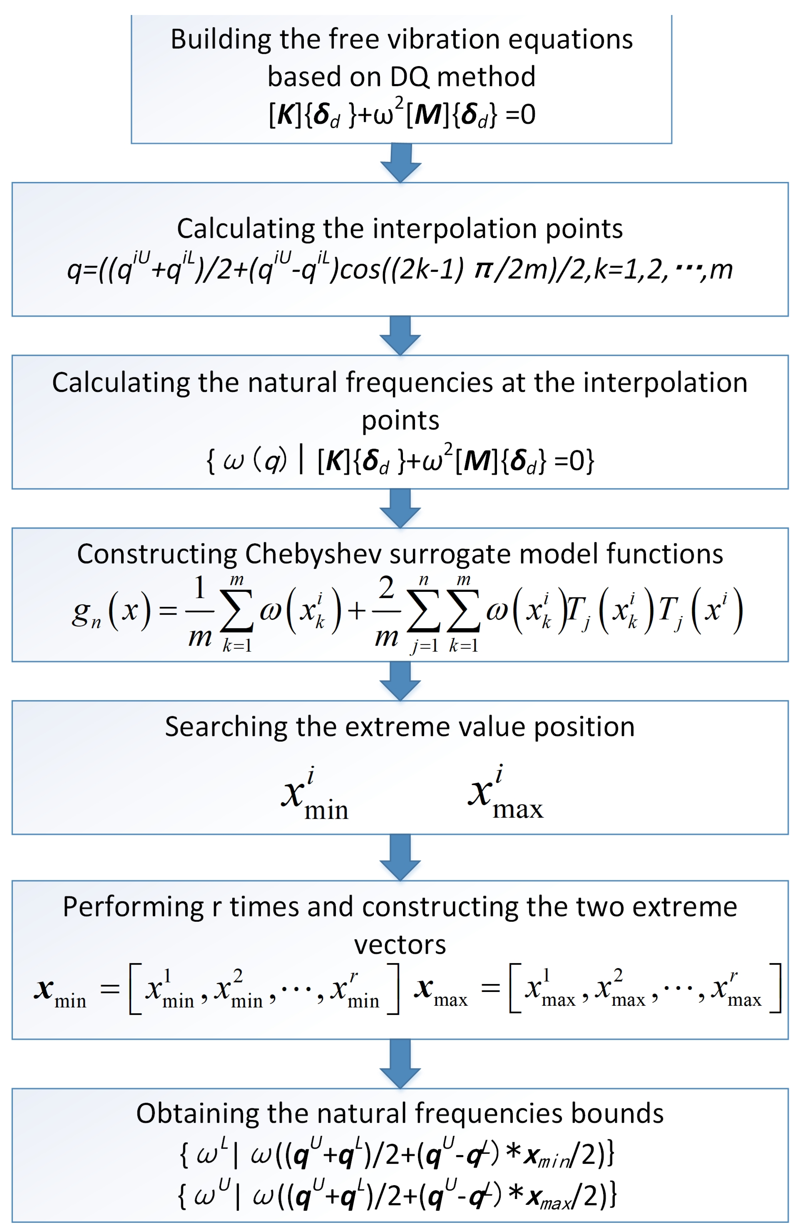
3. General Polynomial Surrogate Model for Interval Natural Frequency Analysis

In this section, the uncertain natural frequency bounds of an arch will be analyzed with Chebyshev interval algorithms. It has been demonstrated that for a continuous function f(x) defined in [a, b], there always exists a polynomial g(x) that approximates it with an error no larger than an arbitrary small positive quantity ε. On this basis, the Chebyshev polynomial surrogate (CPS) model is utilized to deal with uncertain dynamic problems; the frequencies are treated as the proposed function f(x) and can be approximated by orthogonal polynomials with acceptable errors in the following. The original dynamic questions can be modeled as simple mathematical functions by using a few interpolation points, which can save the computational cost of the traditional Monte Carlo simulation (MCS) without losing accuracy. As mentioned previously, the geometric dimensions of the cross-sectional area and physical parameters such as the Young’s modulus may be uncertain. Due to the lack of necessary information, it is a complicated task to model the uncertainties probabilistically. However, only their bounds are needed in the interval approach, which can be achieved easily. Therefore, it is more reasonable to regard the uncertainties as interval variables. An uncertain parameter is regarded as an interval parameter q^I, where superscript I denotes the interval variable, and can be denoted as:

$$q^I=\left[q^L,q^U\right]=\left\{q\in R\left|q^L\le q\le q^U\right.\right\}=\left[q^C-\beta q^C\le q\le q^C+\beta q^C\right]$$

(18)

in which q^L, q^U, and q^C denote the lower bound, upper bound, and nominal value of the interval parameter q^I, respectively. Deviation degree β denotes the deviation coefficients. R is the set of all real numbers. If there is more than one uncertain parameter, the expression above can be expressed in the form of multi-dimensional interval vectors, as:

$${\mathit{q}}^I=\left[{\mathit{q}}^L,{\mathit{q}}^U\right]=\left\{{\mathit{q}}^L\le \mathit{q}\le {\mathit{q}}^U\right\}=\left\{q_i\in R\left|q_i^L\le q_i\le q_i^U\right.\right\}$$

(19)

q^I is the uncertain parameters vector, where i = 1, 2,…r. r is the total number of uncertain parameters, and the parameters are assumed to be mutually independent in the following. Considering the matrices in the free-vibration equations for the uncertain arches as the function of the uncertain parameter, Equation (17) can be rewritten in the interval form

$$\left[\stackrel{⌢}{\mathit{K}}\left({\mathit{q}}^I\right)\right]\left\{{\mathit{\delta }}_d\left({\mathit{q}}^I,\vartheta \right)\right\}+\omega {\left({\mathit{q}}^I\right)}^2\left[\stackrel{⌢}{\mathit{M}}\left({\mathit{q}}^I\right)\right]\left\{{\mathit{\delta }}_d\left({\mathit{q}}^I,\vartheta \right)\right\}=0$$

(20)

The goal of this study is to determine the interval range of natural frequencies, and a surrogate model based on Chebyshev orthogonal polynomial approximation theory is introduced to achieve this. First, the one-dimensional uncertain model is analyzed. The first type of Chebyshev orthogonal polynomial is T_n(x) = cos(narccosx), x ∈ [−1,1], where n is an arbitrary positive integer. T_n(x) is orthogonal on [−1,1] with respect to the weight function ρ(x) = (1 − x²)^1/2, and its recurrence formulas are as follows:

$$\left\{\begin{array}{c}{T}_0\left(x\right)=1\\ T_1\left(x\right)=x\\ T_{n+1}\left(x\right)=2x{T}_n\left(x\right)-T_{n-1}\left(x\right)\end{array}\right.,n=1,2,\dots$$

(21)

The one-dimensional n-order Chebyshev polynomial approximation of function f(x) is formulated as:

$$f\left(x\right)\approx g_n\left(x\right)=\frac{a_0}{2}+{\displaystyle \sum _{i=1}^n{a}_i{T}_i\left(x\right)},x\in \left[-1,1\right]$$

(22)

in which a_i is the expansion coefficient and

$$a_i=\frac{2}{\pi }{\displaystyle {\int }_{-1}^1\frac{\tilde{f}\left(x\right)T_i\left(x\right)}{\sqrt{1-x^2}}dx}, i = 0,1,2,\dots ,n$$

(23)

where $\tilde{f}\left(x\right)$ is the deterministic value of f(x) and n is the expansion order. In general, the direct integration of a_i poses significant complexities. However, when compared to this approach, employing the Gauss–Chebyshev integration formula proves to be a more efficient and expeditious method for obtaining a_i. The Gauss–Chebyshev integration formula is a type of interpolation integral formula expressed as follows:

$${\displaystyle {\int }_a^b\rho \left(x\right)p\left(x\right)}dx={\displaystyle \sum _{k=1}^m{A}_{k}p\left(x_k\right)}$$

(24)

in which m is the number of integral points and should satisfy m ≥ n + 1.

In the Gauss–Chebyshev integration, the interpolation points involved in the integration process are the zeros of m-degree Chebyshev polynomials, which are given by:

$$x_k=\cos \left(\frac{2k-1}{2m}\pi \right),k=1,2,\dots ,m$$

(25)

For Equation (24), the weight function (1 − x²)^1/2 of the Chebyshev orthogonal polynomial is chosen as ρ(x), and in this case, all the integral coefficients A_k = π/m [27]. Substituting this into Equation (24), the expansion coefficient a_i can be expressed as

$$a_i=\frac{2}{\pi }{\displaystyle {\int }_{-1}^1\frac{f\left(x\right)T_i\left(x\right)}{\sqrt{1-x^2}}}dx\approx \frac{2}{\pi }\frac{\pi }{m}{\displaystyle \sum _{k=1}^{m}f\left(x_k\right)}T\left(x_k\right)=\frac{2}{m}{\displaystyle \sum _{k=1}^{m}f\left(x_k\right)}T\left(x_k\right)$$

(26)

Substituting this into Equation (22), we obtain

$$g_n\left(x\right)=\frac{1}{m}{\displaystyle \sum _{k=1}^{m}f\left(x_k\right)}+\frac{2}{m}{\displaystyle \sum _{i=1}^n{\displaystyle \sum _{k=1}^{m}f\left(x_k\right)T_i\left(x_k\right)T_i\left(x\right)}}$$

(27)

Now the polynomial surrogate model function based on Chebyshev orthogonal polynomials can be constructed. It is evident that once the original frequency values at interpolation points, as given by Equation (25), are obtained from the deterministic model in Equation (17), the expansion coefficient a_i can be calculated immediately, thereby simultaneously obtaining the surrogate-model function. The upper and lower bounds of the function being approximated can be obtained by searching the maximum and minimum values of g_n(x) on standard interval [−1,1], which can be easily achieved based on the maximum theorem of a continuous function on closed intervals. Moreover, linear transformation does not change the relative locations of the extreme values. Considering the arbitrary interval distribution of the uncertain parameter x, and the fact that the Chebyshev polynomial surrogate model is applicable only for the standard interval [−1,1], it is necessary to transfer the parameter to a standard interval:

$$x_i=\frac{2q_i-\left(q^U+q^L\right)}{q^U-q^L}, q_i\in \left[q^L,q^U\right]$$

(28)

The roots of the derivative equation are:

$$\left\{x_r\left|g_n^{\prime }\left(x\right)=0\right.\right\}$$

(29)

The extremal value points x_min and x_max, which correspond to the uncertain parameter x, are determined by comparing the values of g_n(x_r), g_n(−1), and g_n(1). This implies that the natural frequencies attain their maximum and minimum values at these points. The corresponding locations of x will be marked as x_min and x_max.

Supposing that multiple uncertain parameters are independent, for r-dimensional uncertain parameter vector q^I, the process of searching the extremum should be performed r times to obtain the maximum and minimum frequency value locations for each parameter. Two extremum vectors will be obtained:

$$\left\{\begin{array}{c}{\mathit{x}}_{\min }=\left[x_{1,\min },x_{2,\min },\cdots ,x_{r,\min }\right]\\ {\mathit{x}}_{\max }=\left[x_{1,\max },x_{2,\max },\cdots ,x_{r,\max }\right]\end{array}\right.$$

(30)

Accordingly, the two deterministic parameter vectors that account for the bounds of the frequencies will be defined as follows:

$$\left\{\begin{array}{c}{\mathit{q}}_{\min }={\mathit{q}}^C+\left({\mathit{q}}^U-{\mathit{q}}^L\right){\mathit{x}}_{\min }\\ {\mathit{q}}_{\max }={\mathit{q}}^C+\left({\mathit{q}}^U-{\mathit{q}}^L\right){\mathit{x}}_{\max }\end{array}\right.$$

(31)

where q^C, q^U, and q^L represent the nominal values, upper bounds, and lower bounds of the uncertain parameters, respectively, which are all deterministic. Substituting Equation (31) into Equation (17), the natural-frequency bounds can be obtained from two differential equations:

$$\left\{\begin{array}{c}\left[\stackrel{⌢}{\mathit{K}}\left({\mathit{q}}_{\min }\right)\right]\left\{{\mathit{\delta }}_d\left({\mathit{q}}_{\min },\vartheta \right)\right\}+\mathit{\omega }{\left({\mathit{q}}_{\min }\right)}^2\left[\stackrel{⌢}{\mathit{M}}\left({\mathit{q}}_{\min }\right)\right]\left\{{\mathit{\delta }}_d\left({\mathit{q}}_{\min },\vartheta \right)\right\}=0\\ \left[\stackrel{⌢}{\mathit{K}}\left({\mathit{q}}_{\max }\right)\right]\left\{{\mathit{\delta }}_d\left({\mathit{q}}_{\max },\vartheta \right)\right\}+\mathit{\omega }{\left({\mathit{q}}_{\max }\right)}^2\left[\stackrel{⌢}{\mathit{M}}\left({\mathit{q}}_{\max }\right)\right]\left\{{\mathit{\delta }}_d\left({\mathit{q}}_{\max },\vartheta \right)\right\}=0\end{array}\right.$$

(32)

The solutions to Equation (32) are all deterministic and of the same size as the original equation denoted by Equation (17), and the equations can be solved easily. The whole computational procedure of the natural frequency bounds obtained using the CPS model is illustrated in Figure 2.

4. Numerical Simulation and Discussion

In this section, a circular arch with interval uncertainties will be simulated numerically. The first fourth-order deterministic natural frequencies are presented in the first subsection with the deterministic parameters, using the DQ method. Then, the accuracy and efficiency of the proposed CPS model in computing the natural frequencies are validated by comparison with the MCS in the second subsection. In the third subsection, different uncertain parameters such as the cross-sectional height and Young’s modulus are considered, and the corresponding bounds of the natural frequencies are shown. The numerical simulations are conducted using the MATLAB R2014a software.

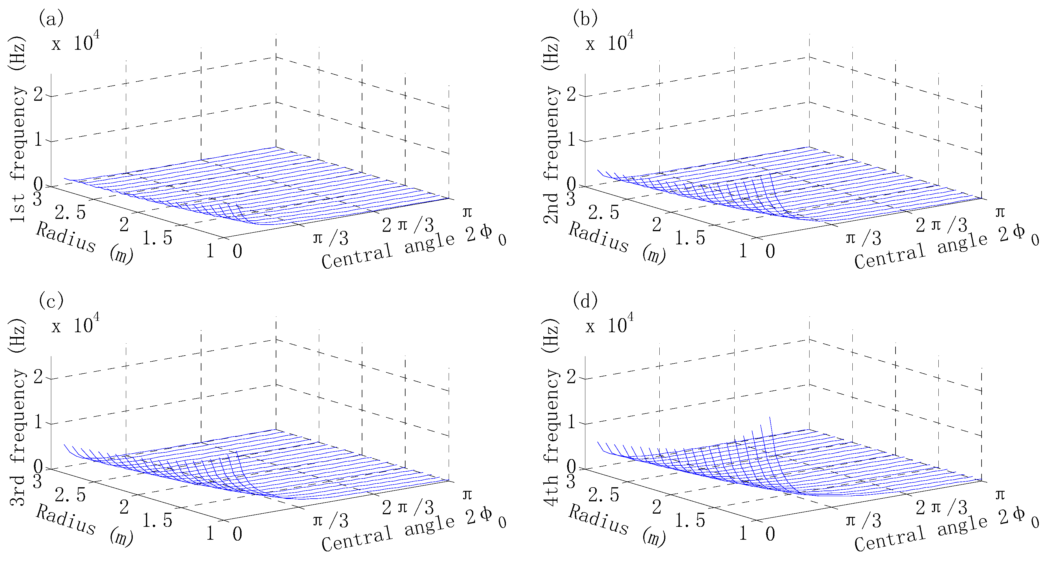
4.1. The Natural Frequencies Based on the Traditional Deterministic Method

According to the calculation example provided in reference [19], the arch cross-section is assumed to be rectangular; its physical parameters are presented in

Table 1. Geometrical and physical parameters of arch.

Description	Value
Cross-sectional width b	0.06 m
Cross-sectional height h	0.08 m
Density of mass ρ	7860 kg/m3
Young’s modulus E	2.1 × 1011 pa
Poisson’s coefficient ν	0.3
Shear factor κ0	1.2

. In this paper, the total number of discretized sample points of arch H is 21. Waterfall plots of the first fourth-order natural frequencies with the central angle varying in the interval [π/6, π] and the radius varying in the interval [1,3] are shown in Figure 3. Firstly, it is shown that, under the conditions of equal radius and central angle, the natural frequency demonstrates a discernible upward trend with increasing orders, which aligns convincingly with empirical evidence. Then, it is also shown that the frequency of each order increases as the radius and central angle decrease, with a more pronounced increase observed in higher-order frequencies compared to lower-order frequencies. Furthermore, the frequency remains numerically continuous within the range of the central angle, thus confirming the appropriateness of the surrogate model utilized in this paper. Specifically, it is essential for the objective function of the model to maintain continuity.

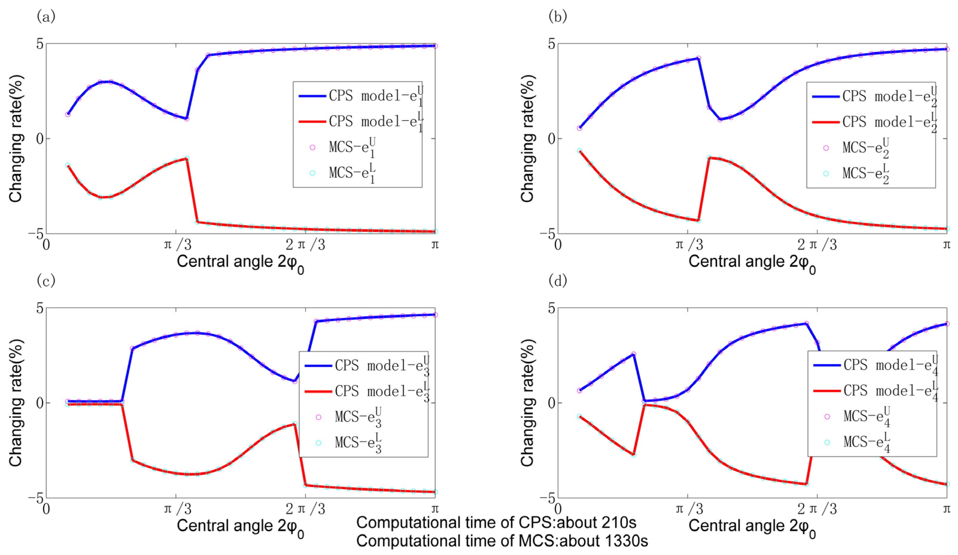
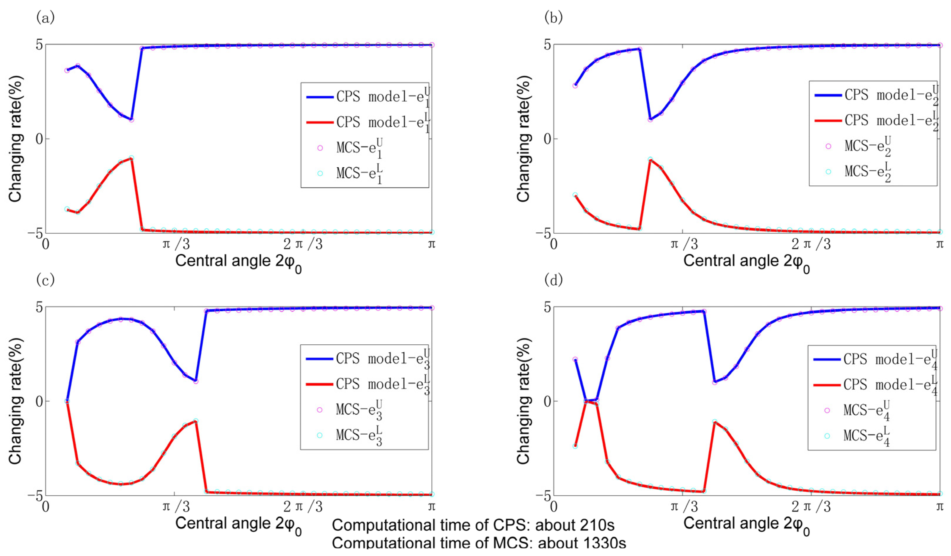
4.2. Comparisons of CPS Model with MCS in Calculating Natural Frequencies

In order to assess the accuracy and efficiency of the CPS model in estimating an uncertain natural frequency, the MCS will be used for comparison. A sufficient number of samples is the guarantor ensuring the accuracy of the simulation in the MCS, and 500 samples are utilized in this MCS. The expansion order n of the CPS model takes the value 3 and the number of the integral point m takes the value 5. Variables ${\omega }_i^U$ and ${\omega }_i^L$ represent the upper bound and lower bound of the ith natural frequency, respectively. Variables $e_i^U$ and $e_i^L$ represent the upper bound and lower bound of the ith frequency changing rate, respectively, which can be regarded as an indication of the fluctuation in natural frequency and can be formulated as

$$\left\{\begin{array}{c}{e}_i^U=\frac{{\omega }_i^U-{\omega }_i}{{\omega }_i}\times 100\%\\ e_i^L=\frac{{\omega }_i^L-{\omega }_i}{{\omega }_i}\times 100\%\end{array}\right.$$

(33)

Accounting for inevitable manufacturing tolerances, the cross-sectional height is considered as an uncertainty parameter, with a deviation degree of 5%. The radius takes values of 1 m and 3 m, while the central angle still varies in the interval [π/6, π] for legibility. Figure 4 and Figure 5 show the comparisons of changing rates of the first fourth-order uncertain natural frequencies. It is shown that the results obtained from both models exhibit excellent agreement in terms of the changing rate for each order’s frequencies, thereby formalizing the accuracy of the proposed interval model and its applicability in determining frequency intervals. Furthermore, the CPS model demonstrates a computational time that is approximately 85% shorter than that of MCS, thus confirming its high efficiency. Additionally, it is observed that when maintaining an equal radius, there exist fluctuation characteristics and a minimum value in the relationship between the changing rate and central angle. Moreover, as the radius increases, the position of the minimum value shifts towards the left along the horizontal axis representing the central angle.

4.3. Uncertain Natural Frequency Investigations Considering Different Uncertain Parameters

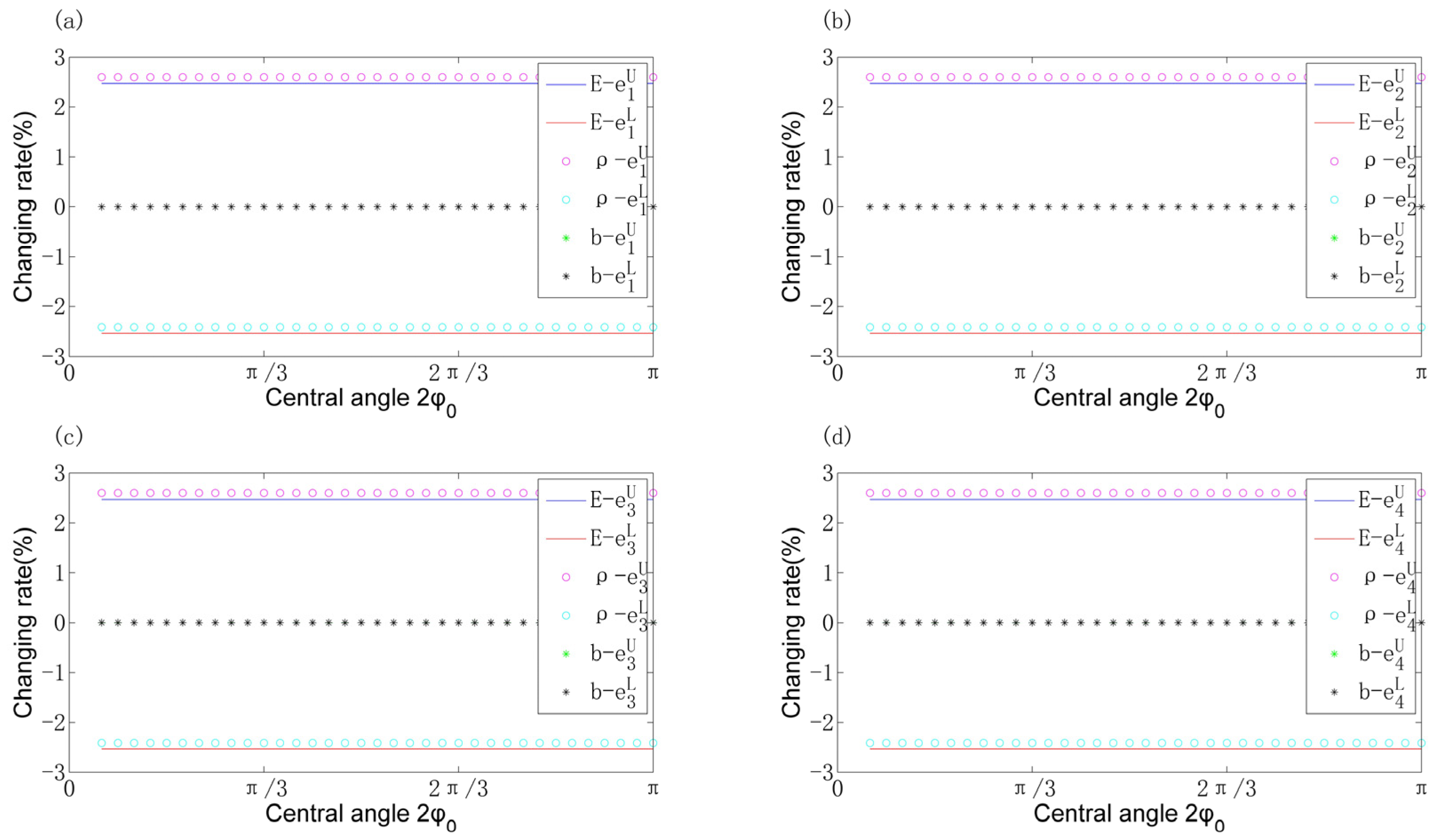
4.3.1. Single Uncertain Parameter

In the first part of this subsection, a single uncertain parameter is considered. Parts of the numerical simulation results are illustrated regarding the effect of the uncertain cross-sectional height in the comparative analysis previously presented, and here the width of the cross-section is considered with the same deviation degree. Taking into consideration material dispersion, Young’s modulus and the density of mass are regarded as uncertain parameters, with respective deviation degrees of 5%. The simulation results are shown in Figure 6. It is found that the bounds of the changing rate are drawn as straight lines in the presence of each of the uncertainties above, and further investigations demonstrate that these phenomena remain unaffected by variations in radius. Furthermore, the natural frequencies are minimally influenced by the uncertain width of the cross-section; however, they exhibit greater sensitivity to variations in the uncertain cross-sectional height compared with Young’s modulus and the density of mass. It can be seen that the physical parameters, including Young’s modulus and the density of mass, demonstrate a linear relationship with the natural frequencies through eigenvalue decomposition of the free-vibration equation. Additionally, the cross-sectional width can be canceled on both sides of the equation. Moreover, a nonlinear correlation exists between the cross-sectional height and the moment of inertia, subsequently affecting the natural frequency. This observation elucidates the distinct influences of each parameter on the uncertain dynamic characteristics.

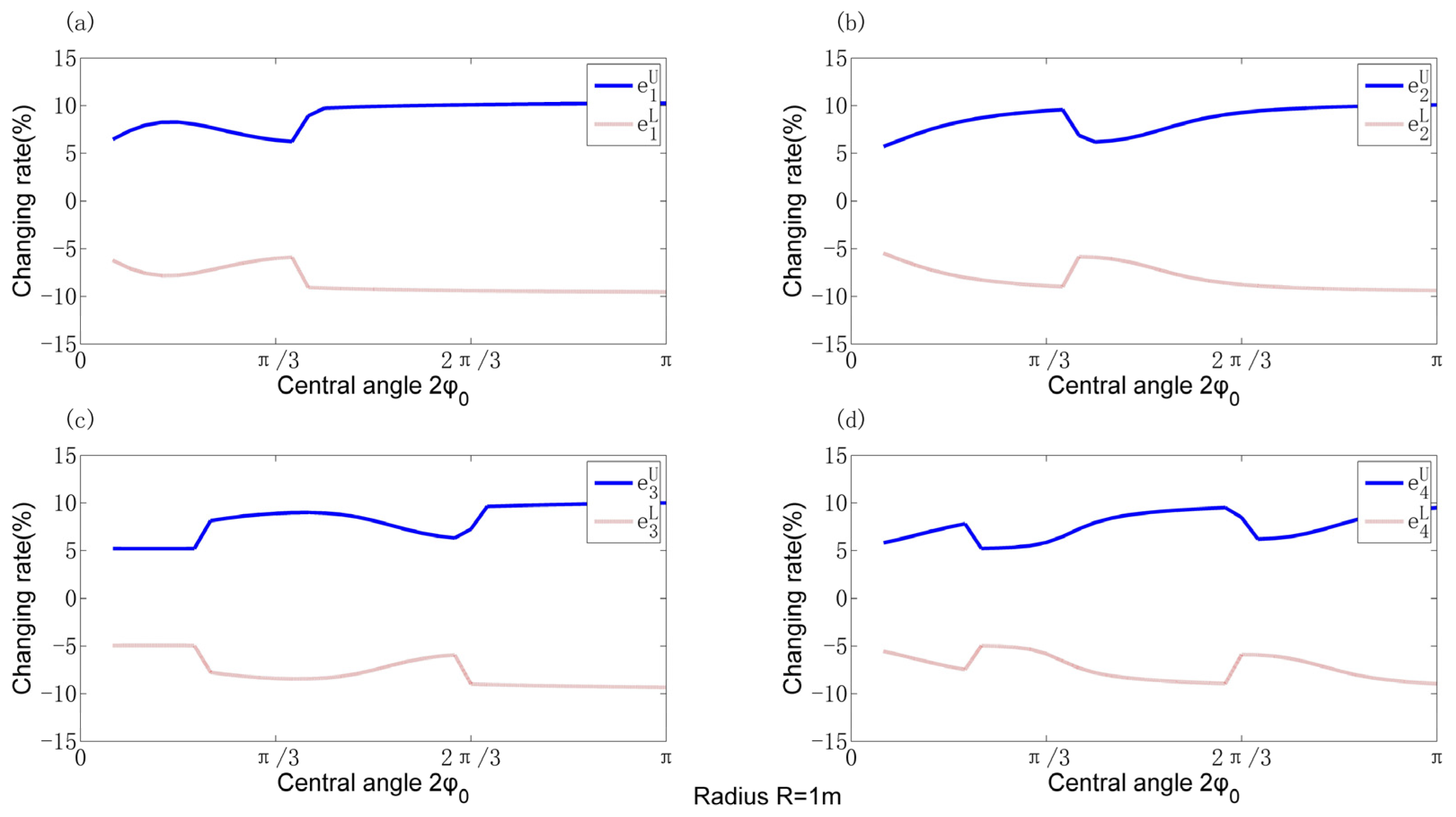
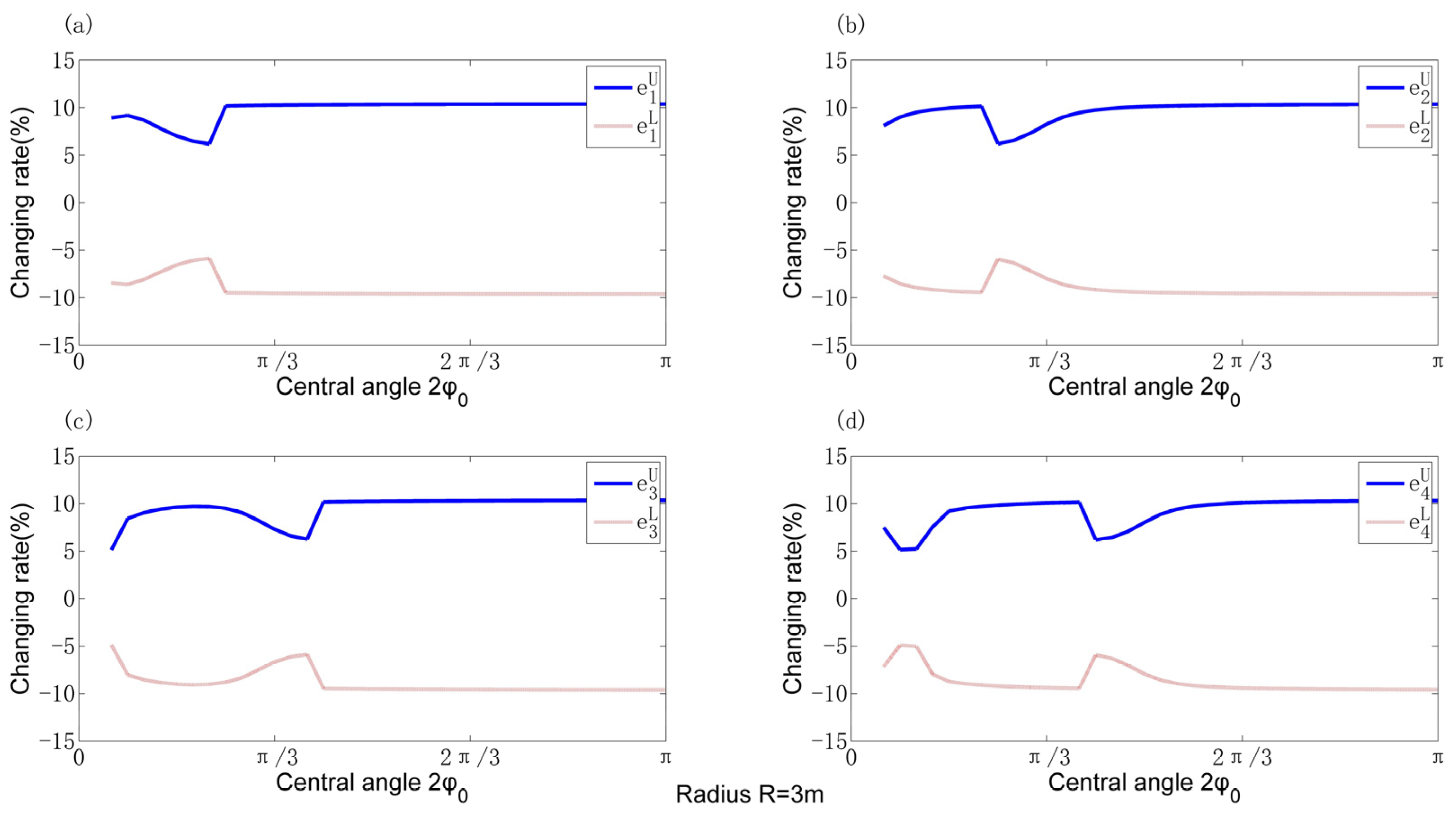
4.3.2. Multiple Uncertain Parameters

In order to investigate the characteristics of frequency under the influence of multiple uncertain parameters, all the aforementioned uncertainties are considered simultaneously. However, employing the MCS requires a substantial number of samples for each parameter in order to ensure accuracy, resulting in unacceptable computational costs. Utilizing the CPS model can significantly reduce these costs and provide notable efficiency advantages. The numerical simulation results depicting multi-dimensional uncertainty are presented in Figure 7 and Figure 8. The changing rates of frequencies surpass those observed when considering individual parameters separately, indicating a linear superposition of the effects of all uncertainties. Furthermore, although resembling single cross-sectional height considerations in terms of image shape, fluctuations exhibit smaller amplitudes. Additionally, as the radius increases, the phenomenon that the position of the minimum value shifts to the left along the horizontal axis representing the central angle does not change.

5. Conclusions

The linear natural frequencies of arches under interval-uncertain parameters were analyzed in this study. By coupling the DQ method and the Chebyshev approximation theory, a surrogate model was established to solve the uncertainty problem with respect to the dynamic characteristics of arches. The non-intrusive interval method is valid in free-vibration analysis, for which probabilistic methods cannot be utilized due to a lack of essential prior information. The accuracy and effectiveness of the proposed CPS model were demonstrated via a comparative study of the natural frequency ranges of the arch obtained using the MCS and the model. It is clear that the CPS model is more efficient, and this will be more obvious in multiple-uncertainty situations, because the sample points in multiple dimensions are enormous, while the interpolation numbers used in the CPS model remain acceptable. Based on the results of several cases exhibited in the foregoing sections, the following conclusions can be made:

• Some geometrical parameters, such as the cross-sectional height, were found to be sensitive, which will cause large fluctuations in the dynamic properties.
• The influence of most uncertain physical parameters on the natural frequencies exhibits a linear relationship which remains unaffected by variations in radius and central angle. However, different parameters yield distinct rates of change in frequency.
• In the case of multi-dimensional uncertainty, the changing rate of frequencies surpasses that of any individual parameter, as it represents a linear superposition of the combined influence exerted by each parameter.

The analysis method employed in this study is non-intrusive and convenient, and has been demonstrated to be an efficient approach for addressing the free-vibration problems of arches with uncertainties. It is widely accepted that, despite the uncertain parameters, there should be a linear relationship between the natural frequency of the linear elastic arch and the deviation degree of an uncertain parameter. However, this study has revealed intriguing variations in the influences of different parameters on the natural frequency, sometimes exhibiting elusive changes. The methodology employed can be extended to calculate both natural frequencies and dynamic responses for nonlinear arches in future studies, which is expected to yield more valuable insights.

References

1. Deraemaeker, A.; Worden, K. A comparison of linear approaches to filter out environmental effect in structural health monitoring. Mech. Syst. Signal Process. 2018, 105, 1–15. [Google Scholar] [CrossRef]
2. Haichen, S.; Keith, W.; Elizabeth, J.C. A regime-switching cointegration approach for removing environmental and operational variations in structural health monitoring. Mech. Syst. Signal Process. 2018, 103, 381–397. [Google Scholar]
3. Marco, C.; Giulia, C.; Luca, Z.F. System identification via Fast Relaxed Vector Fitting for the Structural Health Monitoring of masonry bridges. Structures 2021, 30, 277–293. [Google Scholar]
4. Maes, K.; Van Meerbeeck, L.; Reynders, E.P.B.; Lombaert, G. Validation of vibration-based structural health monitoring on retrofitted railway bridge KW51. Mech. Syst. Signal Process. 2022, 165, 108380. [Google Scholar] [CrossRef]
5. Doan, D.; Zenkour, A.; Thom, D. Finite element modeling of free vibration of cracked nanoplates with flexoelectric effects. Eur. Phys. J. Plus 2022, 137, 447. [Google Scholar] [CrossRef]
6. Van Do, T.; Hong Doan, D.; Chi Tho, N.; Dinh Duc, N. Thermal buckling analysis of cracked functionally graded plates. Int. J. Struct. Stab. Dyn. 2022, 22, 2250089. [Google Scholar] [CrossRef]
7. Ghemari, Z.; Belkhiri, S. Mechanical resonator sensor characteristics development for precise vibratory analysis. Sens. Imaging 2021, 22, 40. [Google Scholar] [CrossRef]
8. Ghemari, Z.; Saad, S.; Khettab, K. Improvement of the vibratory diagnostic method by evolution of the piezoelectric sensor performances. Int. J. Precis. Eng. Manuf. 2019, 20, 1361–1369. [Google Scholar] [CrossRef]
9. Ghemari, Z. Progression of the vibratory analysis technique by improving the piezoelectric sensor measurement accuracy. Microw. Opt. Technol. Lett. 2018, 60, 2972–2977. [Google Scholar] [CrossRef]
10. Ekrem, T.; Oznur, O. Exact solution of free in-plane vibration of a stepped circular arch. J. Sound Vib. 2006, 295, 725–738. [Google Scholar]
11. Erasmo, V.; Michele, D.; Francesco, T. Analytical and numerical results for vibration analysis of multi-stepped and multi-damaged circular arches. J. Sound Vib. 2007, 299, 143–163. [Google Scholar]
12. Francesco, T.; Erasmo, V. Vibration analysis of spherical structural elements using the GDQ method. Comput. Math. Appl. 2007, 53, 1538–1560. [Google Scholar]
13. Erasmo, V.; Francesco, T.; Nicholas, F. Generalized differential quadrature finite element method for cracked composite structures of arbitrary shape. Compos. Struct. 2013, 106, 815–834. [Google Scholar]
14. Viola, E.; Rossetti, L.; Fantuzzi, N.; Tornabene, F. Generalized stress-strain recovery formulation applied to functionally graded spherical shells and panels under static loading. Compos. Struct. 2016, 156, 145–164. [Google Scholar] [CrossRef]
15. Caliò, I.; Greco, A. Free vibrations of spatial Timoshenko arches. J. Sound Vib. 2014, 333, 4543–4561. [Google Scholar] [CrossRef]
16. Moradi, S.; Tavaf, V. Crack detection in circular cylindrical shells using differential quadrature method. Int. J. Press. Vessel. Pip. 2013, 111–112, 209–216. [Google Scholar] [CrossRef]
17. Wang, X.; Wang, Y. Free vibration analysis of multiple-stepped beams by the differential quadrature element method. Appl. Math. Comput. 2013, 219, 5802–5810. [Google Scholar] [CrossRef]
18. Liu, B.; Ferreira, A.J.M.; Xing, Y.F.; Neves, A.M.A. Analysis of functionally graded sandwich and laminated shells using a layerwise theory and a differential quadrature finite element method. Compos. Struct. 2016, 136, 546–553. [Google Scholar] [CrossRef]
19. Erasmo, V.; Francesco, T. Vibration analysis of damaged circular arches with varying cross-section. Struct. Durab. Health Monit. 2005, 1, 155–169. [Google Scholar]
20. Li, F.; Lu, Z.; Feng, K. Improved chance index and its solutions for quantifying the structural safety degree under twofold random uncertainty. Reliab. Eng. Syst. Saf. 2021, 212, 107635. [Google Scholar] [CrossRef]
21. Hu, Y.; Lu, Z.; Jiang, X.; Wei, N.; Zhou, C. Time-dependent structural system reliability analysis model and its efficiency solution. Reliab. Eng. Syst. Saf. 2021, 216, 108029. [Google Scholar] [CrossRef]
22. Wang, J.; Lu, Z.; Shi, Y. Aircraft icing safety analysis method in presence of fuzzy inputs and fuzzy state. Aerosp. Sci. Technol. 2018, 82–83, 172–184. [Google Scholar] [CrossRef]
23. Li, Z.; Zhong, Z.; Cao, X.; Hou, B.; Li, L. Robustness analysis of shield tunnels in non-uniformly settled strata based on fuzzy set theory. Comput. Geotech. 2023, 162, 105670. [Google Scholar] [CrossRef]
24. Bai, Y.C.; Han, X.; Jiang, C.; Bi, R.G. A response-surface-based structural reliability analysis method by using non-probability convex model. Appl. Math. Model. 2014, 38, 3834–3847. [Google Scholar] [CrossRef]
25. Xia, Y.; Qiu, Z.; Friswell, M.I. The time response of structures with bounded parameters and interval initial conditions. J. Sound Vib. 2010, 329, 353–365. [Google Scholar] [CrossRef]
26. Wang, C.; Qiu, Z. An interval perturbation method for exterior acoustic field prediction with uncertain-but-bounded parameters. J. Fluids Struct. 2014, 49, 441–449. [Google Scholar] [CrossRef]
27. Wu, J.; Zhang, Y.; Chen, L.; Luo, Z. A Chebyshev interval method for nonlinear dynamic systems under uncertainty. Appl. Math. Model. 2013, 37, 4578–4591. [Google Scholar] [CrossRef]
28. Wu, J.; Luo, Z.; Zhang, Y.; Zhang, N. An interval uncertain optimization method for vehicle suspensions using Chebyshev metamodels. Appl. Math. Model. 2014, 38, 3706–3723. [Google Scholar] [CrossRef]
29. Fu, C.; Lu, K.; Xu, Y.D.; Yang, Y.; Gu, F.S.; Chen, Y. Dynamic analysis of geared transmission system for wind turbines with mixed aleatory and epistemic uncertainties. Appl. Math. Mech. 2022, 43, 275–294. [Google Scholar] [CrossRef]
30. Wu, J.; Luo, Z.; Zhang, N.; Zhang, Y. A new interval uncertain optimization method for structures using Chebyshev surrogate models. Comput. Struct. 2015, 146, 185–196. [Google Scholar] [CrossRef]
31. Wu, J.; Luo, Z.; Zhang, N.; Zhang, Y. A new uncertain analysis method and its application in vehicle dynamics. Mech. Syst. Signal Process. 2015, 50, 659–675. [Google Scholar] [CrossRef]
32. Wu, J.; Luo, Z.; Zhang, Y.; Zhang, N.; Chen, L. Interval uncertain method for multibody mechanical systems using Chebyshev inclusion functions. Int. J. Numer. Methods Eng. 2013, 95, 608–630. [Google Scholar] [CrossRef]
33. Feng, J.; Wu, D.; Gao, W.; Li, G. Hybrid uncertain natural frequency analysis for structures with random and interval fields. Comput. Methods Appl. Mech. Eng. 2018, 328, 365–389. [Google Scholar] [CrossRef]
34. Wu, D.; Liu, A.; Huang, Y.; Huang, Y.; Pi, Y.; Gao, W. Time dependent uncertain free vibration analysis of composite CFST structure with spatially dependent creep effects. Appl. Math. Model. 2019, 75, 589–606. [Google Scholar] [CrossRef]
35. Fu, C.; Ren, X.; Yang, Y.; Lu, K.; Wang, Y. Nonlinear response analysis of a rotor system with a transverse breathing crack under interval uncertainties. Int. J. Non-Linear Mech. 2018, 105, 77–87. [Google Scholar] [CrossRef]
36. Fu, C.; Ren, X.; Yang, Y.; Lu, K.; Qin, W. Steady-state response analysis of cracked rotors with uncertain-but-bounded parameters using a polynomial surrogate method. Commun. Nonlinear Sci. Numer. Simul. 2019, 68, 240–256. [Google Scholar] [CrossRef]
37. Xiang, W.; Yan, S.; Wu, J.; Niu, W. Dynamic response and sensitivity analysis for mechanical systems with clearance joints and parameter uncertainties using Chebyshev polynomial method. Mech. Syst. Signal Process. 2020, 138, 106596. [Google Scholar] [CrossRef]
38. Yanhong, M.A.; Yongfeng, W.A.N.G.; Cun, W.A.N.G.; Jie, H.O.N.G. Interval analysis of rotor dynamic response based on Chebyshev polynomials. Chin. J. Aeronaut. 2020, 33, 2342–2356. [Google Scholar]
39. Fu, C.; Sinou, J.J.; Zhu, W.; Lu, K.; Yang, Y. A state-of-the-art review on uncertainty analysis of rotor systems. Mech. Syst. Signal Process. 2023, 183, 109619. [Google Scholar] [CrossRef]
40. Donatella, O.; Woula, T. Uniform weighted approximation on the square by polynomial interpolation at Chebyshev nodes. Appl. Math. Comput. 2020, 385, 125457. [Google Scholar]
41. Wei, T.; Li, F.; Meng, G.; Li, H. A univariate Chebyshev polynomials method for structural systems with interval uncertainty. Probabilistic Eng. Mech. 2021, 66, 103172. [Google Scholar] [CrossRef]
42. Yan, D.; Zheng, Y.; Liu, W.; Chen, T.; Chen, Q. Interval uncertainty analysis of vibration response of hydroelectric generating unit based on Chebyshev polynomial. Chaos Solut. Fractals 2022, 155, 111712. [Google Scholar] [CrossRef]
43. Wang, J.; Lu, Z.; Cheng, Y.; Wang, L. An efficient method for estimating failure probability bound functions of composite structure under the random-interval mixed uncertainties. Compos. Struct. 2022, 298, 116011. [Google Scholar] [CrossRef]
Figure 1. Model of the arch.
Applsci 13 12391 g001
Figure 2. The computational procedure of the natural-frequency bounds via the CPS model.
Applsci 13 12391 g002
Figure 3. Waterfall diagrams of the first fourth-order natural frequencies of the arch versus the central angle with different radii: (a) first order; (b) second order; (c) third order; and (d) fourth order.
Applsci 13 12391 g003
Figure 4. The changing rates of the first fourth-order natural frequencies of the arch with uncertain cross-sectional height and a radius of 1 m using the CPS model and MCS: (a) first order; (b) second order; (c) third order; and (d) fourth order.
Applsci 13 12391 g004
Figure 5. The changing rates of the first fourth-order natural frequencies of the arch with uncertain cross-sectional height and a radius of 3 m using the CPS model and MCS: (a) first order; (b) second order; (c) third order; and (d) fourth order.
Applsci 13 12391 g005
Figure 6. The changing rates of the first fourth-order natural frequencies of an arch with uncertain cross-sectional width, Young’s modulus, and density of mass, respectively: (a) first order; (b) second order; (c) third order; and (d) fourth order.
Applsci 13 12391 g006
Figure 7. The changing rates of the first fourth-order natural frequencies of an arch with multiple simultaneously uncertain parameters and a radius of 1 m: (a) first order; (b) second order; (c) third order; and (d) fourth order.
Applsci 13 12391 g007
Figure 8. The changing rates of the first fourth-order natural frequencies of an arch with multiple simultaneously uncertain parameters and a radius of 3 m: (a) first order; (b) second order; (c) third order; and (d) fourth order.
Applsci 13 12391 g008