Investigation and Analysis of the Influence of Environmental Factors on the Temperature Distribution of Thin-Walled Concrete

Abstract

The temperature field of thin-walled concrete is susceptible to the influence of the external environment, which may endanger the safety of its operation in projects. Therefore, it is essential for construction designers to conduct a full cycle experiment to clarify the influence of various environmental factors on thin-walled concrete temperature. In this paper, based on a long-term outdoor measurement experiment, the mean temperature and gradient temperature were both statistically analyzed seasonally, and two extreme gradient temperature patterns were identified and summarized. In addition, random forest regression was introduced to conduct a sensitivity analysis. It was found that the air temperature controlled the mean temperature and that solar radiation was the dominant factor affecting the gradient temperature, while the effect of wind speed was overall negligible. In addition, correlations between the concrete’s temperature and environmental factors were analyzed. It was concluded that the concrete’s mean temperature was positively and linearly correlated with the air temperature, while the minimum gradient temperature for the bottom shadow surface and maximum gradient temperature for the top shadow surface, respectively, had negative and positive linear correlations with the average solar radiation.

1. Introduction

In the field of civil engineering, concrete is one of the most important construction materials, and concrete structures with a small ratio of thickness to width could be regarded as thin-walled concrete. Because of the high economy and practicality of thinner materials, thin-walled concrete structures are widely used in various projects such as bridge decks and pavement in transportation engineering [1,2,3], walls and floors in building structures [4,5,6], as well as aqueducts and arch dams in hydraulic engineering [7,8,9,10]. However, from the perspective of thermal load, a thinner material means a higher sensitivity to the influences of the external environment. Meanwhile, drastic changes in the temperature of thin-walled structures may lead to significant displacement and stress, and ultimately endanger the safe operation of the project. For example, surface cracks appeared in the HuoJia Arc Dam, GuangXi Province, China, which were caused by the rise and fall of cyclic temperature [11], and water leakage from the Chinese ZhuangLang River Aqueduct was due to crack propagation induced by a gradient temperature [12]. Therefore, in the design phase, considering the thermal loads on thin-walled concrete is essential for the safe operation of these building projects. Investigating the relationship between various environmental factors and the distribution of temperature is important in estimating the appropriate thermal loads under different climatic conditions.

At present, numerical simulations and experiments are both two important methods for studying concrete temperature distribution. Numerical simulations of thermal loads are more convenient to implement in the design stage, but compared to reality, the simulation results are often biased due to their simplification of boundary conditions. For example, solar radiation was omitted in Yan Li’s numerical research on the temperature cracking propagation of mass concrete [13], the internal thermal boundary conditions of concrete closed girders were equivalently simulated by air elements in Chen B’s research [14], the fluctuation of air temperature was eliminated in Zhou Yunchuan’s simulation analysis on mass concrete temperature fields [15], and the sky temperature was assumed to be the same as air temperature in Chenyu Zhang’s temperature simulations on steel–concrete composite girders [16]. These simplifications of boundary conditions are applicable in specific cases, but their accuracy should be evaluated. Although experiments are more expensive, they are necessary to gain a deeper understanding of the concrete temperature distribution in the natural environment. Lu Yao et al. [17] found that solar radiation has the most significant effect on the temperature difference in concrete box girders through field measurements. Jian-Sheng Fan et al. [18] investigated the influence of different radiation angles on steel–concrete composite bridges using controllable indoor measurements. In addition, using infrared thermometry, the experimental research of Cong Liu et al. [19] found that the temperature distribution of large-span spatial structures with different roofing materials shows non-uniform patterns under solar radiation.

However, because of the limitations of time and cost, most experimental studies have focused on the temperature distribution of concrete in short-term extreme environments [17,20,21]. Although these studies on extreme concrete temperature distribution are helpful in quickly determining the design temperature, these results may not be applicable for all of the various climatic conditions during the full operation of a project. As for long-term experimental research, most studies have focused on studying the probability distribution models of concrete temperature [22,23,24]. These long-term statistics on concrete temperature were able to obtain the frequency of different degrees of temperature loads, but the influencing factors of different temperature loads, as well as the relationships between the concrete temperature and natural environment, were not studied. Therefore, to clarify the importance and correlation of various environmental variables on the concrete temperature distribution and help engineers estimate the concrete temperature distribution according to local climatic conditions, long-term measurement experiments involving the concrete’s temperature and environmental factors are essential.

In this study, a long-term outdoor measurement experiment of the temperature of thin-walled concrete and the responding environmental factors was designed and conducted. Firstly, the horizontal and vertical temperatures were compared, and both similarities and differences in the vertical temperature distribution across different seasons were summarized. Secondly, a sensitive analysis for environmental factors was executed by random forest regression to determine the importance of their influence on different components of temperature distribution. Furthermore, the correlation between the mean temperature and the responding dominant environmental factors was summarized based on the measured data, and this was likewise completed for gradient temperature.

2. Thin-Walled Concrete Temperature Experiments

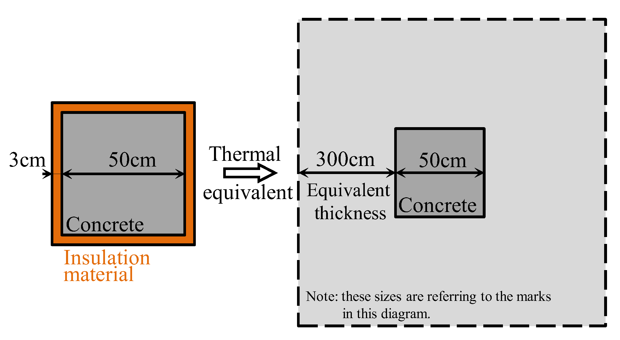
2.1. Specimen Design

To experimentally investigate the temperature field of thin-walled concrete in a green way, the costs and site requirements should be minimized as much as possible. Therefore, by using thermal insulation material, an equivalent experiment was proposed to simulate the thermal state of thin-walled concrete.

In this experiment, a concrete block was designed for temperature measurements, and its lateral surface had a layer of thermal insulation material. The size of the concrete specimen was 50 cm × 50 cm × 40 cm (length × width × thickness); a thickness of 40 cm is the considered maximum influential depth of gradient temperatures in the Chinese specifications JTG D60-2015 [25]. The thermal insulation layer was made of polystyrene with a thickness of 3 cm and a thermal conductivity of 0.03 W/°C/m. If the thermal conductivity of concrete is taken as 3 W/°C/m [26,27], the thermal insulation material can be a thermal equivalent to concrete material with a thickness of 3 m. Therefore, the concrete specimen in this experiment was equivalent to the core part of a thin-walled concrete slab, with just 2% consumption of concrete, as shown in Figure 1. The material components and corresponding proportions of the concrete specimen are detailed in

Table 1. Material components and corresponding proportions in the concrete specimen.

Water–Cement Ratio	Aggregate–Cement Ratio	Sand Ratio	Material Usage/(kg·m−3)
			Water	Cement	Fine Aggregate	Coarse Aggregate	Fly Ash
0.31	3.78	39%	166	477	703.25	1101.75	52

.

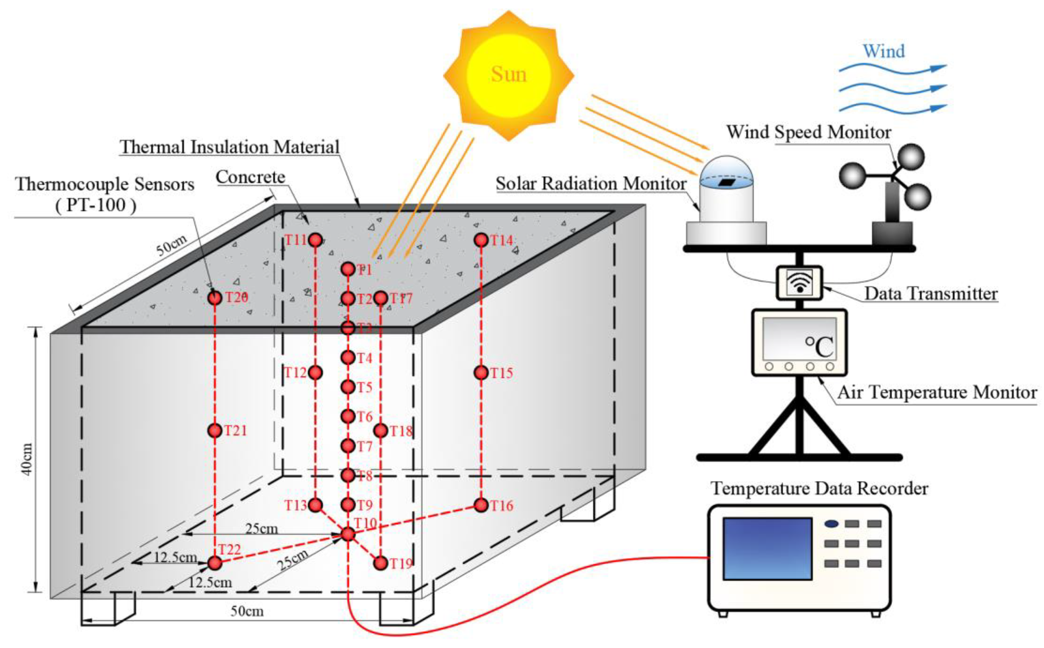
2.2. Experimental Process

The whole experimental process was conducted as shown in Figure 2. The concrete specimen with a lateral insulation layer was placed in a natural environment, while its bottom and top surface were both exposed to the air temperature. Furthermore, the top surface was irradiated with extra solar radiation.

To measure the global temperature field of the concrete specimen, 22 temperature sensors were arranged inside the concrete specimen. The vertical temperature field was measured by T1~T10, which were evenly distributed along the concrete vertical centerline. The horizontal temperature field was measured by surrounding sensors (T11~T22) at the bottom, middle, and top elevations. The PT100 temperature sensors have an accuracy of 0.1 °C.

Meanwhile, the surrounding environmental factors, such as solar radiation, wind speed, and air temperature, were all simultaneously measured and recorded by corresponding monitors. The measurement accuracies for solar radiation, wind speed, and air temperature were 1 W/m, 0.1 m/s, and 0.1 °C, respectively. Moreover, all sensors in the experiment were placed within a distance of 5 m to ensure reliable measurements and all data were recorded at a frequency of every 5 min.

In addition, an open field at Sichuan University (30.55° N, 104.00° E) was chosen to be the experiment site, which was not sheltered by high buildings or trees. The measurement experiment was conducted from April 2022 to April 2023.

3. Measured Temperature Field of Thin-Walled Concrete

3.1. Comparison of Horizontal and Vertical Temperature Fields

To understand the distribution patterns of the temperature field of thin-walled concrete in different directions, the horizontal and vertical temperature fields of the concrete specimen were compared based on the measured data in the hottest month (August 2022) during the experiment process, as shown in Figure 3. During August 2022, the temperatures within each horizontal elevation all presented small differences: the average horizontal temperature differences at the bottom, middle, and top elevations were 0.31 °C, 0.08 °C, and 0.40 °C, respectively. The overall horizontal difference was 0.26 °C. Meanwhile, the reason for the higher temperature of T10 is that it is farther away from the vertical centerline, so it is easier to dissipate heat through lateral convection.

As a comparison, the temperatures at the vertical centerline apparently had various change rules. In terms of the vertical distribution pattern of thin-walled concrete, the temperature at any elevation fluctuated in the form of a sine function, with the temperature of the top surface having the most drastic fluctuations (15 °C in the most extreme situation), while the temperature of the bottom surface was the mildest (4 °C in the most extreme situation). Meanwhile, the average vertical difference between the top and bottom surface was 2.93 °C, which is 11.3 times the horizontal temperature difference.

The most prominent variation in the temperature field of the thin-walled concrete specimen was found in the vertical temperature, and the temperature field of the thin-walled concrete specimen could be assumed to vary in one dimension along the thickness direction. This is consistent with other studies on thin-walled concrete structures. Therefore, this lateral thermal insulation material was verified to be effective in conducting equivalent experiments on thin-walled concrete temperature, and the following temperature analysis was mainly focused on its vertical temperature.

In various design specifications of different countries for bridges or road pavements, such as Chinese JTG D60-2015 [25] and American AATHSO LRDF [28], the vertical temperature is often considered as the main thermal load. According to these specifications, the thin-walled concrete temperature is composed of the mean temperature (T_m) and gradient temperature (T_g), as shown in Figure 4. The mean temperature is the reason for uniform shrinkage or expansion of concrete structures, while the gradient temperature causes uneven bending or twisting. For the experiment in this study, T_m and T_g were calculated using Equation (1).

$$\left\{\begin{array}{l}{T}_{\mathrm{m}}={\displaystyle \sum _{i=1}^{10}(Ti/10)}\\ T_{\mathrm{g}}=T_{\mathrm{measured}}-T_{\mathrm{m}}\end{array}\right.$$

(1)

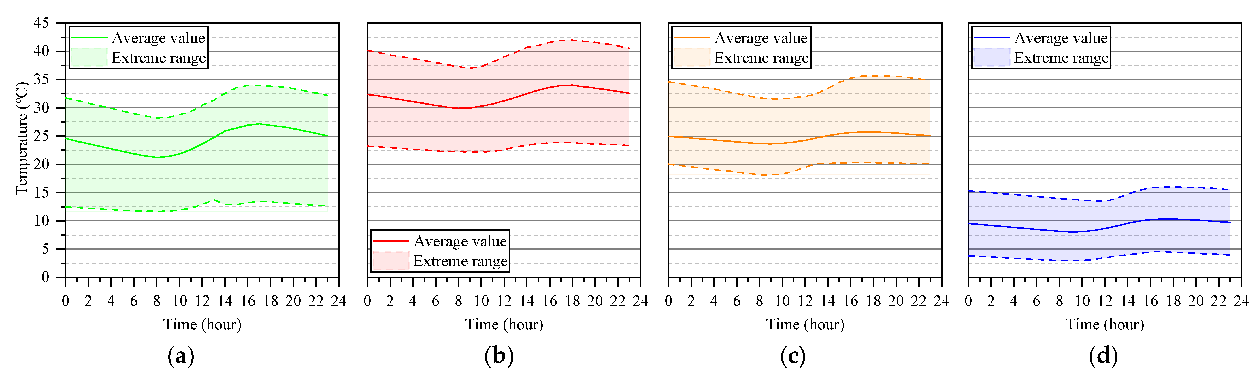
3.2. Seasonal Changes in Mean Vertical Temperature

According to our statistics, the average variation and extreme range within 24 h of the T_m by season are shown in Figure 5. From the perspective of the average value, the T_m in summer was the highest and lowest in winter, and the T_m values in spring and autumn were similar in magnitude. In terms of the width of the range, the T_m in spring had the widest fluctuation range, which was caused by the combined action of cold land and increasing solar radiation. In addition, there was a general rule that fluctuations in T_m within a day showed a sine wave pattern, with the valley usually occurring at 8:00 and the peak occurring at 16:00. The valley values of the T_m in spring, summer, autumn, and winter were, respectively, 11.5 °C, 22.1 °C, 18.2 °C, and 2.8 °C, while the corresponding peak values were 33.8 °C, 42.2 °C, 36.3 °C, and 16.7 °C, respectively.

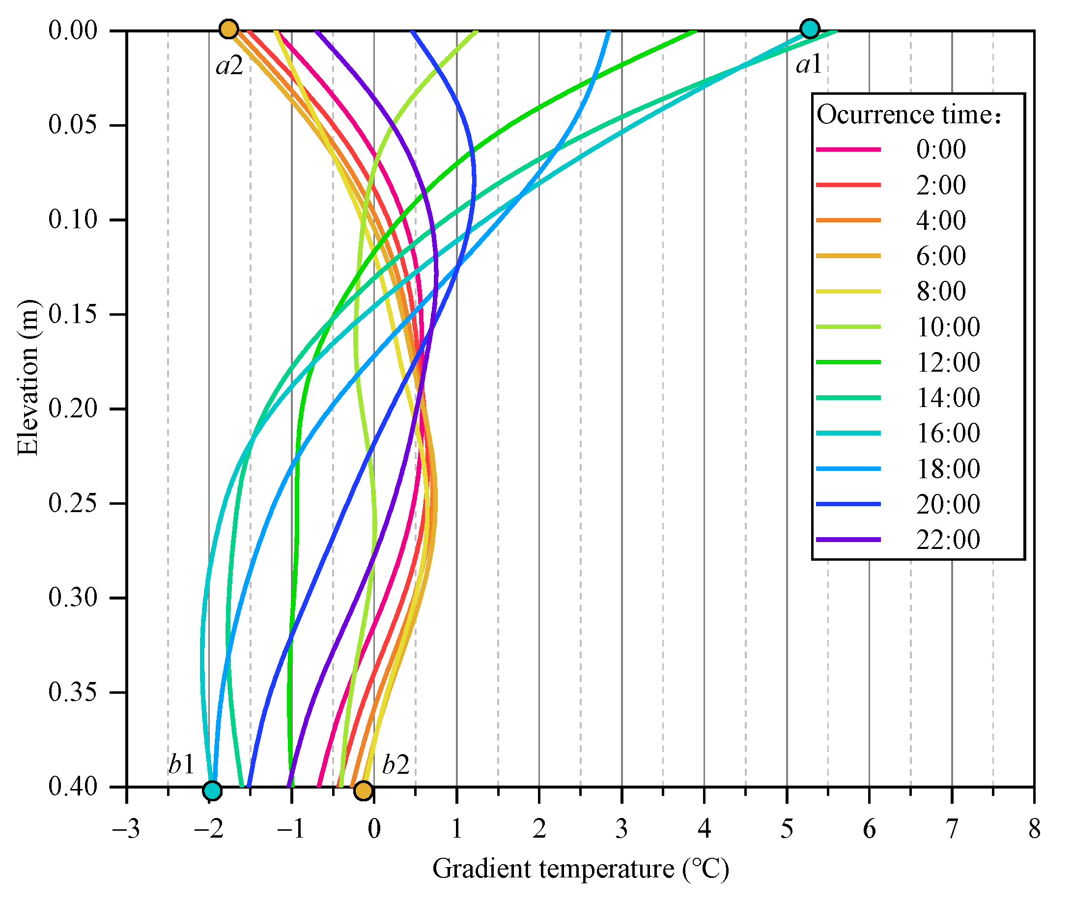
3.3. Seasonal Changes in Vertical Gradient Temperature

The vertical gradient temperature was flexible across both time and space. As shown in Figure 6, the gradient temperature was unevenly distributed along the thickness, and this distribution pattern also changed over time. However, in the field of civil engineering, extreme patterns are more important than the overall changes in gradient temperature. Generally, extreme patterns in the temperature gradient include two patterns with opposite effects. The first one is the maximum positive pattern ($T_{\mathrm{g}}^{+}$), which usually occurs during the day, and the second one is the maximum negative pattern ($T_{\mathrm{g}}^{-}$), which usually occurs at night. Both of them could be identified by the following interpretations.

(1)

$T_{\mathrm{g}}^{+}$ is the gradient temperature pattern when the temperature difference between the top and bottom elevations is the maximum positive value within a day. For example, the gradient temperature pattern at 16:00 in Figure 6 corresponds to the largest value of 7.26 °C within a day (the difference between point a1 and point b1).

(2)

$T_{\mathrm{g}}^{-}$ is the gradient temperature pattern when the temperature difference between the top and bottom elevations is the maximum negative value within a day. For example, the gradient temperature pattern at 6:00 in Figure 6 corresponds to the smallest value of −1.63 °C within a day (the difference between point a2 and point b2).

According to the statistics of the $T_{\mathrm{g}}^{+}$ and $T_{\mathrm{g}}^{-}$ by season, the average variation and extreme range within 24 h by season are shown in Figure 7. Whether from the perspective of the values within or the width of the distribution range, the gradient temperature in summer was the strongest and weakest in winter. Moreover, it was found that, for all seasons, both the $T_{\mathrm{g}}^{+}$ and $T_{\mathrm{g}}^{-}$ could be expressed by an exponential function, as shown in Equation (2), where m is the corresponding gradient temperature value at the bottom elevation (T_gb), while n is the difference between the gradient temperature at the top (T_gt) and T_gb, a is a parameter that needs to be determined, and z is the distance (m) from the top elevation.

$$\left\{\begin{array}{l}{T}_{\mathrm{g}}^{+(-)}=m+n{e}^{-az}\\ m=T_{\mathrm{gb}}\\ n=T_{\mathrm{gt}}-T_{\mathrm{gb}}\end{array}\right.$$

(2)

Multiple data fittings were conducted on the average values of $T_{\mathrm{g}}^{+}$ and $T_{\mathrm{g}}^{-}$, and it was found that a = 11.5 is suitable for both extreme gradient temperature distributions, shown as the dashed lines in Figure 7. Moreover, m and n in different seasons are shown in

Table 2. Value of m and n in different seasons.

Pattern	Parameter	Spring	Summer	Autumn	Winter
$T_{\mathrm{g}}^{+}$	m	−1.64	−1.84	−1.00	−0.37
	n	6.68	7.50	4.62	2.98
$T_{\mathrm{g}}^{-}$	m	0.02	−0.20	0.23	0.45
	n	−1.29	−1.51	−1.83	−2.02

. For $T_{\mathrm{g}}^{+}$, m was always negative but n was the opposite, and there was a correlation between m and n so that m increased when n decreased. For $T_{\mathrm{g}}^{-}$, n was always negative but m did not present a regular change pattern. In general, the most significant $T_{\mathrm{g}}^{+}$ and $T_{\mathrm{g}}^{-}$ values occurred in the summer and winter, respectively. In addition, the $T_{\mathrm{g}}^{-}$ in winter was −0.26 times the $T_{\mathrm{g}}^{+}$ in summer, which is 86.7% and close to the value of −0.3 recommended by AASHTO LRFD [28].

4. Environmental Impact on Temperature Distribution of Thin-Walled Concrete

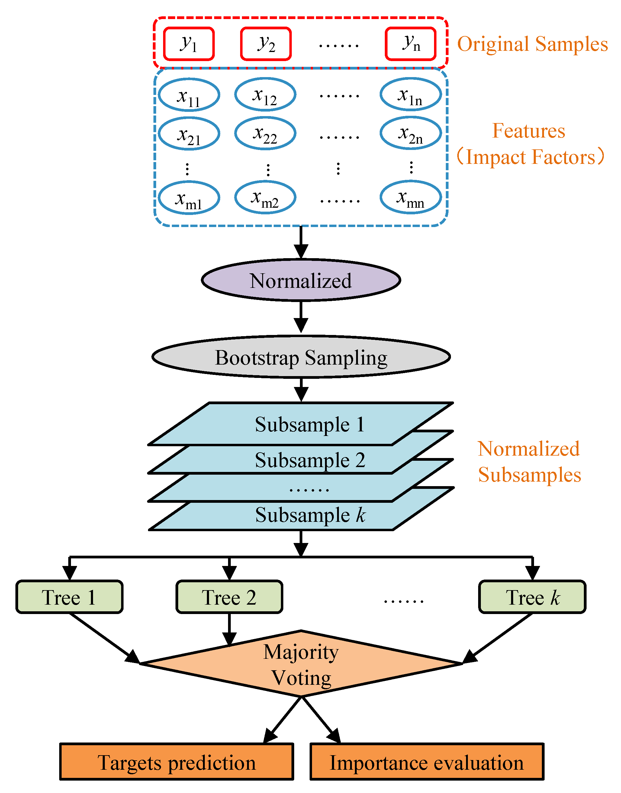
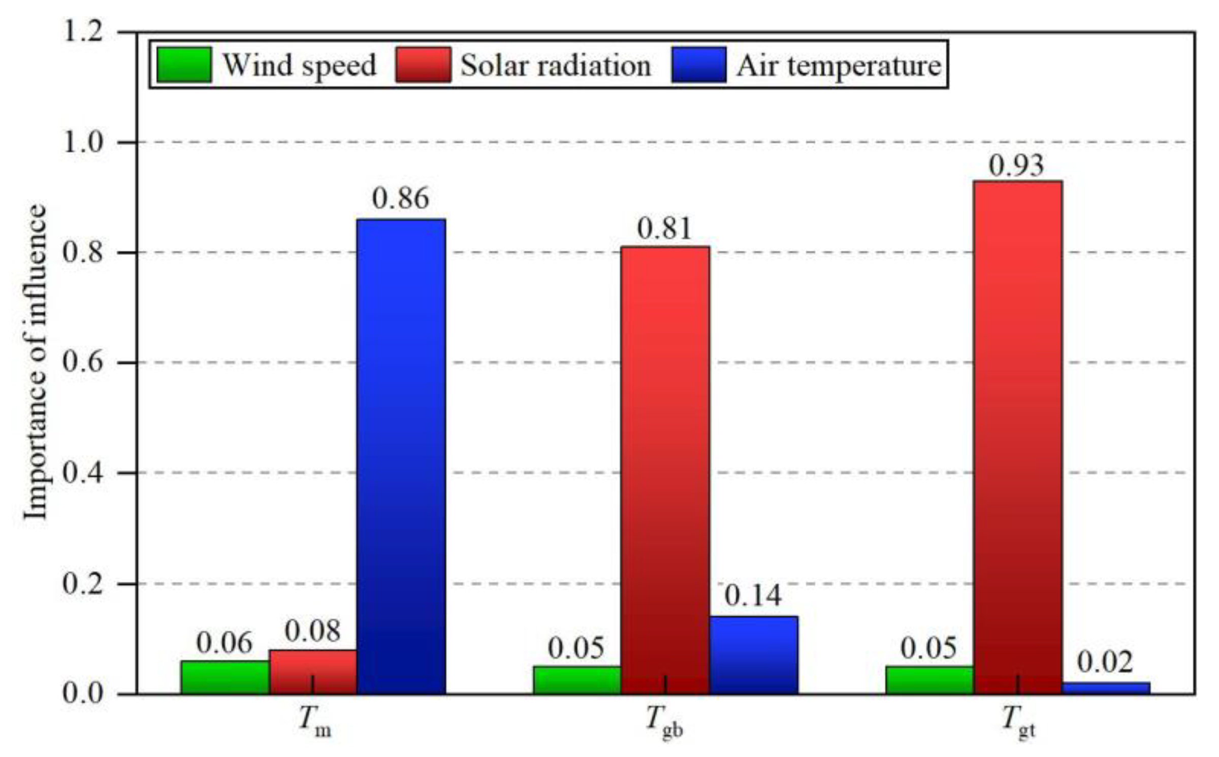
4.1. Sensitivity Analysis of Thin-Walled Concrete to Environmental Factors Based on Random Forest Regression

According to the previous analysis, the temperature distribution composed of the mean temperature and gradient temperature is significantly influenced by environmental factors. Thus, it is necessary to evaluate the impact and importance of each environmental factor. However, due to complex combined effects from various factors, it is difficult to assess and quantify the effects without a powerful tool. Therefore, random forest regression [29,30], as a machine learning method to predict targets and classify multiple parameters in a nonlinear way, was introduced as a powerful statistical tool to conduct the sensitivity analysis of thin-walled concrete to environmental factors.

In this study, random forest regression was performed using MATLAB, and the whole execution process is shown in Figure 8. Firstly, each target in the sample corresponds to several features. The target can be regarded as the dependent variable, and the features as the potential influencing factors. Secondly, all the features were normalized to avoid errors caused by different statistical units. Thirdly, by using bootstrap sampling, the normalized original samples were extracted as multiple random subsamples to establish a forest composed of decision trees. Finally, the prediction of targets and the importance of features were obtained by the majority vote of all the decision trees.

In the practical procedure, the measured environmental factors, including wind speed, solar radiation, and air temperature, were set as features, while T_m, T_gb, and T_gt were set as the three different targets. In addition, to avoid distortion of the results due to transient fluctuations in the measured environmental factors, all data were input as average values throughout the day. By screening the measured data from the experiments, 273 valid samples were obtained. Because the main goal of random forest regression is to search for important factors, all 273 valid samples were used as the training set as well as the test set for RF regression.

To verify the correctness of the algorithm, the measured data were compared to the results of the prediction (Figure 9). For the three targets, all the prediction results were consistent with the measured results. Therefore, both the accuracy and practicality of the random forest regression were verified.

The normalized influence of the environmental factors on T_m, T_gb, and T_gt are illustrated in Figure 10. The influence value of a feature represents its contribution ratio when voting for the prediction, and a larger importance value indicates that the target is more sensitive to the feature. The influence of wind speed was negligible for all the concrete temperature characteristics. Moreover, air temperature and solar radiation produced different effects on the concrete temperature field.

Air temperature was the dominant factor for T_m. Because convection affects both surfaces continuously, it has the ability to heat up the colder surface and cool down the hotter surface. Convection plays a dampening role in the change in concrete temperature, which could make the concrete temperature field approach the air temperature in a relatively uniform way.

Unlike convection, solar radiation only hit the top surface and heated it. Solar radiation acted as a powerful accelerator for the concrete temperature, which could aggravate the uneven distribution of the concrete temperature field. Therefore, T_gb and T_gt were controlled with solar radiation as specific values of the gradient temperature.

4.2. Correlation between Temperature Distribution and Environmental Factors

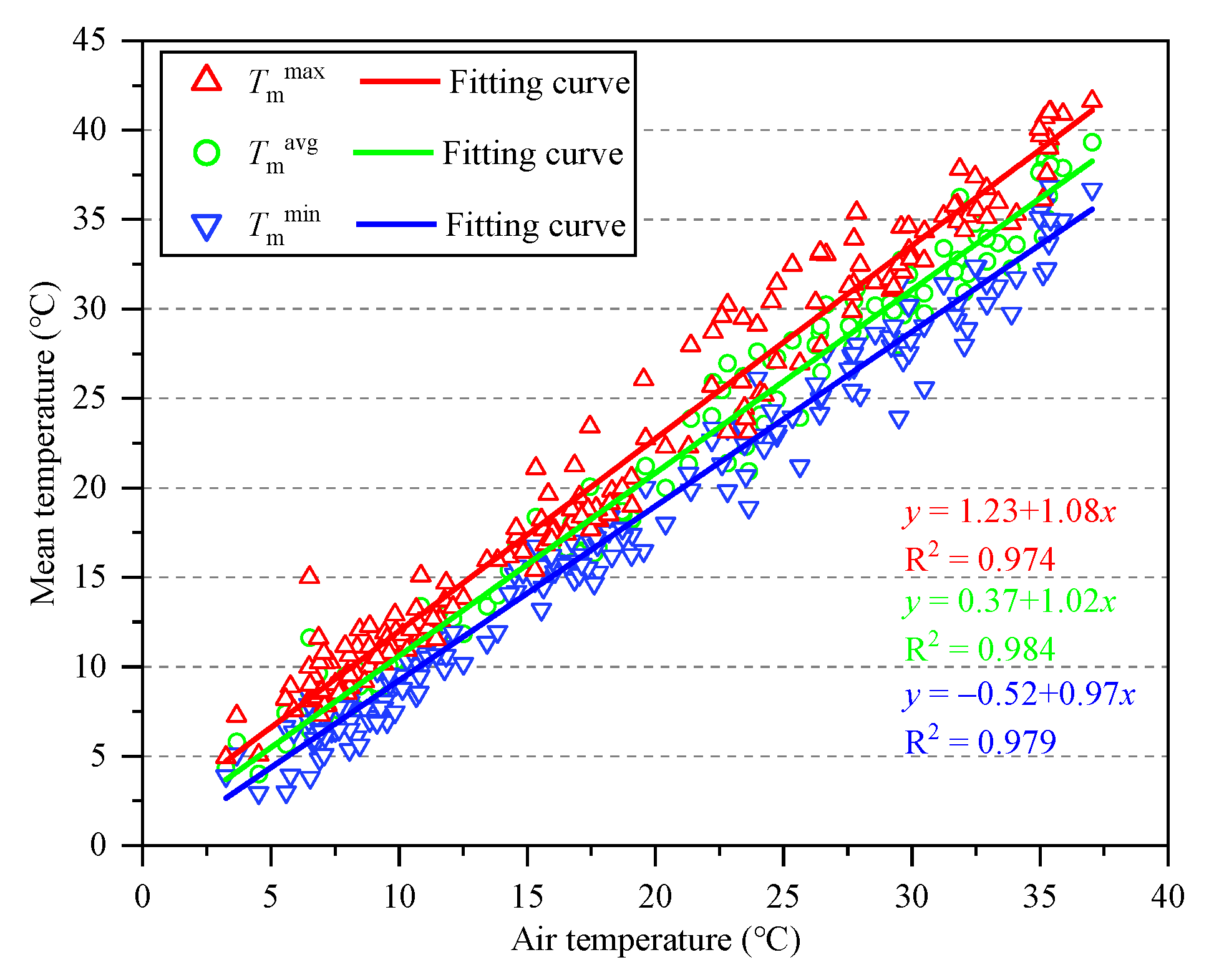
4.2.1. Concrete Mean Temperature and Air Temperature

As per the sensitivity analysis results, air temperature was the main factor that influenced T_m. Thus, the correlation between the mean concrete temperature and the average air temperature should be clarified. The correlations between the average value, as well as the extreme values of T_m, and the average air temperature were drawn, as shown in Figure 11, and the superscripts min, avg, and max represent the minimum, average, and maximum value within a day, respectively. $T_{\mathrm{m}}^{\min }$, $T_{\mathrm{m}}^{\mathrm{avg}}$, and $T_{\mathrm{m}}^{\max }$ were all linearly and positively correlated with the average air temperature. The correlation ratios (°C/°C) were, respectively, 0.97, 1.02, and 1.08, indicating that the higher the average air temperature within a day, the wider the fluctuation range of T_m.

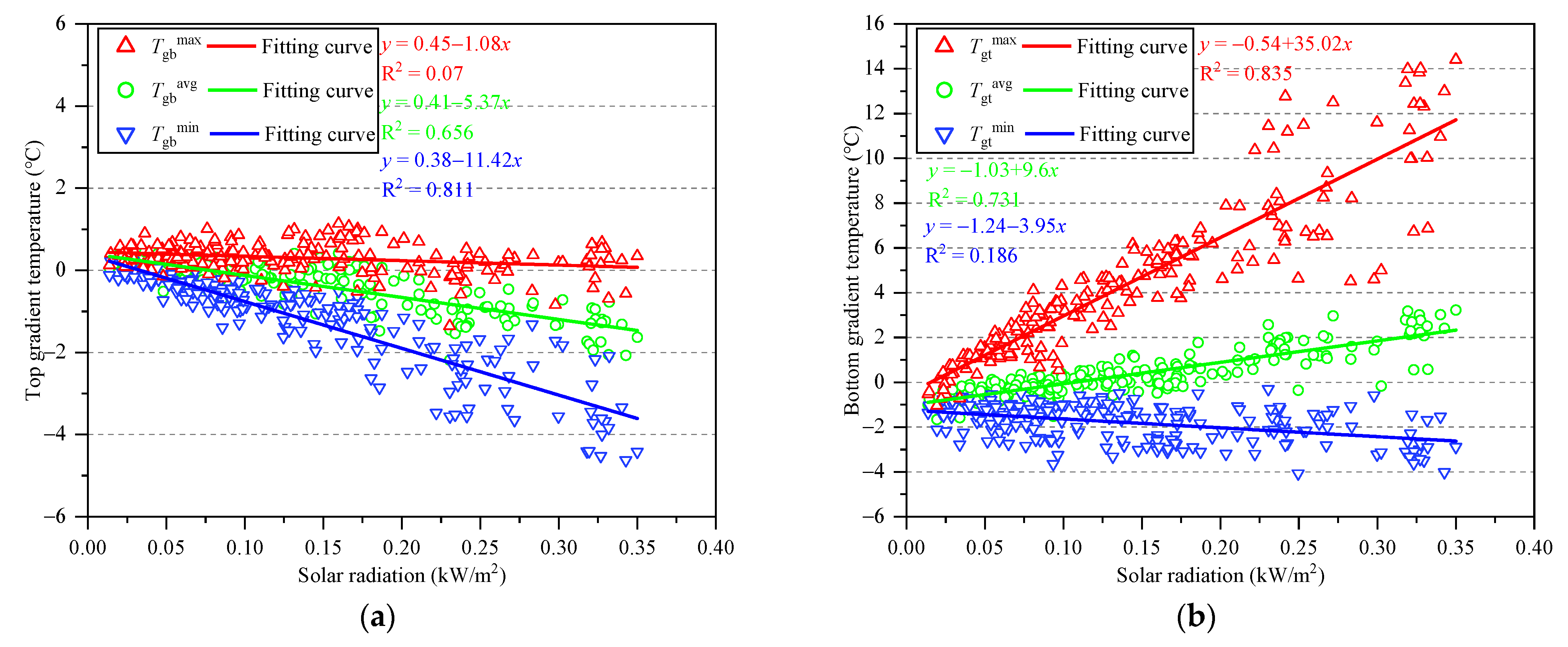
4.2.2. Concrete Gradient Temperature and Solar Radiation

Since both the extreme gradient temperature patterns $T_{\mathrm{g}}^{+}$ and $T_{\mathrm{g}}^{-}$ could be described via T_gb and T_gt, the T_gb and T_gt values were both chosen as the typical cases to be analyzed (Figure 12).

For the bottom surface, $T_{\mathrm{gb}}^{\min }$ and $T_{\mathrm{gb}}^{\mathrm{avg}}$ were both negatively and linearly correlated with the average solar radiation, and the correlation ratios (°C/kW) were −11.4 and −5.37, respectively. Negative correlation ratios showed that strong sunshine increased the temperature of the upper part of the concrete more effectively, so the temperature of the lower part of the concrete increased more slowly compared to the mean temperature. Moreover, there was no correlation between $T_{\mathrm{gb}}^{\max }$ and average solar radiation, so an average $T_{\mathrm{gb}}^{\max }$ value of 0.3 °C was more representative.

Meanwhile, opposite to the bottom surface, $T_{\mathrm{gt}}^{\max }$ and $T_{\mathrm{gt}}^{\mathrm{avg}}$ both had a positive linear correlation with the average solar radiation, and the correlation ratios (°C/kW) were 35.0 and 9.6. Apparently, compared to the bottom surface, the gradient temperature of the top surface was more significantly impacted by solar radiation due to direct irradiation. In addition, $T_{\mathrm{gt}}^{\min }$ was not correlated with the average solar radiation. Therefore, an average $T_{\mathrm{gt}}^{\min }$ value of −1.8 °C was recommended for different solar radiation conditions.

5. Conclusions

A long-term measurement experiment was conducted for thin-walled concrete temperature as well as environmental factors, and the measured data were analyzed using various methods; the detailed conclusions were as follows:

(1)

For green and environmentally friendly resource consumption in the temperature measurement experiment, a concrete block specimen with a layer of thermal insulation material on the lateral surface was used to simulate thin-walled concrete. Furthermore, this method was verified by a result showing that the vertical temperature difference was the dominant difference in the whole temperature field.

(2)

Seasonally, the Tm was highest in summer and lowest in winter, while the T_m in spring had the most drastic fluctuations. Two extreme gradient temperature patterns, $T_{\mathrm{g}}^{+}$ and $T_{\mathrm{g}}^{-}$, occurred in summer and winter, respectively. The $T_{\mathrm{g}}^{-}$ in winter was −0.26 times the $T_{\mathrm{g}}^{+}$ in summer, which is close to the AASHTO LRDF-recommended value. In addition, the $T_{\mathrm{g}}^{+}$ and $T_{\mathrm{g}}^{-}$ in all seasons could be expressed by an exponential function with parameters composed of the corresponding T_gb and T_gt, as well as a = 11.5.

(3)

Random forest regression was applied to analyze the specimen’s sensitivity to environmental factors, which found that wind speed was negligible for the thin-walled concrete temperature field. Moreover, air temperature controlled the concrete Tm, while solar radiation was the dominant factor for T_gb and T_gt.

(4)

Regarding the mean temperature, $T_{\mathrm{m}}^{\min }$, $T_{\mathrm{m}}^{\mathrm{avg}}$, and $T_{\mathrm{m}}^{\max }$ were all linearly and positively correlated with the average air temperature and the correlation ratios (°C/°C) were, respectively, 0.97, 1.02, and 1.08, with a difference of less than 11.3%, indicating that fluctuations in the mean temperature within a day were small.

(5)

The patterns of gradient temperature changes were different for different elevations. For the bottom shadowed surface, $T_{\mathrm{gb}}^{\min }$ and $T_{\mathrm{gb}}^{\mathrm{avg}}$ were both linearly and negatively correlated with the average solar radiation with correlation ratios (°C/kW) of −11.4 and −5.37, respectively. At the top radiated surface, both $T_{\mathrm{gt}}^{\max }$ and $T_{\mathrm{gt}}^{\mathrm{avg}}$ had a positive linear correlation with the average solar radiation, and the correlation ratios (°C/kW) were 35.0 and 9.6, respectively.

References

1. Yang, Y.; Mo, X.; Shi, K.; Wang, Z.-L.; Xu, H.; Wu, Y. Scanning torsional-flexural frequencies of thin-walled box girders with rough surface from vehicles’ residual contact response: Theoretical study. Thin-Walled Struct. 2021, 169, 108332. [Google Scholar] [CrossRef]
2. Reichenbach, S.; Kollegger, J. Detailed Study of Bridges out of Thin Walled Precast Concrete Elements. Procedia Eng. 2016, 156, 388–394. [Google Scholar] [CrossRef]
3. Lu, Z.; Feng, Z.-G.; Yao, D.; Li, X.; Jiao, X.; Zheng, K. Bonding performance between ultra-high performance concrete and asphalt pavement layer. Constr. Build. Mater. 2021, 312, 125375. [Google Scholar] [CrossRef]
4. Baleshan, B.; Mahendran, M. Fire design rules to predict the moment capacities of thin-walled floor joists subject to non-uniform temperature distributions. Thin-Walled Struct. 2016, 105, 29–43. [Google Scholar] [CrossRef]
5. Dang, X.B.; Wan, M.; Zhang, W.-H.; Yang, Y. Stability analysis of the milling process of the thin floor structures. Mech. Syst. Signal Process. 2021, 165, 108311. [Google Scholar] [CrossRef]
6. Chu, Y.; Hou, H.; Yao, Y. Experimental study on shear performance of composite cold-formed ultra-thin-walled steel shear wall. J. Constr. Steel Res. 2020, 172, 106168. [Google Scholar] [CrossRef]
7. Zingoni, A.; Mudenda, K.; French, V.; Mokhothu, B. Buckling strength of thin-shell concrete arch dams. Thin-Walled Struct. 2013, 64, 94–102. [Google Scholar] [CrossRef]
8. Wei, P.; Lin, P.; Peng, H.; Yang, Z.; Qiao, Y. Analysis of cracking mechanism of concrete galleries in a super high arch dam. Eng. Struct. 2021, 248, 113227. [Google Scholar] [CrossRef]
9. Xiao, J.L.; Yang, Y.; Zhuang, L.D.; Nie, X. A numerical and theoretical analysis of the structural performance for a new type of steel-concrete composite aqueduct. Eng. Struct. 2021, 245, 112839. [Google Scholar] [CrossRef]
10. Liu, Y.; Dang, K.; Dong, J. Finite element analysis of the seismicity of a large aqueduct. Soil Dyn. Earthq. Eng. 2017, 94, 102–108. [Google Scholar] [CrossRef]
11. Zhou, W.; Zhang, Z.; Qin, P.; Tian, B.; Zhang, X. Cause analysis of cracks in dual arch dam of Huojia. Jiangxi Hydraul. Sci. Technol. 2023, 49, 50–56. [Google Scholar] [CrossRef]
12. Gu, P.; Wang, L.; Deng, C.; Tang, L. Review of typical failure characteristics of aqueduct structures in China. Adv. Sci. Technol. Water Resour. 2017, 37, 1–8. [Google Scholar] [CrossRef]
13. Li, Y.; Nie, L.; Wang, B. A numerical simulation of the temperature cracking propagation process when pouring mass concrete. Autom. Constr. 2014, 37, 203–210. [Google Scholar] [CrossRef]
14. Chen, B. Research on the Internal Thermal Boundary Conditions of Concrete Closed Girder Cross-Sections under Historically Extreme Temperature Conditions. Appl. Sci. 2020, 10, 1274. [Google Scholar] [CrossRef]
15. Zhou, Y.; Bai, L.; Yang, S.; Chen, G. Simulation Analysis of Mass Concrete Temperature Field. Procedia Earth Planet. Sci. 2012, 5, 5–12. [Google Scholar] [CrossRef]
16. Zhang, C.; Liu, Y.; Liu, J.; Yuan, Z.; Zhang, G.; Ma, Z. Validation of long-term temperature simulations in a steel-concrete composite girder. Structures 2020, 27, 1962–1976. [Google Scholar] [CrossRef]
17. Lu, Y.; Li, D.; Wang, K.; Jia, S. Study on Solar Radiation and the Extreme Thermal Effect on Concrete Box Girder Bridges. Appl. Sci. 2021, 11, 6332. [Google Scholar] [CrossRef]
18. Fan, J.S.; Liu, Y.F.; Liu, C. Experiment study and refined modeling of temperature field of steel-concrete composite beam bridges. Eng. Struct. 2021, 240, 112350. [Google Scholar] [CrossRef]
19. Liu, C.; Xiao, J.; Ma, K.; Xu, H.; Shen, R.; Zhang, H. Experimental and numerical investigation on the temperature field and effects of a large-span gymnasium under solar radiation. Appl. Therm. Eng. 2023, 225, 120169. [Google Scholar] [CrossRef]
20. Wang, Y.; Zhu, J.; Guo, Y.; Wang, C. Early shrinkage experiment of concrete and the development law of its temperature and humidity field in natural environment. J. Build. Eng. 2023, 63, 105528. [Google Scholar] [CrossRef]
21. Larsson, O.; Thelandersson, S. Estimating extreme values of thermal gradients in concrete structures. Mater. Struct. 2011, 44, 1491–1500. [Google Scholar] [CrossRef]
22. Liu, P.; Yu, Z.; Guo, F.; Chen, Y.; Sun, P. Temperature response in concrete under natural environment. Constr. Build. Mater. 2015, 98, 713–721. [Google Scholar] [CrossRef]
23. Liu, J.; Liu, Y.; Jiang, L.; Zhang, N. Long-term field test of temperature gradients on the composite girder of a long-span cable-stayed bridge. Adv. Struct. Eng. 2019, 22, 2785–2798. [Google Scholar] [CrossRef]
24. Liu, J.; Liu, Y.; Zhang, G. Experimental Analysis of Temperature Gradient Patterns of Concrete-Filled Steel Tubular Members. J. Bridge Eng. 2019, 24, 04019109. [Google Scholar] [CrossRef]
25. JTG D60-2015; General Specifications for Design of Highway Bridges and Culverts. China Communications Press: Beijing, China, 2015.
26. Shafigh, P.; Asadi, I.; Mahyuddin, N.B. Concrete as a thermal mass material for building applications—A review. J. Build. Eng. 2018, 19, 14–25. [Google Scholar] [CrossRef]
27. Asadi, I.; Shafigh, P.; Hassan, Z.F.A.B.; Mahyuddin, N.B. Thermal conductivity of concrete—A review. J. Build. Eng. 2018, 20, 81–93. [Google Scholar] [CrossRef]
28. AASHTO. LRFD Bridge Design Specifications, 8th ed.; AASHTO: Washington, DC, USA, 2017. [Google Scholar]
29. Antoniadis, A.; Lambert-Lacroix, S.; Poggi, J.M. Random forests for global sensitivity analysis: A selective review. Reliab. Eng. Syst. Saf. 2021, 206, 107312. [Google Scholar] [CrossRef]
30. Auret, L.; Aldrich, C. Empirical comparison of tree ensemble variable importance measures. Chemom. Intell. Lab. Syst. 2011, 105, 157–170. [Google Scholar] [CrossRef]
Figure 1. Diagram of the thermal equivalent process.
Applsci 13 12157 g001
Figure 2. Diagram of the measurement tests for concrete temperature and environmental factors.
Applsci 13 12157 g002
Figure 3. Comparison of horizontal and vertical temperature differences. (a) Horizontal temperature; (b) vertical temperature.
Applsci 13 12157 g003
Figure 4. Diagram of temperature distribution components.
Applsci 13 12157 g004
Figure 5. Seasonal vertical mean temperature Tm: (a) in spring, from March to May; (b) in summer, from June to August; (c) in autumn, from September to November; and (d) in winter, from December to February.
Applsci 13 12157 g005
Figure 6. Flexible gradient temperature (average values during summer 2022).
Applsci 13 12157 g006
Figure 7. Seasonal changes in extreme vertical gradient temperature  T g +  and  T g : (a) in spring; (b) in summer; (c) in autumn; and (d) in winter.
Applsci 13 12157 g007
Figure 8. Execution diagram of random forest regression.
Applsci 13 12157 g008
Figure 9. Comparison of the measured data with the results predicted by random forest regression: (a) Tm; (b) Tgb; (c) Tgt.
Applsci 13 12157 g009
Figure 10. Influence of environmental factors on Tm, Tgb and Tgt.
Applsci 13 12157 g010
Figure 11. Correlation between the concrete mean temperature and air temperature.
Applsci 13 12157 g011
Figure 12. Correlation between the concrete gradient temperature and solar radiation: (a) bottom elevation; (b) top elevation.
Applsci 13 12157 g012