Static Wind Reliability Analysis of Long-Span Highway Cable-Stayed Bridge in Service

Abstract

Long-span cable-stayed bridge is a typical wind-sensitive structure because of its light weight and great flexibility. The reliability evaluation of the cable-stayed bridge under wind action becomes a key issue during bridge design and operation. In this paper, taking Xiangshan Harbor highway cable-stayed bridge in Ningbo City in China as the engineering background, ANSYS 15.0 is used to build a finite element model of this bridge to explore its aerostatic stability and influencing parameters, then the static wind reliability of this bridge is analyzed. Firstly, considering the structural nonlinearity and the nonlinearity of static wind load comprehensively, the critical wind speed of aerostatic instability of the Xiangshan Harbor cable-stayed bridge is calculated by the internal and external double iteration method. Then the influence of the initial wind attack angle, steel wire breakage rate of the stay cables, static three-component force coefficients, and cable broken position on the static wind stability of this bridge are discussed. Thus, the variation rule of the critical aerostatic instability wind speed is obtained, and the parameter that has the greatest impact on the static wind stability of the cable-stayed bridge in service is determined. Finally, considering the randomness of these key parameters, they are treated as random variables, Latin hypercube sampling (LHS) method is used to obtain samples of random variables to calculate aerostatic instability wind speed for a given sample by self-written calculation program, and on this basis, static wind reliability analysis is conducted by the checking point method, which provides strong support for the static wind risk evaluation of the existing long-span cable-stayed bridge.

1. Introduction

With the increasing main span lengths in modern cable-stayed bridges, it is very necessary to conduct a comprehensive analysis and evaluation of their wind-resistant performance. Generally speaking, flutter has been widely considered because it is more prone to occur in bridge design, especially for long-span bridges [1,2,3,4]. However, when there are more and more bridges with a main span exceeding 1000 m, aerostatic stability also becomes a primary factor which can be even more leading than the flutter instability in some projects, especially for cable-stayed bridges [5]. Static wind instability of bridges is caused by the interaction with the deformation of bridges and static wind loads [5,6]. Hirai observed the torsional divergence caused by the static wind in the wind tunnel test of the suspension bridge in 1967 [7]. The researchers from Tongji University have also observed the static wind instability phenomenon of Shantou Bay No. 2 cable-stayed bridge through wind tunnel test and Jiang Yin suspension bridge [8,9]. Boonyapinyo [10,11] explored and improved the static wind instability of bridges, and preliminarily discovered the static wind instability mechanism. Other scholars [12,13,14] also analyzed and discussed the aerostatic stability of long-span bridges, taking into account the nonlinearity of the bridge structure and the uncertainty of parameters.

The in-depth research on the static wind instability of long-span bridges by the above-mentioned scholars has helped people to understand the mechanism of static wind instability more profoundly, and also promoted subsequent scholars to conduct further research on basis of reliability theory for the static wind instability of long-span bridges. At present, there are many studies on the static wind reliability of long-span bridges using the deterministic analysis method. Su [15] used the Mont Carlo method to explore the reliability of the static wind stability of bridges. Li [16] explored the influence of different parameters on the static wind stability of long-span suspension bridges. Frangopol [17,18] evaluated the reliability of long-span suspension bridges in Japan, considering the influence of the geometric nonlinearity of structures. Chen [19] took the long-span cable-stayed bridge as the background, and focused on the reliability theory and its calculation method to make the system more complete. Liang [20] conducted a static wind reliability analysis on a steel truss suspension bridge, and considered the influence of factors such as the initial wind attack angle and the wind-resistant cable structure with or without a central buckle. These scholars all use the deterministic analysis method to analyze the static wind stability of bridges. But in practice, the uncertainty of some parameters such as structural parameters, wind speed, aerodynamic coefficients, and so on, has a great influence on the aerostatic instability of long-span cable-stayed bridges. In addition, the actual service conditions of existing bridges shall also be considered. As a result, the deterministic method for static wind instability analysis is not comprehensive, it is very necessary to conduct static wind reliability analysis on long-span cable-stayed bridges based on parameter uncertainty.

Based on the previous research, the actual conditions of cable-stayed bridges in service, and the factors that may affect the static wind stability, in this paper the randomness of the three key parameters i.e., the static three-component force coefficient, the steel wire breakage rate of the stay cables and the broken position of stay cables is considered and Latin hypercube sampling method is used to randomly obtain the samples of these parameters according to their distribution. Then the critical aerostatic instability wind speed of the Xiangshan Harbor Bridge in service is calculated, and the checkpoint method is adopted to analyze the static wind reliability to obtain reliability indexes and failure probability considering the probability distribution of actual wind speed, which provides strong support for the static wind risk analysis and evaluation of the existing long span cable-stayed bridge.

2. Reliability Theory of Static Wind Instability Analysis for Bridges

2.1. Aerostatic Instability Analysis Theory for Bridges

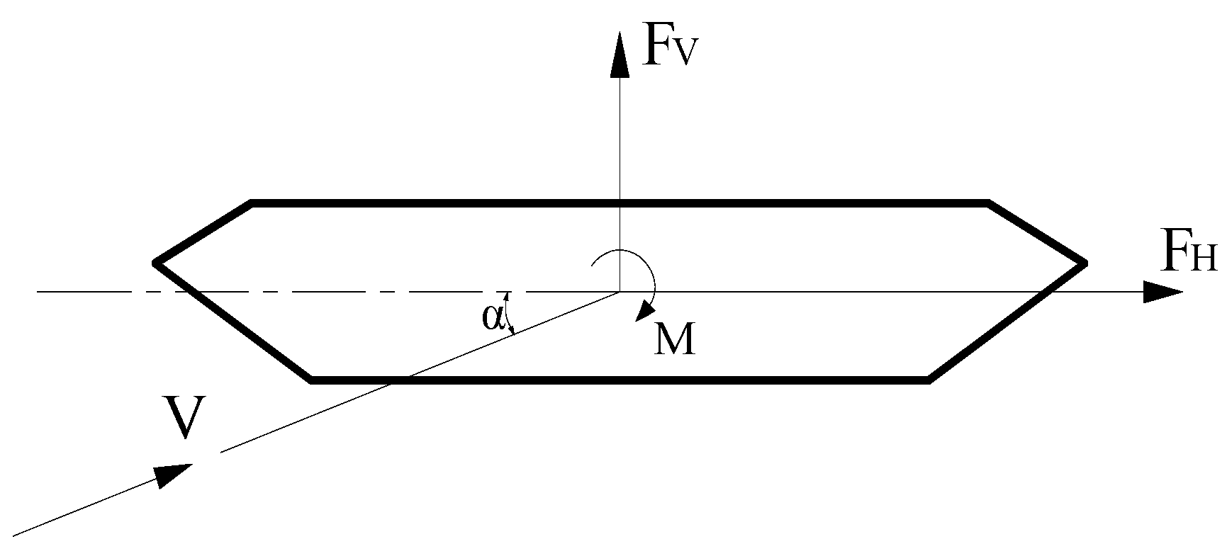
2.1.1. Static Wind Load Calculation on Bridges

(1)

Static wind load on main girders

At present, the established nonlinear theory of static wind load refers to that the main girder section will be twisted under static wind load which causes the effective wind attack angle to change, and the change of the effective wind attack angle will also cause the variation of the static three-component force coefficient. Therefore, the final static wind forces acting on the main beam should be the actual static wind forces after modifying the deformation of the main beam. The static wind force can be described in the body axis coordinate system, namely, the coordinate system is represented along the main beam with the cross-section centroid as the origin and the directions of the coordinate axes are parallel or perpendicular to the bridge deck in Figure 1 below, then the static wind forces on the main girder are calculated by Equation (1).

$$\begin{gathered} F_H\left(\alpha \right)=\frac{1}{2}\rho V^2{C}_H\left(\alpha \right)D \\ {F}_V\left(\alpha \right)=\frac{1}{2}\rho V^2{C}_V\left(\alpha \right)B \\ M\left(\alpha \right)=\frac{1}{2}\rho V^2{C}_M\left(\alpha \right)B^2 \end{gathered}$$

(1)

where $C_H\left(\alpha \right)$, $C_V\left(\alpha \right)$ and $C_M\left(\alpha \right)$ are the drag, lift, and torsion moment coefficient of the beam section in the body axis coordinate system when the wind attack angle is α, respectively; $F_H\left(\alpha \right)$, $F_V\left(\alpha \right),$ and $F_M\left(\alpha \right)$ are the drag force, lift force, and torsion moment per unit length at the centroid of the main beam section in the same coordinate system when the wind attack angle is α, respectively; D and B are the lateral projection height and width of the main beam section, respectively; α is the effective wind attack angle, when the incoming wind direction is diagonally upward, the wind attack angle is positive, otherwise the wind attack angle is negative; ρ is the air density (kg/m³), equals to 1.25 kg/m³ in this research, and V is the equivalent static gust wind speed at the bridge site.

The static three-component force coefficient including the drag coefficient, lift coefficient, and torsion moment coefficient of the main beam section in Equation (1) is obtained from the segmental model wind tunnel test. For the cross-section of the main beam in the Xiangshan Harbor highway cable-stayed bridge, the variation curve of the aerodynamic force coefficient with the wind attack angle [21] is shown in Figure 2.

(2)

Static wind load on stay cables

According to the different wind directions, the wind load acting on the stay cables is divided into the transverse wind load perpendicular to the driving direction of the bridge and the longitudinal wind load along the bridge direction. In actual projects, the wind load in the lateral direction is often an important factor for the aerostatic stability of the bridge, so only the wind load in the lateral bridge direction is considered for the stay cables.

According to the “Wind-resistant Design Specification for Highway Bridges” (JTG/T 3360-01-2018) [22] in China, the wind force on the stay cables is calculated by the following formula under the action of the lateral wind:

$$F_H=\frac{1}{2}\rho V^2{C}_H{A}_n$$

(2)

where F_H is the static wind force on the stay cable under the action of the lateral wind; C_H is the drag coefficient of the stay cable which can be taken as 0.8 when calculating the static wind stability of the bridge; A_n is the projected area of the stay cable in downwind direction which can be calculated by multiplying the diameter by the downwind projection height of the stay cable.

(3)

Static wind load on piers and pylons

Under the action of static wind, the piers and pylons have a small deformation due to their high flexural rigidity along the longitudinal direction of the bridge. Therefore, only the effect of the transverse wind on the piers and pylons is considered, and the calculation formula is the same as Equation (2), where A_n is the projected area of the corresponding bridge components in downwind direction, C_H is the drag coefficient of the components. The drag coefficients of the piers and pylons can be determined according to Table 5.4.2-1 in the “Wind-resistant Design Specification for Highway Bridges” (JTG/T 3360-01-2018) [22] in China, but if the section of the piers and pylons are complex, the coefficient should be got by boundary layer wind tunnel test or computational fluid dynamic simulation.

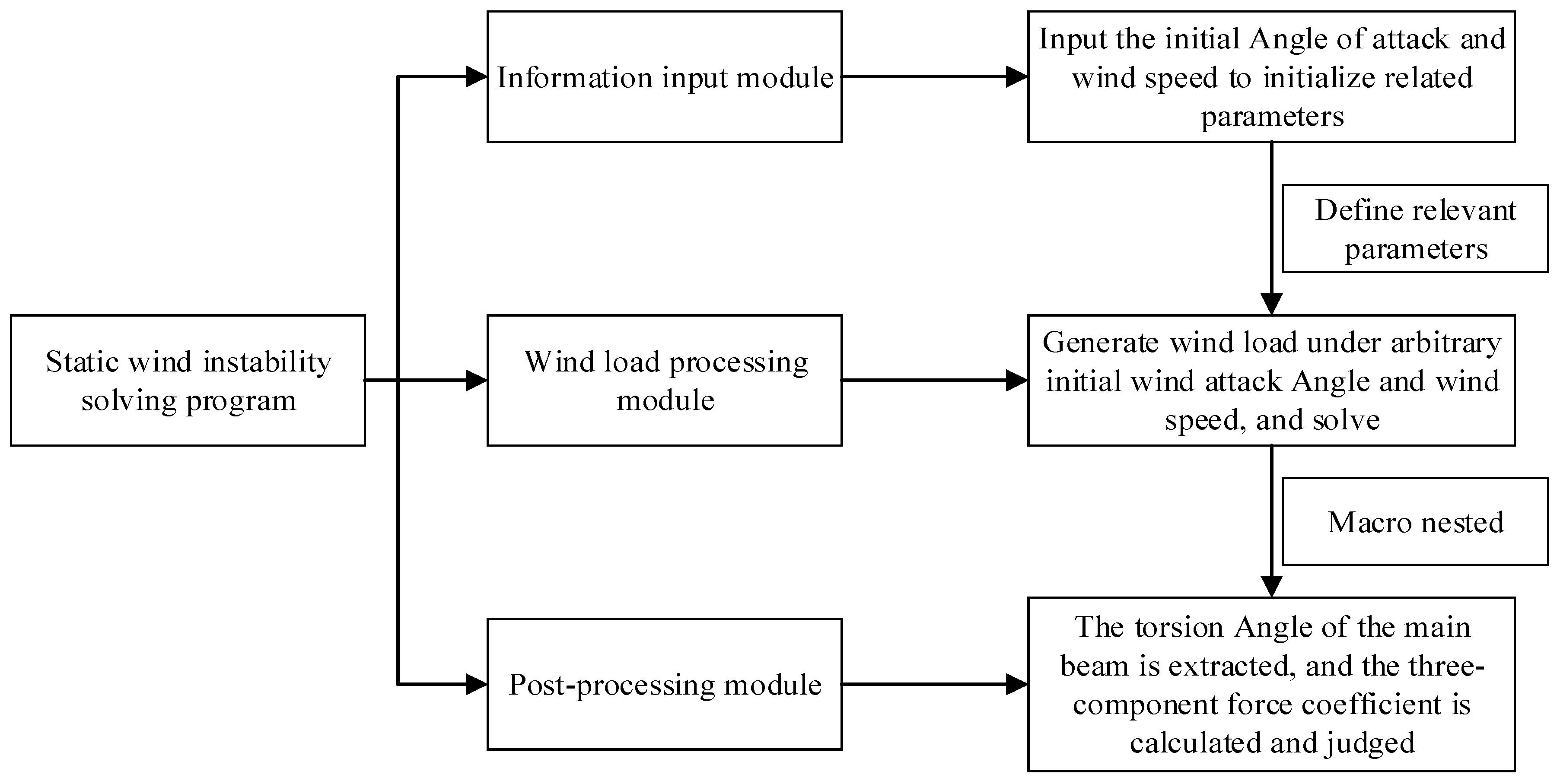
2.1.2. Calculation of Aerostatic Instability wind Speed of Bridges

So far, the accepted solution method for the aerostatic instability wind speed of bridges is the UL incremental method [23], that is, a method combining the incremental method with the internal and external two-iterative procedure is used to solve the nonlinear incremental equation to obtain the displacement response of the bridge. When increasing the static wind speed based on a predetermined step size, the iteration in the inner layer finishes the geometric nonlinear calculation of the bridge structure, and the iteration in the outer layer finds the equilibrium position of the bridge structure under this wind speed. The specific process is as follows [8]:

(1)

Assume the initial static wind speed V₀, and the initial wind attack angle α;

(2)

Calculate the static wind force acting on each bridge component including the main girder, stay cables, piers, and pylons at current wind speed and wind attack angle;

(3)

Establish the finite element model of the bridge, then apply the static wind load calculated in step (2) to each member of the bridge, and the Newton-Rapson method is adopted to solve the static response of the bridge such as the lateral displacement ($U_x$), vertical displacement ($U_y$) and torsion angle (Rot_z) of each node of the main girder at current wind speed and wind attack angle;

(4)

Extract the maximum torsion angle of the main girder from the calculation result in step (3), and recalculate the static wind load on the bridge considering the variation of the wind attack angle;

(5)

Judge whether the Euclidean norm of the three-component force coefficient is no more than the allowable value:

$${\left\{\frac{{\sum }_{j=1}^N{[C_k\left({\alpha }_j\right)-C_k({\alpha }_{j-1})]}^2}{{\sum }_{j=1}^N{[C_k\left({\alpha }_{j-1}\right)]}^2}\right\}}^{1/2}\le {\epsilon }_k\left(k=H,V,M\right)$$

(3)

where $C_k\left({\alpha }_j\right)$ is the three-component force coefficient corresponding to the effective wind attack angle ${\alpha }_j$ of each node of the main girder after applying the jth static wind load; $C_k\left({\alpha }_{j-1}\right)$ is the result after applying the (j − 1)th static wind load; N is the total number of nodes on the main girder in the finite element model of the bridge; ${\epsilon }_k$ is the allowable value of the Euclidean norm of the three-component force coefficient which is taken as 5%.

(6)

If all three-component force coefficients are less than the allowable value ${\epsilon }_k$, improve the wind speed in accordance with the predetermined step size ($\Delta v=20 \mathrm{m}/\mathrm{s}$ in this research), and repeat steps (2)~(5), otherwise repeat steps (3)~(5);

(7)

If the number of iterations is greater than a predetermined time at a certain wind speed, the convergence requirement is still not satisfied, restore the previous wind speed, shorten the step size of the wind speed and recalculate, until the difference between the two adjacent wind speeds is no more than the predetermined value.

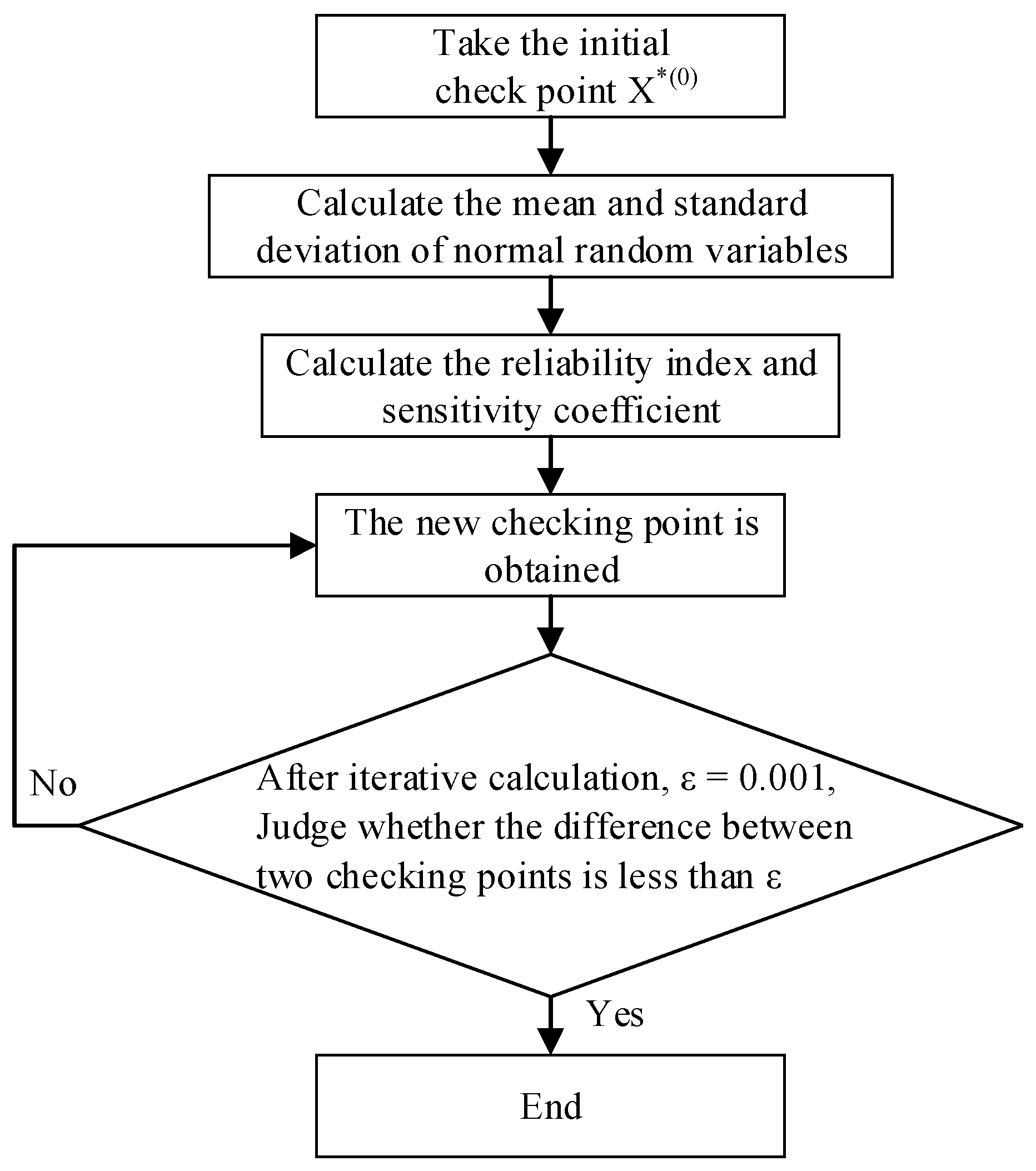
2.2. Theory and Method of Reliability Analysis

The checkpoint method is often used for reliability analysis [24]. When the value of the random variable is at the checkpoint, the structure is in the most unfavorable state. At this moment, the functional function reaches an extreme value, namely, the failure probability of the structure is the largest at this checkpoint. It is worth noting that, before adopting the checkpoint method, if the random variables do not obey the normal distribution, they must be equivalently normalized according to the failure domain area must be equal before and after the equivalent normalization. Note the coordinate value of the checkpoint as $x_i^{*}\left(i=1,2,\cdots ,n\right)$, thus the expressions of the equivalent normalization condition are:

$$F_{X_i}(x_i^{*})=\Phi \left\{\frac{x_i^{*}-{\mu }_{X_i}^{\prime }}{{\sigma }_{X_i}^{\prime }}\right\}$$

(4)

$$f_{X_i}(x_i^{*})=\frac{\phi \left\{\frac{x_i^{*}-{\mu }_{X_i}^{\prime }}{{\sigma }_{X_i}^{\prime }}\right\}}{{\sigma }_{X_i}^{\prime }}$$

(5)

in which, $F_{X_i}$ stands for the distribution function for non-normal random variables; $\Phi$ stands for the standard normal distribution function; $f_{X_i}$ stands for the density function for non-normal random variables;$\phi$ stands for the density function of $\Phi$; ${\mu }_{X_i}^{\prime }$ stands for the average value of the equivalent normal variable $X_i^{\prime }$ and ${\sigma }_{X_i}^{\prime }$ stands for the variance of the equivalent normal random variable $X_i^{\prime }$. Based on Equations (4) and (5), the average value and variance of the equivalent normal random variable $X_i^{\prime }$ can be obtained as:

$$\left\{\begin{array}{l}{\mu }_{X_i}^{\prime }=x_i^{*}-{\Phi }^{-1}\left[F_{X_i}\left(x_i^{*}\right)\right]{\sigma }_{X_i}^{\prime }\\ {\sigma }_{X_i}^{\prime }=\phi \left({\Phi }^{-1}\left[F_{X_i}\left(x_i^{*}\right)\right]\right)/f_{X_i}\left(x_i^{\prime }\right)\end{array} \right.$$

(6)

According to the above transformation method, if the random variable X obeys the log-normal distribution, that is, $Y=\mathit{ln}X$, $Y~N\left(\mu Y,{\sigma }^{2}Y\right)$, the average value and standard deviation of the normal random variable is calculated as follows:

$$\left\{\begin{array}{l}{\mu }_Y={\mu }_{lnX}=\mathit{ln}(\frac{{\mu }_X}{\sqrt{1+{\delta }_X^2}})\\ {\sigma }_Y={\sigma }_{lnX}=\sqrt{\mathit{ln}(1+{\delta }_X^2)}\end{array}\right.$$

(7)

where ${\mu }_X$ is the average value of the random variable X, ${\sigma }_X$ is the standard deviation of random variable X, and ${\delta }_X$ is the variation coefficient of random variable X.

Let $Z=g\left(X_1,\cdots X_n\right)$ as the functional function and $x_i^{*}$ as the design checkpoint, thus the expression of the reliability index $\beta$ can be written as:

$$\beta \approx \frac{g_X\left(x_1^{*},x_2^{*},\cdots ,x_n^{*}\right)+{\left.{\sum }_{i=1}^n\frac{\partial g_X}{\partial X_i}\right|}_{x_i^{*}}\left(u_{X_i}-x_i^{*}\right)}{\sqrt{{\left.{\sum }_{i=1}^n(\frac{\partial g_X}{\partial X_i}\right|}_{x_i^{*}}{\sigma }_{X_i}{)}^2}}$$

(8)

By introducing the sensitivity coefficient $a_i$, let:

$$a_i=\cos {\theta }_i=\frac{{\left.\frac{\partial g_X}{\partial X_i}\right|}_{x_i^{*}}{\sigma }_{X_i}}{\sqrt{{\sum }_{i=1}^n{\left.(\frac{\partial g_X}{\partial X_i}\right|}_{x_i^{*}}{\sigma }_{X_i}{)}^2}}$$

(9)

Then there is the following relationship between $x_i^{*}$ and $\beta$:

$$x_i^{*}={\mu }_{x_i}-{\sigma }_{x_i}\beta a_i$$

(10)

The flow chart of structural reliability calculation by checking point method is shown in Figure 3.

To ensure the randomness of the parameters affecting the static wind response of the bridge, in this research, the Latin Hypercube Sampling (LHS) method is used to extract the sample of these random parameters, which is a highly efficient and fast sampling method and is a further improvement based on stratified sampling method. The advantage of this method is to greatly reduce the number of samplings while meeting the accuracy requirements. Bao [25] pointed out that the number of samples required by the Latin hypercube sampling method is only about 1/4 of that of the traditional sampling method to obtain the failure probability with the same accuracy. This can save a lot of time cost during the numerical simulation calculation of structural reliability. In the subsequent analysis, Latin hypercube sampling is used for the parameter sampling and combines with the checkpoint method for reliability calculation to obtain the static wind reliability indexes of the bridge which can greatly reduce time improve the calculation efficiency, and ensure accuracy.

3. Functional Function and Parameter Distribution for Aerostatic Instability Analysis

3.1. Functional Function of Static Wind Instability

If the whole structure or a part of the structure exceeds a specific condition, the structure won’t meet a specified functional requirement in the design or operation stage. This specific condition is called the limit state of the structure which is at the dividing point of structure reliability and unreliability. The calculation of structural reliability is to judge whether the structure reaches the limit state. For reliability analysis of bridges under static wind load, the limit state function Z is described by the difference between the actual critical aerostatic instability wind speed $U_{cr}$ and the design wind speed $U_m$ of the bridge, it is written as:

$$Z=U_{cr}-U_m$$

(11)

Through Equation (11), it can be found that the bridge structure will suffer from wind-induced static instability damage when the actual critical instability wind speed of the bridge is less than the design wind speed. In Equation (11), the design wind speed $U_m$ can be calculated by the gust coefficient multiplied by the 10 min average wind speed at the bridge site, namely:

$$U_m=G_v{U}_b$$

(12)

where $U_b$ stands for the 10 min average wind speed at the height of the main girder and $G_v$ stands for the gust coefficient reflecting the influence of wind speed fluctuation, they are essentially random variables, which both need to be described by the probability distribution and mathematical statistics methods.

$U_{cr}$ stands for the actual critical aerostatic instability wind speed of the bridge, and it should be corrected by a factor $C_w$ because of the randomness of the natural wind, structural parameters, and calculation model of the bridge structure, namely:

$$U_{cr}=C_w{U}_s$$

(13)

where $U_s$ is the calculated critical aerostatic instability wind speed determined by finite element analysis, and $C_w$ is the correction factor for static wind instability critical wind speed which is also a random variable and should also be represented by the probability distribution and mathematical statistics methods similar to $G_v$.

Finally, the functional function for the aerostatic reliability analysis of the bridge structure is further written as:

$$Z=C_w{U}_s-G_v{U}_b$$

(14)

3.2. Probability Distribution Function of Wind Speed at Bridge Site

According to the statements in Wind-resistant Design Specification for Highway Bridges (JTG/T 3360-01-2018) in China: “When the weather station in the area where the bridge is located has sufficient unmeasured data of continuous wind speed, the probability distribution type of annual maximum wind speed of the local weather station can be adopted.” [22], the wind speed data from local meteorological stations are used, and extreme value type-I distribution is used to fit the probability distribution function of wind speed at the bridge site in this research.

Based on the existing wind speed measurement data provided by Dinghai Meteorological Station [26] which is close to Xiangshan Harbor Cable-stayed Bridge, the wind speed data used for fitting in this paper is selected including the 10 min annual average maximum wind speed for 30 years from 1987 to 2016. The detailed wind speed data is shown in Ref. [27].

The cumulative probability distribution function of wind speed described by Extreme value type-I distribution can be expressed as:

$$F\left(x\right)=\mathit{exp}\{-\mathit{exp}[-a\left(x-b\right)]\}$$

(15)

where a and b can be inferred by the moment method in accordance with the relationship between mathematical expectation $E_x$ (or called average value), variance and these two parameters a and b, namely

$$\left\{\begin{array}{c}{E}_x=\frac{\gamma }{a}+b\\ \sigma =\frac{\pi }{\sqrt{6}a}\end{array} \right.$$

(16)

which $\gamma$ is Euler’s constant, $\gamma \approx 0.57722$. Then the parameters a and b can be calculated on basis of the average value and average square error of the wind speed. Based on the selected wind speed data at the meteorological station, the cumulative probability distribution function of wind speed at the meteorological station is determined as follows:

$$F\left(x\right)=\mathit{exp}\{-\mathit{exp}[-0.2243·\left(x-7.65541\right)]\}$$

(17)

However, the height of the main girder is different from the corresponding height of the wind speed data at the meteorological station, so the calculated reference wind speed should be transformed into the wind speed at the bridge deck of the main girder. The wind speed relationship at different heights is as follows:

$$\frac{U_{Z2}}{U_{Z1}}={(\frac{Z_2}{Z_1})}^{{\alpha }_0}$$

(18)

where $U_{Z2}$, $U_{Z1}$, and$\alpha$stands for the wind speed value at height $Z_2$, at height $Z_1$ and the impact factor of surface roughness, respectively. Then the parameters a and b can be redetermined, thus the cumulative probability distribution function of wind speed at the bridge deck is rewritten as:

$$F\left(x\right)=\mathit{exp}\{-\mathit{exp}[-0.184·\left(x-9.361\right)]\}$$

(19)

3.3. Probability Distribution of Parameters in Functional Function

The correction coefficient $C_w$ is affected by many uncertain factors in the practice, it has no significant change rule by the analysis of the results from wind tunnel tests and field experimental data. To be conservative, the average value of $C_w$ is taken as 1.0, the variation coefficient is taken as $\delta \left[C_w\left]=\sigma \right[C_w\left]/E\right[C_w\right]=0.1$, and it obeys normal distribution.

The gust coefficient $G_v$ is defined by the ratio of the maximum gust wind speed to the 10 min average wind speed, its average value refers to Wind-resistant Design Specification for Highway Bridges (JTG/T 3360-01-2018) in China [22], and the mean value of $G_v$ is taken as 1.39, the variation coefficient is taken as $\delta \left[G_v\left]=\sigma \right[G_v\left]/E\right[G_v\right]=0.1$, and it also obeys normal distribution.

The critical aerostatic instability wind speed $U_s$ can be given by finite element simulation analysis such as ANSYS software. Generally, aerostatic instability wind speed follows lognormal distribution, therefore, it needs to be normalized by the equivalent before reliability calculation.

4. Case Analysis of Static Wind Instability and Parameter Influence of Xiangshan Harbor Bridge

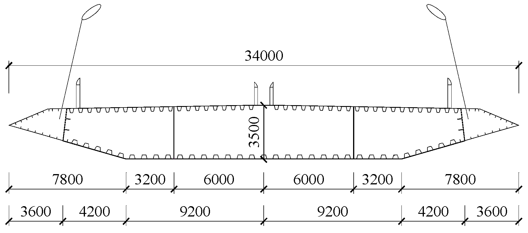
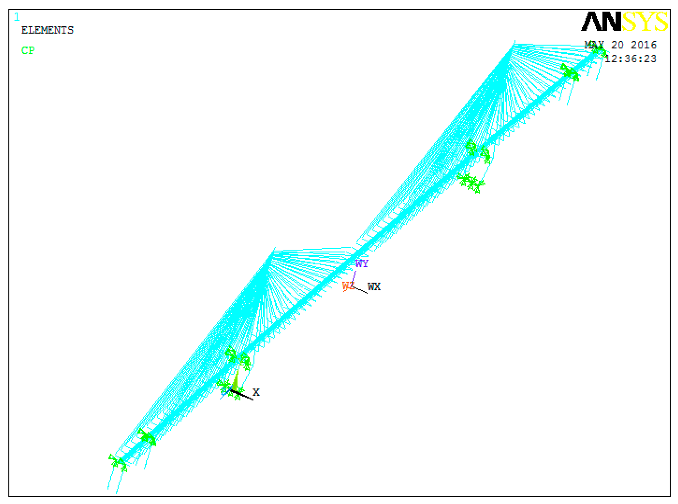
4.1. Finite Element Model of Xiangshan Harbor Bridge

The main bridge of Xiangshan Harbor Bridge in Ningbo City in China is a five-span continuous semi-floating cable-stayed bridge with double towers and double cable planes in Figure 4. The main girder section is a streamlined closed steel box shape, the detailed sizes are marked in Figure 5, and the bridge tower is diamond-shaped. The auxiliary pier and transition pier are rectangular thin-walled types. The foundations of the bridge tower and piers are all bored pile foundations. Vertical and lateral bearings are set between the cable tower and the main beam, and viscous dampers with the function to limit displacement are installed in the longitudinal direction. In this analysis, the limit of dampers on the longitudinal motion of the main beam is ignored, and the main beam is only restrained in the lateral and vertical directions. The longitudinal sliding bearing is set on one side of the transverse bridge direction between the main beam and the transition pier and the auxiliary pier, and the longitudinal sliding bearing on the other side can limit the lateral relative movement at the same time, so it is simplified to constrain the main beam in the lateral and vertical directions, and only coupling the degrees of freedom in the lateral and vertical directions when building the finite element model. And the bottom of the cable tower and piers is consolidated to constrain all degrees of freedom.

The finite element model of Xiangshan Harbor Bridge is established by ANSYS software. This bridge is simulated as a single-ridge girder model as a “fish bone spur” form. The whole modeling process is finished by APDL (ANSYS Parametric Design Language). The main beam, bridge tower, and piers are simulated by BEAM188 element which can give the cross-section shape, the connection between the main girder and stay cables is realized by rigid arms that are modeled by BEAM4 element with high rigidity. The stay cables are modeled by the LINK10 element, and the ballast and the second-stage dead load are substituted by the mass point MASS21 element. The connection between the main beam, the bridge tower, and the pier is simulated by coupling constraint, and the bottom of the bridge tower and bridge piers are consolidated. The complete finite element model of Xiangshan Harbor Bridge is shown in Figure 6.

The dynamic characteristic analysis of this bridge is conducted in accordance with the modal analysis function in ANSYS software, and the natural vibration frequency and mode shape results of the bridge can be extracted. The analysis results of the first ten-order natural vibration frequencies are listed in

Table 1. Modal analysis results of Xiangshan Harbor Bridge.

Number	Calculated Frequency/Hz	Measured Frequency/Hz	Error/%	Mode Shape
1	0.129	——	——	Longitudinal drift of main beam
2	0.206	0.213	2.82	First-order symmetrical lateral bending of main beam
3	0.249	0.250	0.40	First-order symmetrical vertical bending of main beam
4	0.316	0.300	5.33	First-order antisymmetric vertical bending of main beam
5	0.453	0.438	3.20	First-order antisymmetric lateral bending of bridge tower
6	0.457	——	——	First-order symmetrical lateral bending of bridge tower
7	0.482	——	——	Second-order symmetrical vertical bending of main beam
8	0.570	0.525	9.52	First-order antisymmetric lateral bending of main beam
9	0.578	0.600	3.17	Second-order antisymmetric vertical bending of main beam
10	0.628	——	——	Third-order symmetrical vertical bending of main beam

and compared with the measured frequencies of Xiangshan Harbor Bridge by dynamic load tests [21] whose detailed contents are from [28]. It can be found from Table 1 that the difference between the calculated value by the numerical simulation and the measured value by tests is acceptable. Therefore, the established numerical model meets the engineering requirements and can be used for structural response analysis.

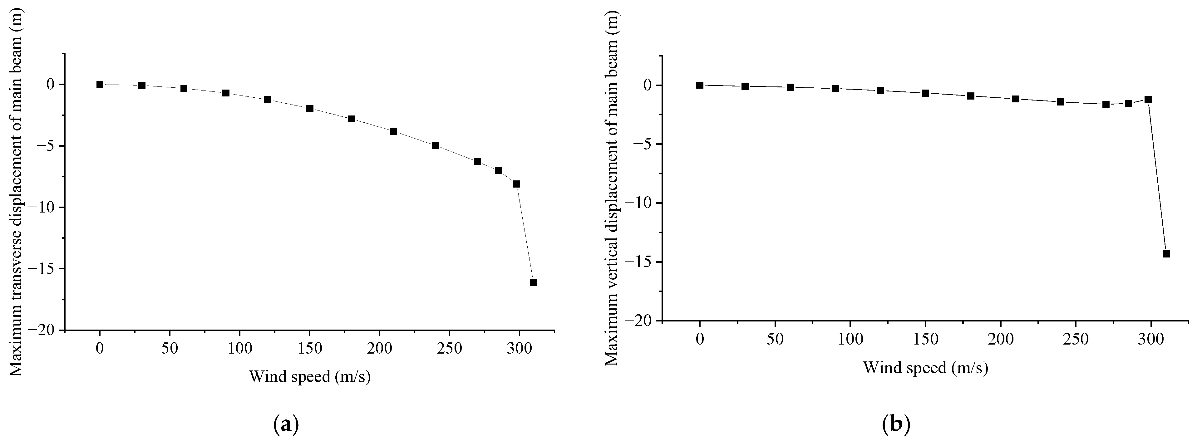
4.2. Calculation of Critical Wind Speed for Static Wind Instability of the Bridge

Combined with the finite element model of the Xiangshan Harbor cable-stayed bridge established in Section 4.1 and the internal and external -two-iterative method for static wind instability analysis of the bridge in Section 2.1.2, the calculation program including three modules which are the information input module (AVINPUT), wind load processing module (WIND_SOLVE) and post-processing module (JUDGE) is written to automatically analyze the static response of the bridge and judge the convergence, the analysis interface is also developed on basis of APDL in ANSYS software. The flow chart of this program is shown in Figure 7.

In the information input module enter the initial wind attack angle and initial wind speed, and initialize the torsion angle of each node of the main beam. In the wind load processing module calculate the wind load on the bridge corresponding to the static wind speed and wind attack angle from the previous module, then solve the displacement of the bridge. And in the post-processing module obtain the torsional displacement of the main beam nodes, take it into the effective wind attack angle and recalculate the corresponding three-component force coefficient, then further calculate the Euclidean norm of each three-component force coefficient and judge whether it is no more than the presupposed allowable value. If it is no more than the allowable value, gradually increase the wind speed and jump to the information input module again, otherwise, the calculated results of the torsion angle of the main girder are added to the effective wind angle of attack, then the calculation is jumped to the wind load processing module.

When calculating the aerostatic instability wind speed, it is necessary to frequently call the information input module, wind load processing module, and post-processing module. But it is time-consuming, inefficient, and very cumbersome to call these modules simply by command flow. Therefore, the above three modules are created as toolbar buttons. When these buttons are clicked, the corresponding module program can be run, thereby realizing the parameterized customization of the toolbar and greatly improving the operating efficiency of the program. After defining the toolbar, the defined toolbar is displayed under the ANSYS Toolbar menu, as shown in Figure 8a. Click the button to realize its corresponding operation, as shown in Figure 8b.

Taking the initial wind angle of attack $\alpha =0°$ as an example, the calculation process of the aerostatic instability wind speed is described. According to the given wind speed solution strategy for static wind instability in Section 2.1.2 and the above program modules, the variation curve of the maximum displacement of the main beam with the wind speed can be plotted, as shown in Figure 9, where it can be seen that the maximum displacement of the main beam increases nonlinearly with the increasing wind speed. When it is close to the instability wind speed, the displacement increases sharply, and the instability wind speed can be inferred according to the changing trend of the displacement. When the initial wind angle of attack $\alpha =0°$, the instability wind speed is 298 m/s, which is unlikely to reach in a practical environment. However, for some bridges, the wind speed of aerostatic instability is much smaller, and the static wind stability even becomes the limiting factor of bridge wind-resistant design. Some examples are given in Ref. [5]. Therefore, this paper provides a method for static wind instability analysis, which can be used for all bridges. Of course, due to the limitations of software and models, some factors such as strength failure are temporarily ignored, where such high wind speed may have caused static failure to the bridge structure.

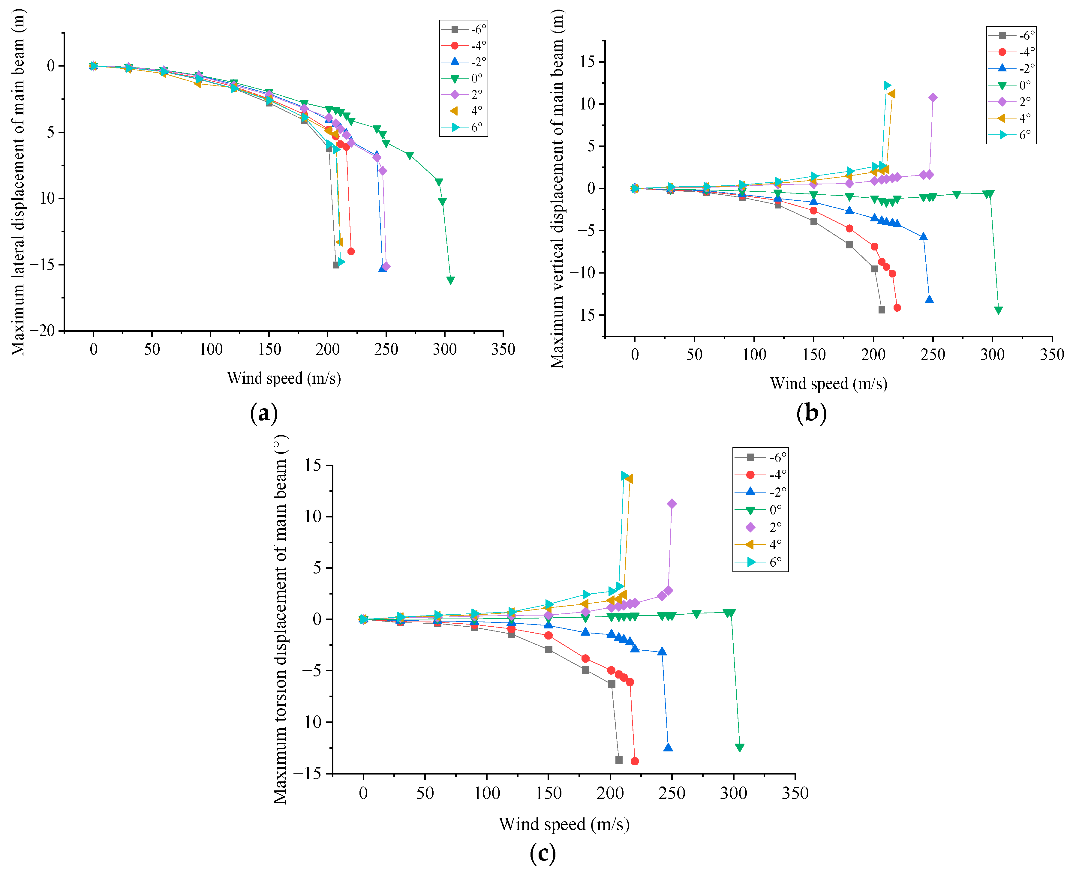
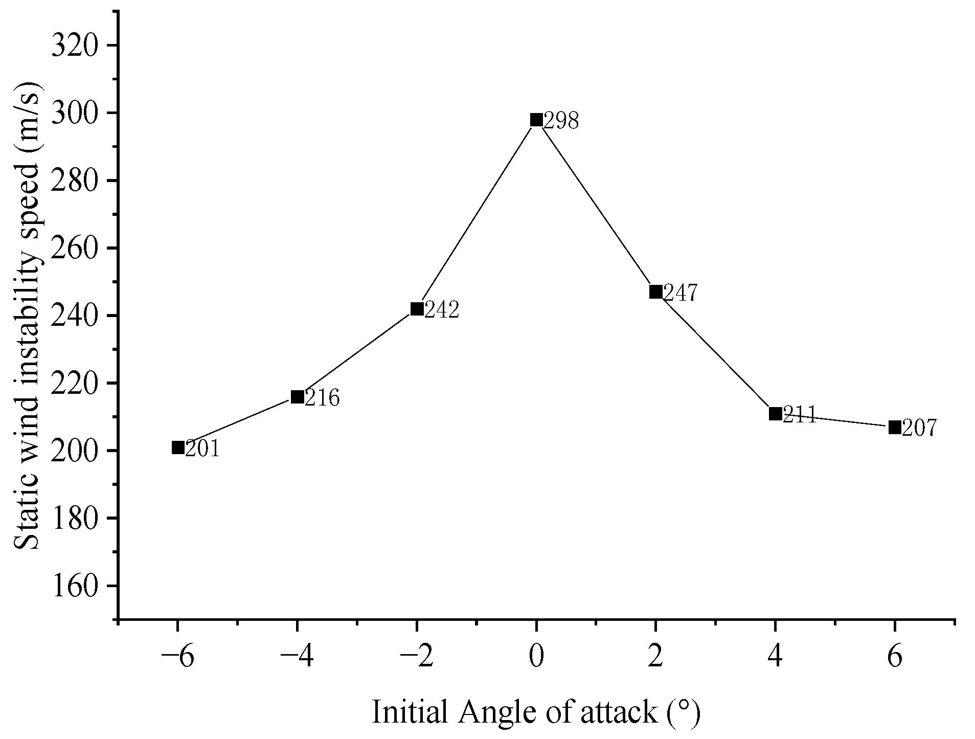
4.3. Influence of Initial Wind Attack Angle on Static Wind Stability

The aerostatic instability wind speed when the initial wind angle of attack $\alpha =0°$ is given above, but in engineering practice, the angle of attack between the incoming wind and the bridge is not necessarily $0°$. And the wind angle of attack is an important factor affecting the critical instability wind speed because the three-component force coefficient for calculating wind load is closely related to the wind angle of attack from Figure 2 where it can be seen that the three-component force coefficient is very different under different wind attack angles. In summary, it is necessary to study the influence of the initial wind angle of attack on static wind stability. There are some studies about the range of initial wind attack angles. He [29] pointed out that the wind angle of attack in the atmospheric boundary layer may vary slightly at the range of −3° to 3°. Han [23] selected the initial wind attack angles as −2°, −1°, 0°, 1°, 2°, and 3° to calculate and compare the critical wind speed for static wind instability of the Second Yangtze River Bridge in Fengdu. To discuss the impact of the initial wind angle of attack more deeply, in this research the initial angle of attack as −6°, −4°, −2°, 0°, 2°, 4°, and 6° are chosen to calculate the aerostatic instability wind speed, respectively.

Then the displacement response curves of the bridge can be plotted considering different wind attack angles and wind speeds in Figure 10. From the analysis results of static wind instability, it can be seen that the static wind instability form of Xiangshan Harbor Bridge is a flexure-torsion coupling type. And the critical instability wind speed under different initial wind attack angles can be inferred from the displacement response curves, plotted in Figure 11. While the initial wind angle of attack varies from −6° to 6°, the critical instability wind speed first increases nonlinearly and reaches the maximum value at 0°; then it decreases nonlinearly. The maximum and minimum critical instability wind speeds are 298 m/s and 201 m/s, respectively.

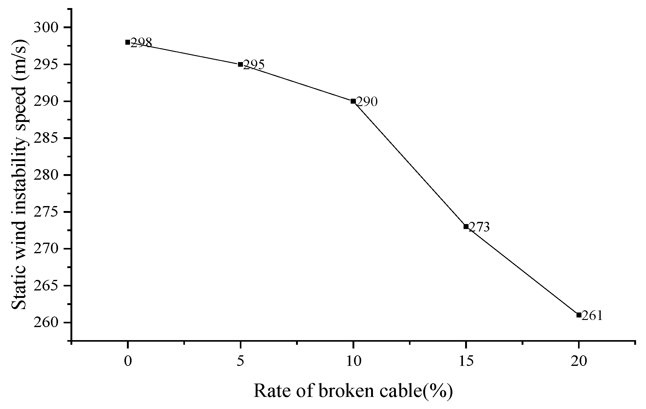
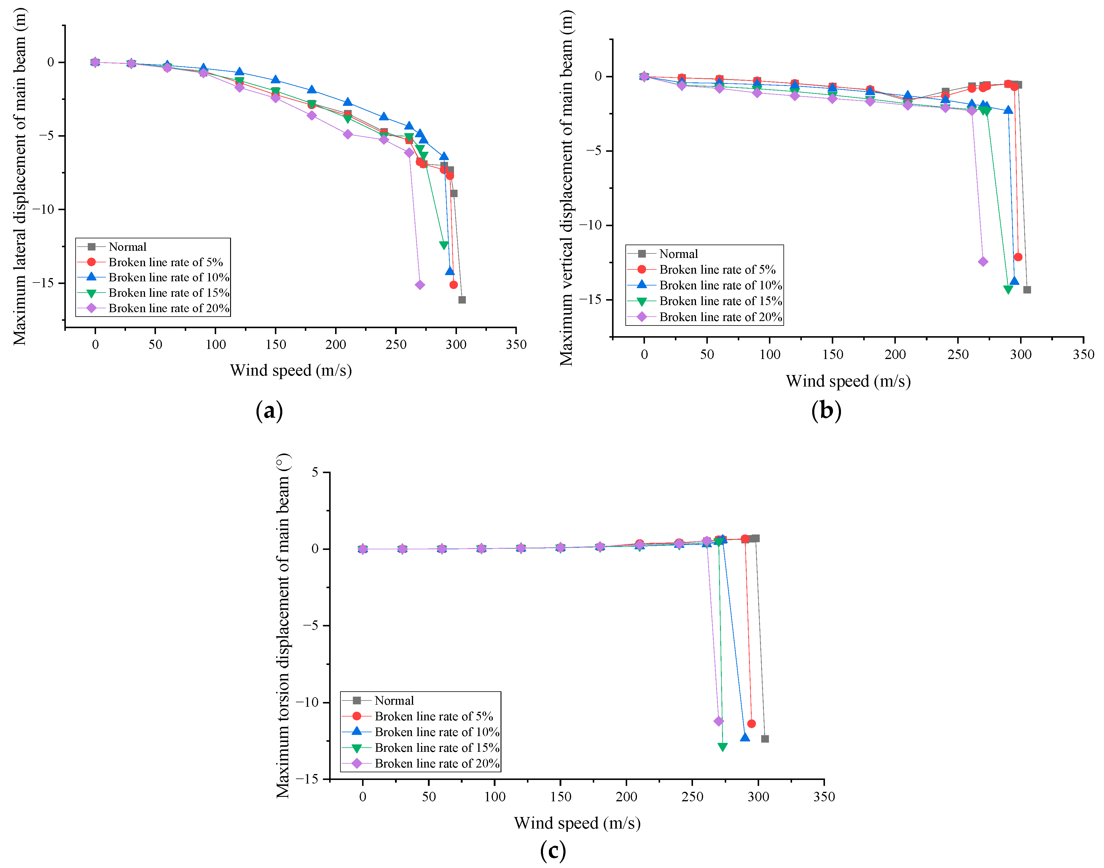
4.4. Influence of Steel Wire Breakage Rate in Stay Cables on Static Wind Stability

During the long-term service of long-span cable-stayed bridges, steel wire of stay cables may break due to environmental impact and load action, which will lead to the redistribution of cable stress because of the cross-sectional area decrease of the stay cable and reduce the safety performance of the bridge. Lan [30] pointed out through experimental research that the steel wire breakage rate doesn’t exceed 10% otherwise the stay cable should be replaced. For the purpose of exploring the influence of the steel wire breakage rate on the static wind stability of the bridge, 5%, 10%, 15%, and 20% steel wire breakage rates are considered by changing the sectional area of the stay cables. Then the displacement response of Xiangshan Harbor Bridge is calculated and compared under the different steel wire breakage rates. The maximum displacement of the main beam in Xiangshan Harbor Bridge is plotted in Figure 12. Further, the critical aerostatic instability wind speed of the bridge under different steel wire breakage rates can be inferred from the displacement response curves, as shown in Figure 13.

From the results in the above figure, when the steel wire breakage rate is less than 10%, it has little effect on the static wind instability, but more than 10%, the critical instability wind speed of the bridge decreases rapidly. When the steel wire breakage rate is 20%, the critical instability wind speed is 261 m/s, which is 12% lower than before. Therefore, the stay cables should be inspected regularly, and the broken wire shall be replaced in time during the operation stage of the bridge.

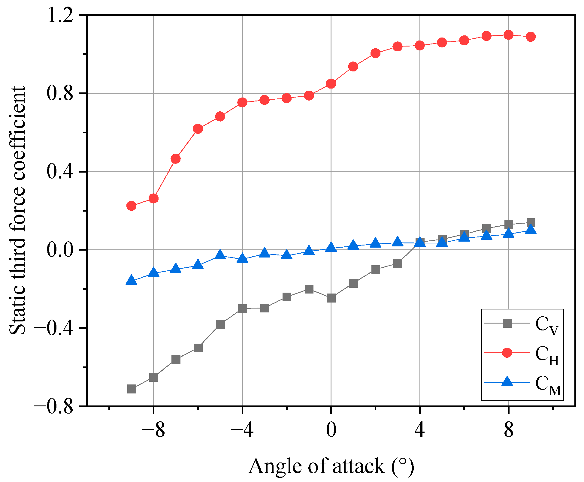
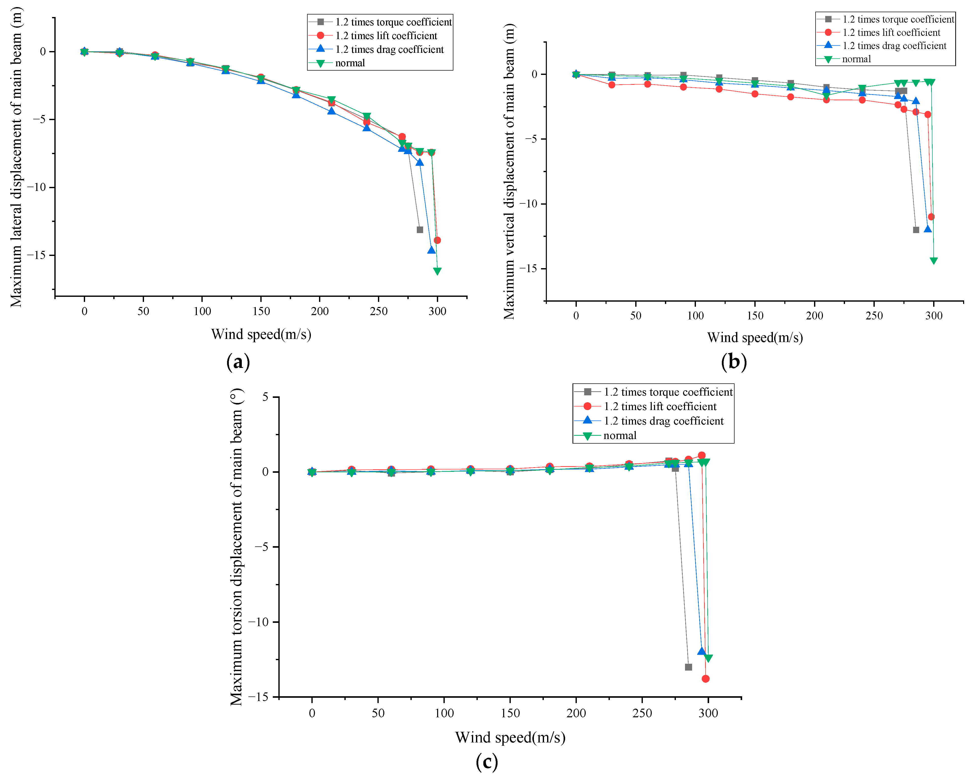
4.5. Influence of Static Three-Component Force Coefficients on Static Wind Stability

Due to the randomness of the wind field and the fluid-structure interaction during the use of the bridge, the magnitude of the static three-component force coefficient will also fluctuate accordingly. These coefficients obtained by boundary layer wind tunnel test or numerical simulation also are random. It is very important for the static wind load calculation, and the static wind load is closely related to the static wind instability of the bridge. Therefore, it is necessary to discuss the sensitivity of the static three-component force coefficient to the static wind instability of the bridge. In this research, the static wind stability of the Xiangshan Harbor Bridge is respectively explored when only the moment coefficient is expanded to 1.2 times, and other parameters remain unchanged, or only the lift coefficient is expanded to 1.2 times, or only the drag coefficient is expanded to 1.2 times, to analyze the displacement response of the bridge and obtain the critical instability wind speed. The comparison of the maximum displacement of the main beam under different cases is shown in Figure 14. The critical instability wind speed of Xiangshan Harbor Bridge under different cases is listed in

Table 2. Static instability wind speeds under different three-component force coefficients.

Item	Normal	1.2 Times Moment Coefficient	1.2 Times Lift Coefficient	1.2 Times Drag Coefficient
Static wind instability speed (m/s)	298	275	295	285

at the initial wind attack angle of 0°.

From the above results, it can be concluded that the change in the moment coefficient has the greatest influence on the static wind stability, and the change in the lift coefficient has a great influence on the vertical displacement of the bridge but it has little effect on the aerostatic instability wind speed.

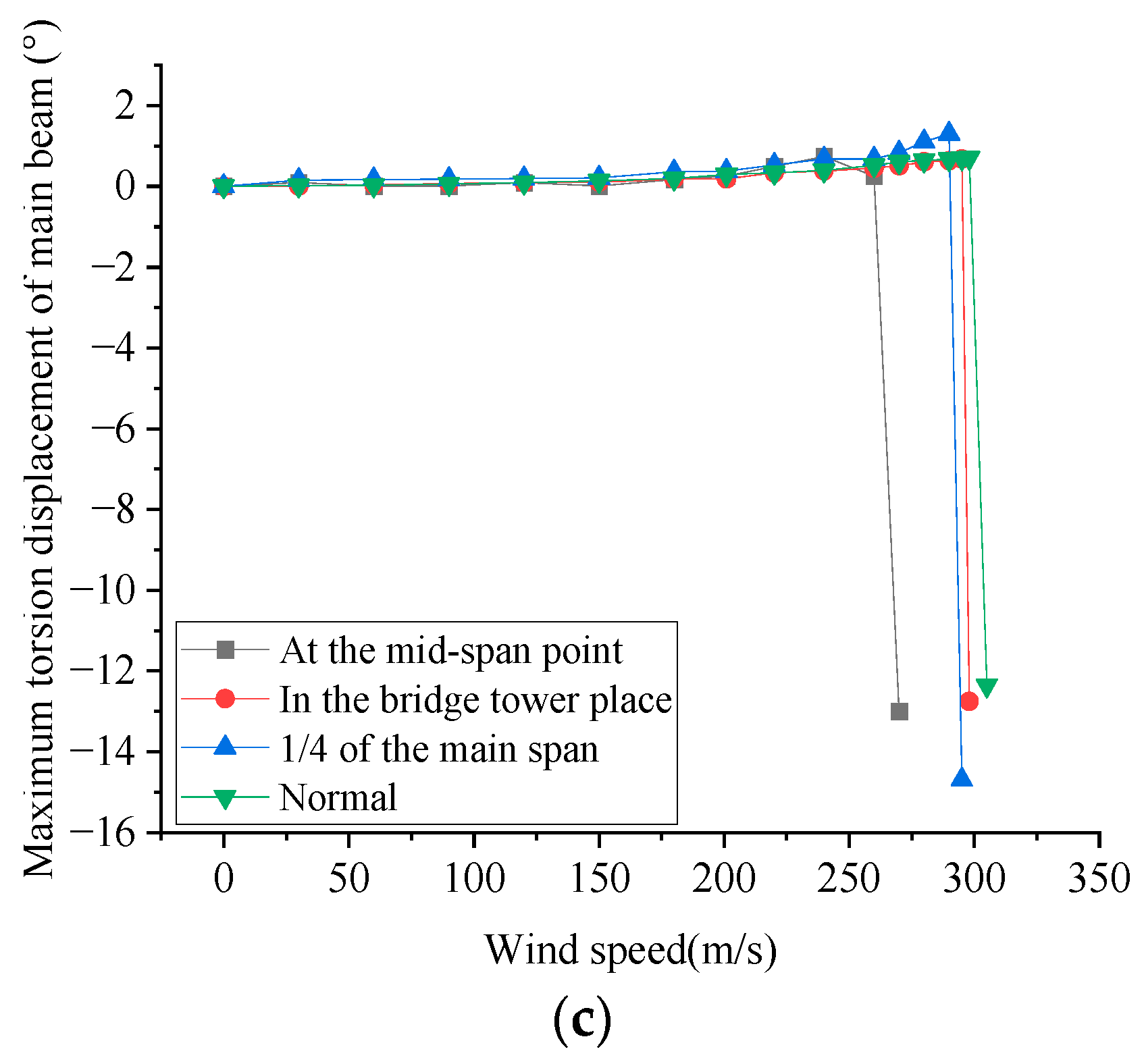
4.6. Influence of Stay Cable Broken Position on Static Wind Stability

During the use of the bridge, the stay cable will lose its function entirely (or called stay cable broken) due to the occurrence of some special circumstances or replacement of stay cables. To discuss the influence of the stay cable broken position on static wind stability, there are three cases about the broken position of the stay cable, that is, the stay cable breaks in the middle position of the main span, in the quarter position of the main span and near to the bridge tower, and they are called Condition 1, Condition 2 and Condition 3, as shown in Figure 15. The comparison of the maximum displacement of the main beam under different conditions is shown in Figure 16. The critical instability wind speed of Xiangshan Harbor Bridge under different conditions is listed in

Table 3. Aerostatic instability wind speeds under different broken positions of the stay cable.

Cable Broken Position	Normal	Condition 1	Condition 2	Condition 3
Static wind instability speed (m/s)	298	260	290	295

at the initial wind attack angle of 0°.

From the above results, three broken positions of the stay cable are analyzed to get the aerostatic instability wind speeds of Xiangshan Harbor Bridge are 260 m/s, 295 m/s, and 290 m/s, respectively. It is proved that the broken stay cables near the main tower have almost no effect on the critical aerostatic instability wind speed, but the influence of stay cable breakage in mid-span is great, which makes the aerostatic instability wind speed decrease by 12.8%.

5. Analysis of Static Wind Reliability for Xiangshan Harbor Bridge

5.1. Calculation of Static Wind Reliability

For the cable-stayed bridges in service, the factors that affect the static wind stability are essentially stiffness and static wind load, where the main forms of expression are the change of the static three-component force coefficient, the rupture of the stay cables, the change of the stiffness of the main beam, the change of the constraint, etc. Combined with the parameter influence analysis of the static wind stability for Xiangshan Harbor Bridge in Section 4.1, it can be found that the influence of moment coefficient, stay cable broken position and steel wire breakage rate in stay cables cannot be ignored, and among these parameters, the moment coefficient, steel wire breakage rate in stay cables and stay cable broken position have random characteristics and important effects on the static wind stability of the bridge, so these three parameters are taken as random variables in the static wind reliability analysis of Xiangshan Harbor Bridge. The steel wire breakage rate is taken as 20% for static wind reliability analysis, so the design value of the sectional area of the stay cable is 0.20085 m², and its variation coefficient is taken as 0.05 according to relevant papers on bridge reliability calculation and suggestions in Uniform Standard for Reliability Design of Engineering Structures (GB 50153-2008) [31]_. For the moment coefficient of the main girder, the design value is shown in Figure 2, and the variation coefficient of the aerodynamic force coefficient of the main girder from the boundary layer wind tunnel test is usually around 0.15 according to previous research [32], so the variation coefficient of the moment coefficient is taken as 0.15. But there is no corresponding standard for the value of the stay cable broken location, the design value is taken as 5 considering the project practice, and the variation coefficient is taken as 0.5. These three random parameters and their distribution are listed in

Table 4. Parameter distribution and statistical characteristic values.

Random Parameters	Distribution Type	Average Value	Variation Coefficient
Moment coefficient	Normal distribution	1.00	0.15
Cross-sectional area of stay cable	Normal distribution	1.00	0.05
Stay cable broken position	Normal distribution	1.00	0.50

Note: Average value represents the ratio of actual value to design value; In practice, the steel wire breakage rate in stay cables is simulated by changing the sectional area of the stay cable; About the stay cable broken position, the length between the mid-span of the bridge and the main tower is divided into ten equal parts, the stay cable broken position is obtained by the design value 5 multiplying by the sample value, if the calculated result is negative or more than 10, the stay cable broken position shall be the nearest to the main tower.

.

Based on the theory in Section 2.2, the LHS method is used to sample these parameters 30 times in MATLAB 2020b, listed in

Table 5. Results of LHS for 30 times for different parameters.

Sample No.	Moment Coefficient	Steel Wire Breakage Rate	Stay Cable Broken Position
1	0.920728	0.949115	1.082463
2	0.974271	1.041689	0.981851
3	0.771126	1.061711	0.746454
4	1.287531	1.095844	0.908971
5	1.254599	0.966521	2.168303
6	0.961617	1.005954	0.929463
7	0.934908	0.999166	1.598472
8	1.079174	0.979184	1.478054
9	0.997497	0.973576	1.338008
10	0.980966	1.024584	0.281436
11	1.017861	0.959554	1.110001
12	1.048353	1.000593	0.204652
13	0.847346	1.067997	1.128450
14	1.106737	0.987206	1.405852
15	0.856827	0.993655	1.243036
16	1.036913	1.021351	0.374567
17	1.001778	1.084866	0.545285
18	1.125068	0.923709	0.866323
19	1.064053	0.991424	0.596021
20	0.779631	1.046271	1.492150
21	1.161102	0.943786	0.514781
22	1.185132	1.053701	1.733024
23	0.831357	1.012304	1.883946
24	1.138812	0.903784	0.659194
25	1.203990	1.026391	1.181329
26	0.878663	1.035579	-0.089507
27	1.073751	0.959554	0.820229
28	0.711353	0.952276	1.285940
29	0.899563	0.926544	1.011250
30	0.937552	1.016118	1.046224

. When analyzing static wind stability, the specific value of each parameter is equal to the design value multiplied by the sampling value in Table 5, then these specific values are input into analysis modules for the deterministic analysis of static wind instability of the bridge in Section 4.2 to obtain the critical aerostatic instability wind speed. During the calculation process, if one parameter takes the sampling value, other parameters take the design value. The 30 groups of instability wind speeds for every random parameter are given in

Table 6. Aerostatic instability wind speeds corresponding to 30 samples for different parameters (m/s).

Sample No.	Moment Coefficient	Steel Wire Breakage Rate	Stay Cable Broken Position
1	304	257	278
2	301	263	260
3	316	265	282
4	277	267	280
5	282	259	298
6	301	261	269
7	303	261	290
8	292	260	290
9	298	259	286
10	299	262	295
11	297	259	279
12	295	261	293
13	309	265	280
14	291	260	290
15	308	260	281
16	296	262	290
17	298	266	290
18	289	255	280
19	294	260	287
20	313	264	290
21	287	257	290
22	286	264	292
23	311	262	293
24	288	254	285
25	282	263	281
26	307	263	298
27	293	258	281
28	318	258	283
29	306	256	260
30	303	262	264

, and the statistic characteristic values of the critical aerostatic instability wind speed are summarized in

Table 7. Statistic characteristic values of wind speed for static wind instability.

Static Wind Instability Speed (m/s)	Moment Coefficient	Steel Wire Breakage Rate	Stay Cable Broken Position
Mean value	298	260	284
Standard deviation	10.18	3.16	9.67

.

According to the calculation results in the above table, the mean value and standard deviation of aerostatic instability wind speed under three conditions can be obtained, then the corresponding probability distribution parameters are substituted into the reliability calculation formulas respectively, and the reliability index of the above three conditions can be obtained. Because the functional function is $Z=C_w{U}_s-G_v{U}_b$, the limit state is $Z=C_w{U}_s-G_v{U}_b=0$. The reliability index is calculated by the checkpoint method, for convenience, the functional function is also denoted as $g\left(x\right)=X_1{X}_2-X_3{X}_4$, and its gradient function is denoted as $gX=\left(X_2,X_1,-X_4,-X_3\right)$. The reliability indexes and the values of checkpoints are given in

Table 8. Calculation results of static wind reliability.

Item	Moment Coefficient	Steel Wire Breakage Rate	Stay Cable Broken Position
Reliability index	6.3375	5.9757	6.1908
$C_w$	0.7500	0.7753	0.7613
$U_s$	291.5469	260.4271	277.5833
$G_v$	1.6144	1.6003	1.6083
$U_b$	135.4469	126.1683	131.4031

.

5.2. Static Wind Reliability under Different Conditions

During the whole life cycle of a bridge, various situations that are unfavorable to the wind stability of the bridge will inevitably occur, such as the steel wire breakage of stay cables or even a whole stay cable breaking. On basis of the above static wind reliability analysis, the same method is used for the static wind reliability under different mean values of steel wire breakage rates and the different stay cable broken positions.

For different steel wire breakage rates of stay cables, the variation coefficient of the critical wind speed for static wind instability is 0.014. On this basis, supplementary deterministic analysis is carried out on the 0%, 5%, 10%, and 15% steel wire breakage rates, then the reliability index can be obtained similar to the method in Section 5.1, and the reliability index is transformed into the corresponding failure probability. They are given in

Table 9. Static wind instability probability corresponding to different steel wire breakage rates.

Steel Wire Breakage Rate	0%	5%	10%	15%	20%
Reliability index	6.3645	6.3344	6.2836	6.1050	5.9757
Failure probability	9.795 × 10−11	1.199 × 10−10	1.654 × 10−10	5.133 × 10−10	1.145 × 10−9

. It can be seen from Table 9 that the reliability index gradually decreases with the increase of steel wire breakage rate, but in general, the static wind failure probability of Xiangshan Harbor Bridge is very low, so there is no static wind instability problem.

For different stay cable broken positions, the variation coefficient of the critical wind speed for static wind instability is 0.034. On this basis, supplementary deterministic analysis is conducted when the broken stay cable is close to the main tower, at mid-span, and 1/4 of the main span. Similarly, the reliability index can be obtained and it can be transformed into the corresponding failure probability, which is listed in

Table 10. Static wind instability probability corresponding to different broken cable positions.

Stay Cable Broken Position	Random Location	Near to Bridge Tower	1/4 of the Main Span	1/2 of the Main Span
Reliability index	6.1908	6.3063	6.2559	5.9371
Failure probability	2.993 × 10−10	1.429 × 10−10	1.976 × 10−10	1.450 × 10−9

.

6. Conclusions

In this paper, taking the existing Xiangshan Harbor cable-stayed bridge as the background, the finite element model established by ANSYS 15.0 software is used to solve the aerostatic instability of wind speed. At the same time, the parameter impact analysis is discussed, and the static wind reliability calculation is conducted to obtain the static wind reliability index of the cable-stayed bridge. There are some conclusions as follows:

(1)

According to the results for the static wind stability of Xiangshan Harbor Bridge at the initial wind angle of attack $\alpha =0°$, it is found that the static wind instability mode for Xiangshan Harbor Bridge is bending-torsional coupling instability, and the critical wind speed of static wind instability is the highest when the initial wind attack angle is 0°, the aerostatic instability wind speed of the bridge commonly reduces with the increase of the initial wind angle of attack. So other wind attack angles shall also be analyzed in the bridge design besides the 0° wind attack angle.

(2)

The aerostatic instability wind speed does not vary obviously with the change of the steel wire breakage rate of the stay cables, but it is necessary to closely monitor the situation that the steel wire breakage rate of the stay cable exceeds 10%. The aerodynamic drag coefficient and moment coefficient of the main girder play a more important role than the lift coefficient in causing static wind instability. And the stay cable broken position has a great impact on the static wind stability of the bridge structure, especially when the broken cables locating at the mid-span of the main beam, the wind environment should be closely monitored when replacing the stay cables.

(3)

The uncertainty analysis of static wind instability for the bridge is conducted by combining the LHS method and the checking point method. The uncertain influence of three key parameters including moment coefficient, steel wire breakage rate, and the stay cable broken position is considered for Xiangshan Harbor Bridge in service. Then the static wind reliability indexes are obtained when these three key parameters are taken as random variables, respectively, which are 6.3375, 5.9757, and 6.1908. The static wind reliability of Xiangshan Harbor Bridge is very high.

(4)

The static wind reliability indexes of Xiangshan Harbor Bridge in service under different steel wire breakage rates and different cable broken positions are compared. It is found that the most unfavorable situation is that the steel wire breakage rate is 20% and the broken position of the stay cable is at the midspan of the main beam, the reliability index is 5.9757 and 5.9371, respectively. But corresponding to these two unfavorable conditions the order of magnitude of failure probability is 10⁻⁹, which also proves that the static wind stability of Xiangshan Harbor Bridge is very good.

References

1. Ge, Y.J. Aerodynamic challenge and limitation in long-span cable-supported bridges. In Proceedings of the 2016 World Congress on Advances in Civil, Environmental, and Materials Research, Jeju island, Republic of Korea, 28 August–1 September 2016. [Google Scholar]
2. Simiu, E.; Scanlan, R.H. Wind Effects on Structures: An Introduction to Wind Engineering; John Wiley & Sons Inc.: New York, NY, USA, 1978. [Google Scholar]
3. Scanlan, R.H. The action of flexible bridges under wind, I: Flutter theory. J. Sound Vib. 1978, 60, 187–199. [Google Scholar] [CrossRef]
4. Larsen, A.; Larose, G.L. Dynamic wind effects on suspension and cable-stayed bridges. J. Sound Vib. 2015, 334, 2–28. [Google Scholar] [CrossRef]
5. Montoya, M.C.; Hernández, S.; Kareem, A.; Nieto, F. Efficient modal-based method for analyzing nonlinear aerostatic stability of long-span bridges. Eng. Struct. 2021, 244, 112556. [Google Scholar] [CrossRef]
6. Shao, G.P.; Gong, J.C.; Liu, M.W. Analysis of nonlinear static wind effect of long-span suspension bridge. Sichuan Archit. 2020, 40, 329–332. [Google Scholar]
7. Hirai, A.; Okauchi, I.; Ito, M.; Miyata, T. Studies on the critical wind velocity for suspension bridges. In Proceedings of the International Research Seminar on Wind Effects on Buildings and Structures, Ottawa, ON, Canada, 11–15 September 1967; Volume 2, pp. 81–103. [Google Scholar]
8. Cheng, J. Study on Nonlinear Aerostatic Stability of Cable-Supported Bridges. Ph.D. Thesis, Tongji University, Shanghai, China, 2000. [Google Scholar]
9. Cheng, J.; Jiang, J.J.; Xiao, R.C.; Xiang, H.F. Nonlinear aerostatic stability analysis of Jiang Yin suspension bridge. Eng. Struct. 2002, 24, 773–781. [Google Scholar] [CrossRef]
10. Boonyapinyo, V.; Yamada, H.; Miyata, T. Wind-induced nonlinear lateral-torsional buckling of cable-stayed bridges. J. Struct. Eng. 1994, 120, 486–506. Available online: https://ascelibrary.org/doi/abs/10.1061/(ASCE)0733-9445(1994)120:2(486) (accessed on 1 May 2021). [CrossRef]
11. Boonyapinyo, V.; Lauhatanon, Y.; Lukkunaprasit, P. Nonlinear aerostatic stability analysis of suspension bridges. Eng. Struct. 2006, 28, 793–803. [Google Scholar] [CrossRef]
12. Nagai, M.; Xie, X.; Yamaguchi, H.; Fujino, Y. Static and dynamic instability analyses of 1400-meter long-span cable-stayed bridges. In IABSE Symposium Reports; International Association for Bridge and Structural Engineering (IABSE): Kobe, Japan, 1998; Volume 9, pp. 281–286. [Google Scholar]
13. Cheng, J.; Jiang, J.J.; Xiao, R.C. Aerostatic stability analysis of suspension bridges under parametric uncertainty. Eng. Struct. 2003, 5, 1675–1684. [Google Scholar] [CrossRef]
14. Zhou, Q.; Zhou, Z.Y.; Ge, Y.J. Mode and mechanism of aerostatic stability for suspension bridges with double main spans. J. Harbin Inst. Technol. 2012, 44, 76–82. [Google Scholar]
15. Su, C.; Luo, X.F.; Yun, T.Q. Aerostatic reliability analysis of long-span bridges. J. Bridge Eng. 2010, 15, 260–268. [Google Scholar] [CrossRef]
16. Li, J.W.; Fang, C.; Hou, L.M.; Wang, J. Sensitivity analysis of static wind stability parameters of long-span bridges. J. Vib. Shock. 2014, 33, 124–130. [Google Scholar]
17. Imai, K.; Frangopol, D.M. Geometrically nonlinear finite element reliability analysis of structural systems. I: Theory. Comput. Struct. 2000, 77, 677–691. [Google Scholar] [CrossRef]
18. Frangopol, D.M.; Imai, K. Geometrically nonlinear finite element reliability analysis of structural systems. II: Applications. Comput. Struct. 2000, 77, 693–709. [Google Scholar] [CrossRef]
19. Chen, W.Z.; Tang, T.; Xu, J. Cable-stayed bridge structural system reliability assessment theory research progress. J. Bridge Constr. 2006, 4, 67–70. [Google Scholar]
20. Liang, H.L. Reliability Analysis of Static Wind Instability of Steel Truss Pedestrian Suspension Bridge. Ph.D. Thesis, Xi’an University of Science and Technology, Xi’an, China, 2018. [Google Scholar]
21. Xu, Y.L. Wind Effects on Cable-Supported Bridges; Wiley: New York, NY, USA, 2013. [Google Scholar]
22. JTG/T 3360-01-2018; Wind-Resistant Design Specification for Highway Bridges. China Communications Press: Beijing, China, 2017.
23. Han, D.J.; Zou, X.J. Analysis of nonlinear static wind stability of long-span cable-stayed bridge. Eng. Mech. 2005, 22, 206–210. [Google Scholar]
24. Ditlevsen, O.; Madsen, H.O. Structural Reliability Methods, 2nd ed.; Wiley: New York, NY, USA, 2007. [Google Scholar]
25. Bao, J.W.; Hu, X.Y.; Xing, M.Y.; Zhao, S.F. Comparative study of latin hypercube and traditional selective sampling in reliability analysis. J. North China Univ. Sci. Technol. 2021, 18, 81–84. [Google Scholar]
26. China Meteorological Data Net/National Meteorological Science Data Center. Available online: http://data.cma.cn/ (accessed on 27 April 2017).
27. Zhang, T.; Cui, X.J.; Zhang, X.F.; Li, H.J.; Zou, Y.F. Flutter Reliability Analysis of Xiangshan Harbor Highway Cable-Stayed Bridges in Service. Appl. Sci. 2022, 12, 8301. [Google Scholar] [CrossRef]
28. Tang, J.L.; Xu, J.H. Load Test Report of the Main Bridge of Xiangshan Harbor Bridge; Zhejiang Jiaoke Engineering Inspection Co., Ltd.: Hangzhou, China, 2012; Volume 24–27, pp. 94–99. [Google Scholar]
29. He, H.X. The Analysis and Research on the Bridge’s Seismic Resistance, Wind Resistance and Their Influence Factors. Ph.D. Thesis, Chang’an University, Xi’an, China, 2011. [Google Scholar]
30. Lan, C.M. Theoretical study on fatigue performance of parallel steel cable. J. Shenyang Jianzhu Univ. Nat. Sci. 2009, 25, 56–60. [Google Scholar]
31. GB 50153-2008; Unified Standard for Reliability Design of Engineering Structures. China Architecture Press: Beijing, China, 2008.
32. Liu, Z.W. Wind-Resistant Risk Assessment of Cable-Supported Bridges. Ph.D. Thesis, Tongji University, Shanghai, China, 2004. [Google Scholar]
Figure 1. Three-component force on the girder section in the body axis coordinate system.
Applsci 13 00749 g001
Figure 2. Aerodynamic force coefficient of the main girder of Xiangshan Harbor Bridge in body axis coordinate system.
Applsci 13 00749 g002
Figure 3. Calculation flow chart of checkpoint method for reliability analysis.
Applsci 13 00749 g003
Figure 4. Layout of main bridge (m).
Applsci 13 00749 g004
Figure 5. Cross-section layout of steel box girder (mm).
Applsci 13 00749 g005
Figure 6. Finite element model of Xiangshan Harbor Bridge.
Applsci 13 00749 g006
Figure 7. Flowchart of the static wind instability solution program.
Applsci 13 00749 g007
Figure 8. ANSYS solution process diagram. (a) User Toolbar; (b) Parameter input dialog box.
Applsci 13 00749 g008
Figure 9. Variation curves of the maximum displacement of the main beam with wind speed. (a) Transverse displacement; (b) Vertical displacement; (c) Torsion angle.
Applsci 13 00749 g009aApplsci 13 00749 g009b
Figure 10. Maximum displacement curve of the main beam with wind speed under different initial wind attack angles; (a) Lateral displacement (b) Vertical displacement; (c) Torsion angle.
Applsci 13 00749 g010
Figure 11. Variation curve of critical instability wind speed with the initial wind angle of attack.
Applsci 13 00749 g011
Figure 12. Maximum displacement curve of main beam with wind speed under different wire breakage rates; (a) Lateral displacement (b) Vertical displacement; (c) Torsion angle.
Applsci 13 00749 g012
Figure 13. Critical aerostatic instability wind speed with the steel wire breakage rate.
Applsci 13 00749 g013
Figure 14. Maximum displacement curve of main beam with wind speed under different three-component force coefficients; (a) Lateral displacement; (b) Vertical displacement; (c) Torsion angle.
Applsci 13 00749 g014
Figure 15. Stay cable broken position (m).
Applsci 13 00749 g015
Figure 16. Maximum displacement curve of main beam with wind speed under different broken positions of the stay cable; (a) Lateral displacement; (b) Vertical displacement; (c) Torsion angle.
Applsci 13 00749 g016aApplsci 13 00749 g016b