

Experimental and Modeling Investigation for Slugging Pressure under Zero Net Liquid Flow in Underwater Compressed Gas Energy Storage Systems
 ,
,  ,
, 

Abstract
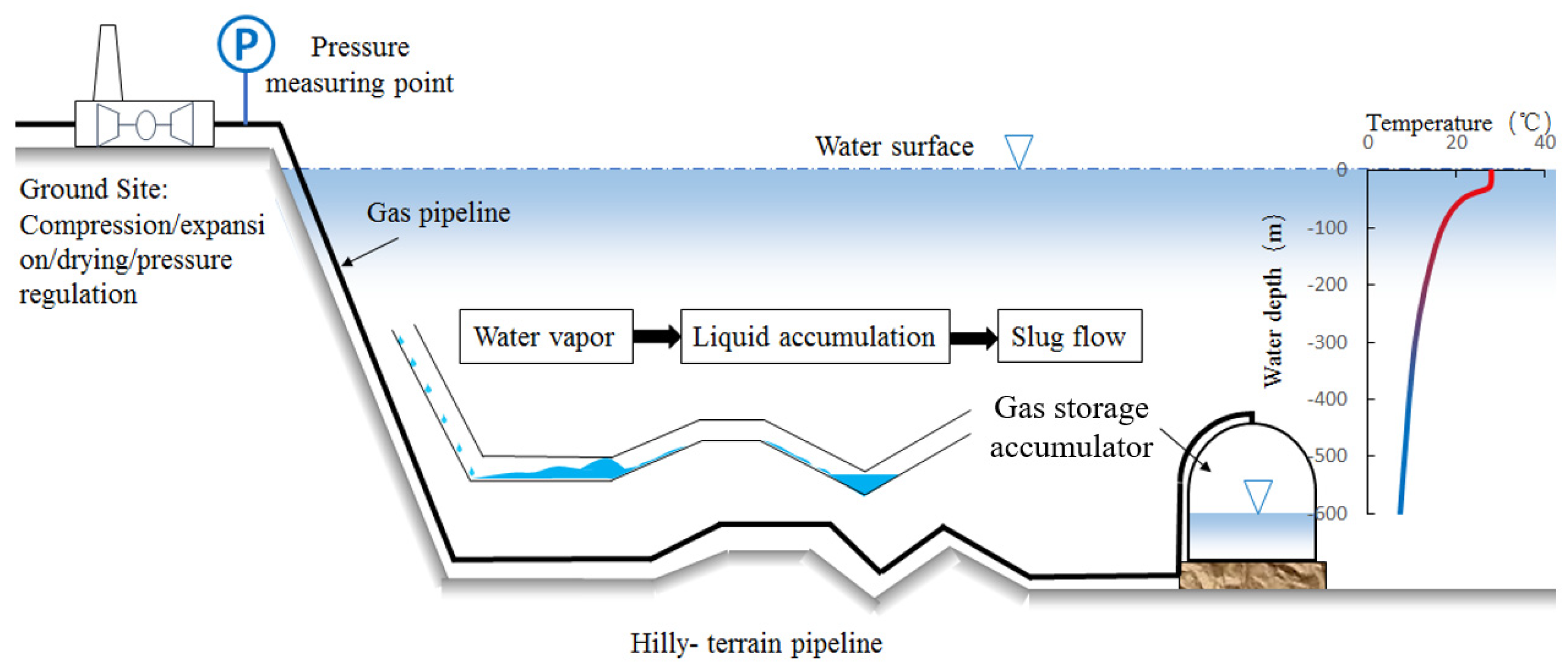
1. Introduction
2. Experiment
2.1. Test Rig and Measurement Details
2.2. Experimental Procedure
3. Modeling
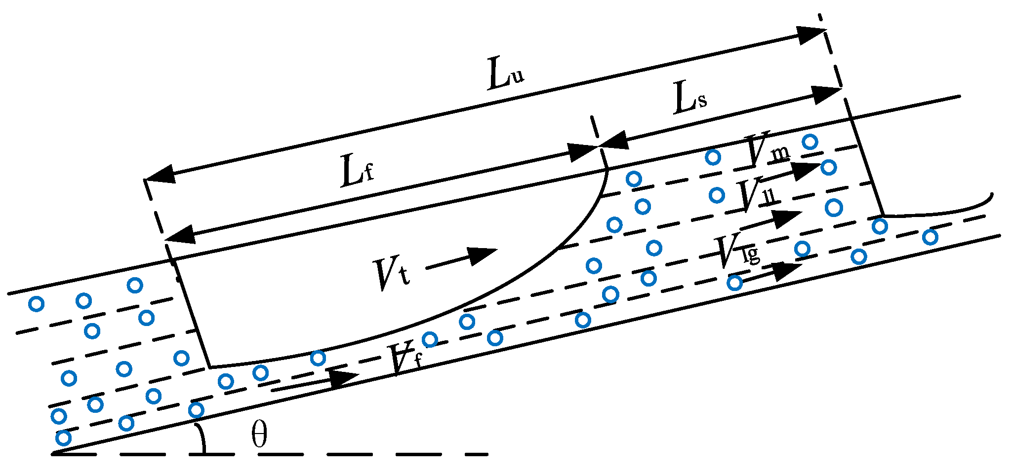
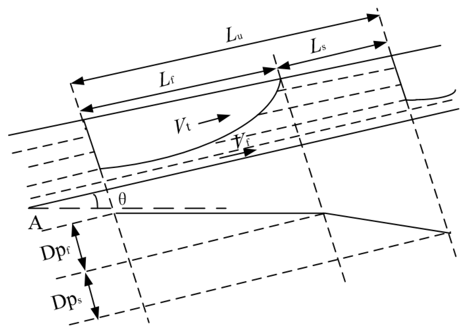
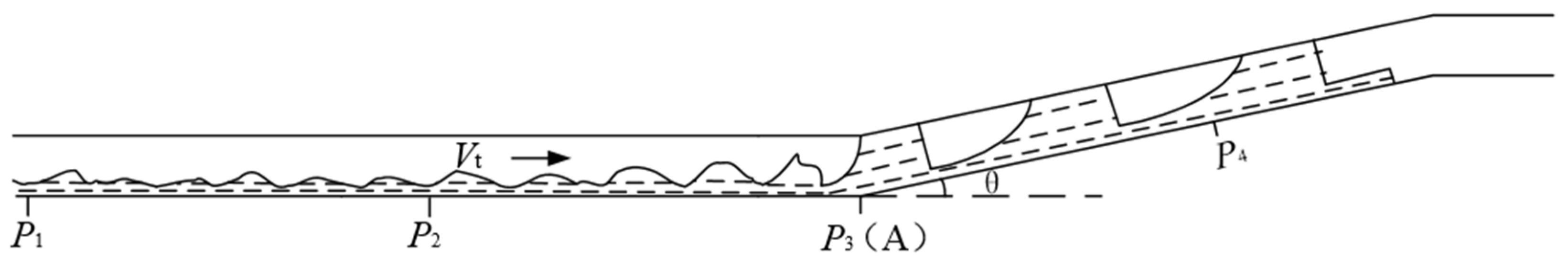
3.1. Slug Unit Pressure Model in Inclined Pipe
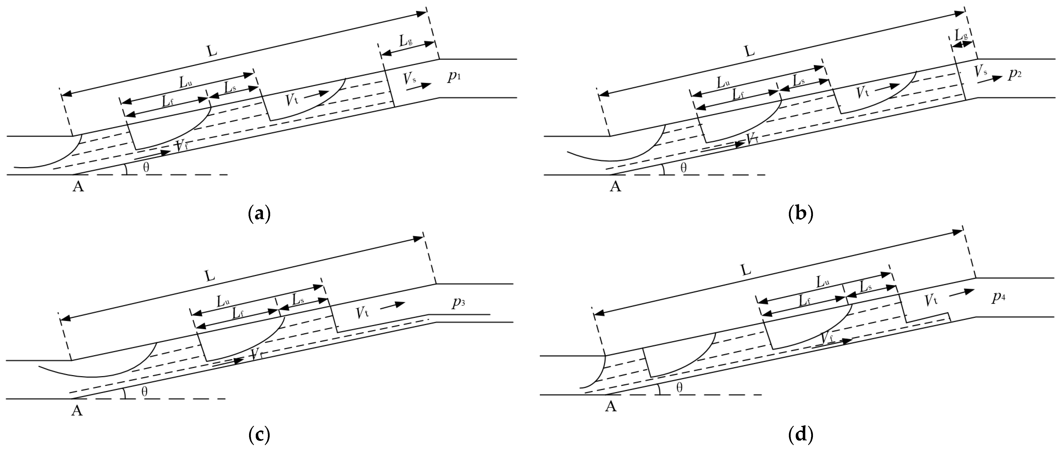
3.2. Slug Flow Pressure Model in Inclined Pipe
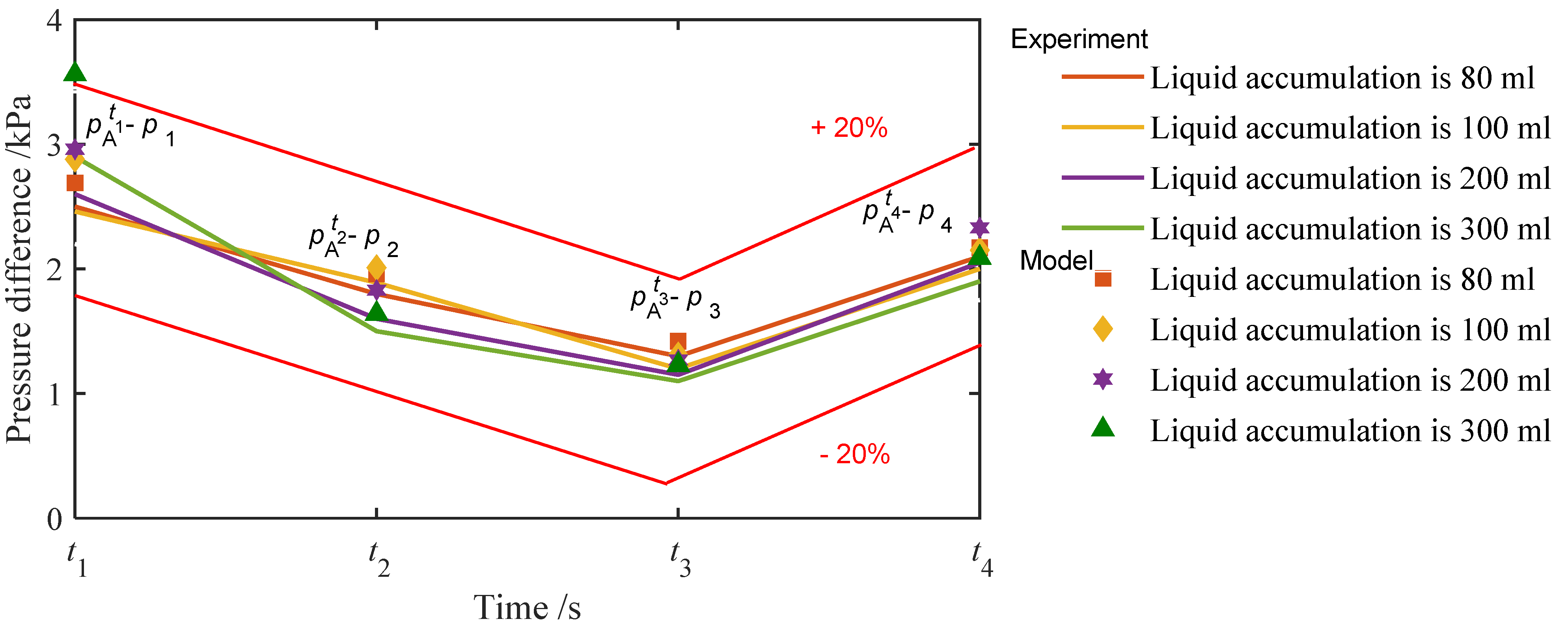
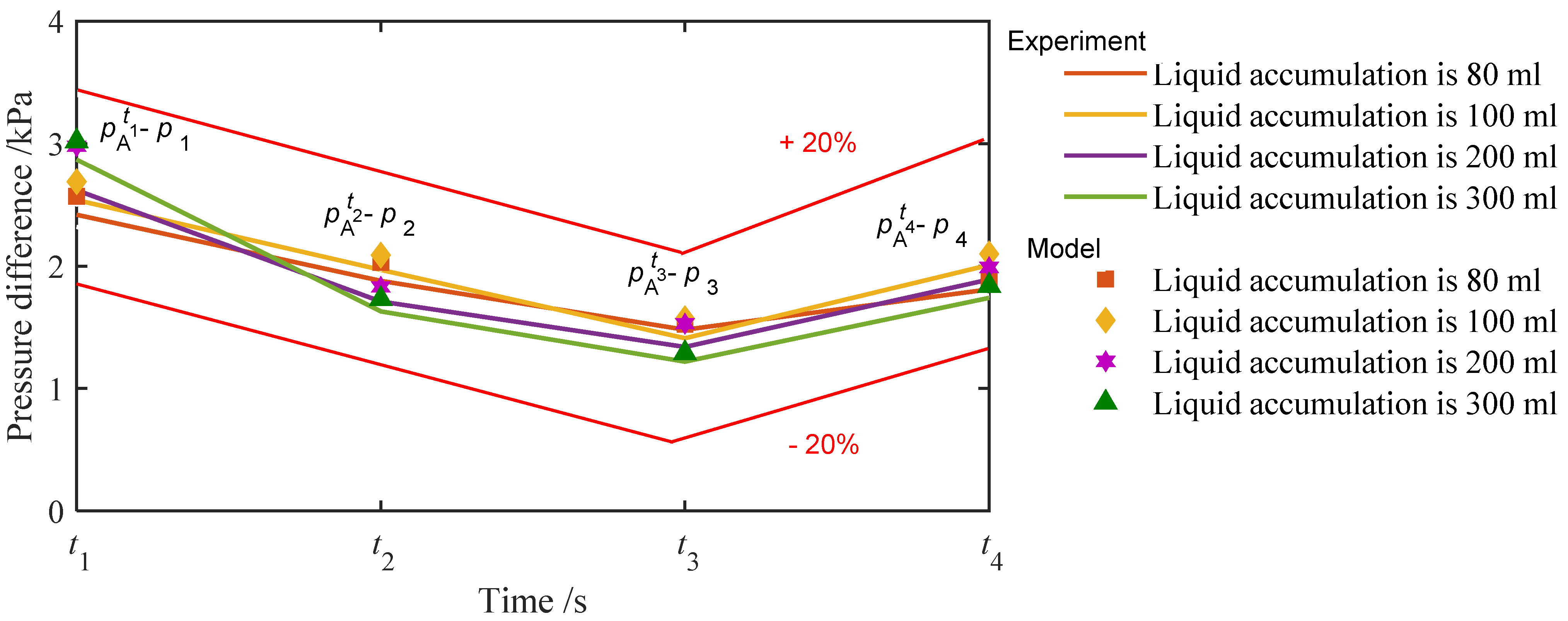
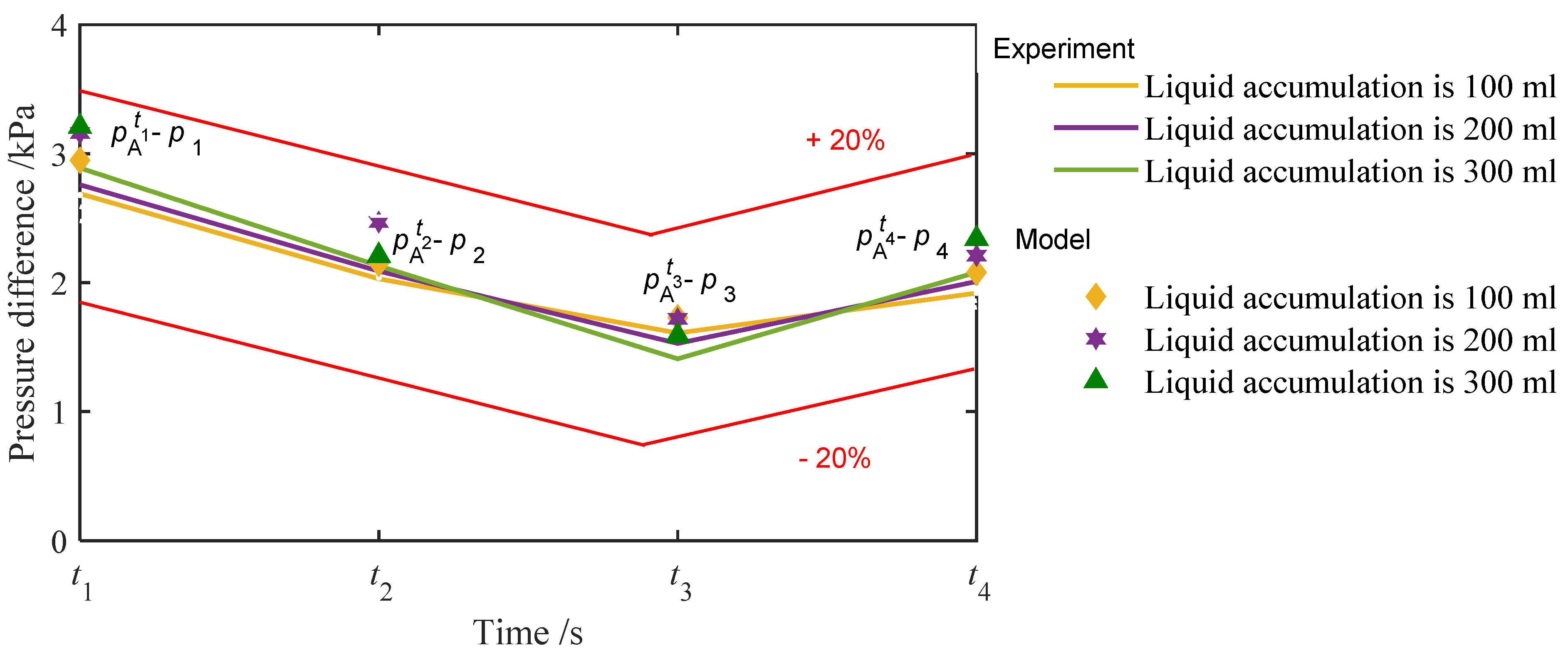
4. Results and Discussion
5. Conclusions
Author Contributions
Funding
Institutional Review Board Statement
Informed Consent Statement
Data Availability Statement
Conflicts of Interest
References
- Evans, D.; Parkes, D.; Dooner, M.; Williamson, P.; Williams, J.; Busby, J.; He, W.; Wang, J.; Garvey, S. Salt cavern exergy storage capacity potential of UK massively bedded halites, using compressed air Energy storage (CAES). Appl. Sci. 2021, 11, 4728. [Google Scholar] [CrossRef]
- Huang, S.; Khajepour, A. A new adiabatic compressed air energy storage system based on a novel compression strategy. Energy 2022, 242, 122883. [Google Scholar] [CrossRef]
- Han, Z.; Ma, F.; Wu, D.; Zhang, H.; Dong, F.; Li, P.; Xiao, L. Collaborative optimization method and operation performances for a novel integrated energy system containing adiabatic compressed air energy storage and organic Rankine cycle. J. Energy Storage 2021, 41, 102942. [Google Scholar] [CrossRef]
- Shaqsi, A.Z.A.; Sopian, K.; Al-Hinai, A. Review of energy storage services, applications, limitations, and benefits. Energy Rep. 2020, 6, 288–306. [Google Scholar] [CrossRef]
- Yu, Q.; Li, X.; Geng, Y.; Tan, X. Study on quasi-isothermal expansion process of compressed air based on spray heat transfer. Energy Rep. 2022, 8, 1995–2007. [Google Scholar] [CrossRef]
- Heidari, M.; Parra, D.; Patel, M.K. Physical design, techno-economic analysis and optimization of distributed compressed air energy storage for renewable energy integration. J. Energy Storage 2021, 35, 102268. [Google Scholar] [CrossRef]
- Mousavi, S.B.; Nabat, M.H.; Razmi, A.R.; Ahmadi, P. A comprehensive study and multi-criteria optimization of a novel sub-critical liquid air energy storage (SC-LAES). Energy Convers. Manag. 2022, 258, 115549. [Google Scholar] [CrossRef]
- Li, H.; Li, W.; Zhang, X.; Zhu, Y.; Zuo, Z.; Chen, H.; Yu, Z. Performance and flow characteristics of the liquid turbine for supercritical compressed air energy storage system. Appl. Therm. Eng. 2022, 211, 118491. [Google Scholar] [CrossRef]
- Wang, Z.; Wang, J.; Cen, H.; Ting, D.S.; Carriveau, R.; Xiong, W. Large-eddy simulation of a full-scale underwater energy storage accumulator. Ocean Eng. 2021, 234, 109184. [Google Scholar] [CrossRef]
- Wang, H.; Wang, Z.; Liang, C.; Carriveau, R.; Ting, D.S.-K.; Li, P.; Cen, H.; Xiong, W. Underwater Compressed Gas Energy Storage (UWCGES): Current Status, Challenges, and Future Perspectives. Appl. Sci. 2022, 12, 9361. [Google Scholar] [CrossRef]
- Liang, C.; Xiong, W.; Wang, Z. Flow characteristics simulation of concave pipe with zero net liquid flow. Energy Rep. 2022, 8, 775–782. [Google Scholar] [CrossRef]
- Xu, Z.; Yang, H.; Xie, Y.; Zhu, J.; Liu, C. Thermodynamic analysis of a novel adiabatic compressed air energy storage system with water cycle. J. Mech. Sci. Technol. 2022, 36, 3153–3164. [Google Scholar] [CrossRef]
- Guo, C.; Li, C.; Zhang, K.; Cai, Z.; Ma, T.; Maggi, F.; Gan, Y.; El-Zein, A.; Pan, Z.; Shen, L. The promise and challenges of utility-scale compressed air energy storage in aquifers. Appl. Energy 2021, 286, 116513. [Google Scholar] [CrossRef]
- Liang, C.; Xiong, W.; Carriveau, R.; Ting, D.S.; Wang, Z. Experimental and modeling investigation of critical slugging behavior in marine compressed gas energy storage systems. J. Energy Storage 2022, 49, 104038. [Google Scholar] [CrossRef]
- Calado, G.; Castro, R. Hydrogen production from offshore wind parks: Current situation and future perspectives. Appl. Sci. 2021, 11, 5561. [Google Scholar] [CrossRef]
- Wang, H.; Tong, Z.; Dong, X.; Xiong, W.; Ting, D.S.-K.; Carriveau, R.; Wang, Z. Design and energy saving analysis of a novel isobaric compressed air storage device in pneumatic systems. J. Energy Storage 2021, 38, 102614. [Google Scholar] [CrossRef]
- Guo, H.; Xu, Y.; Zhu, Y.; Zhang, X.; Yin, Z.; Chen, H. Coupling properties of thermodynamics and economics of underwater compressed air energy storage systems with flexible heat exchanger model. J. Energy Storage 2021, 43, 103198. [Google Scholar] [CrossRef]
- Crespi, E.; Mammoliti, L.; Colbertaldo, P.; Silva, P.; Guandalini, G. Sizing and operation of energy storage by Power-to-Gas and Underwater Compressed Air systems applied to offshore wind power generation. In Proceedings of the 76th Congresso Nazionale ATI (ATI 2021), Rome, Italy, 15–17 September 2021; pp. 1–18. [Google Scholar]
- Astolfi, M.; Guandalini, G.; Belloli, M.; Hirn, A.; Silva, P.; Campanari, S. Preliminary design and performance assessment of an underwater compressed air energy storage system for wind power balancing. J. Eng. Gas Turbines Power 2020, 142, 091001. [Google Scholar] [CrossRef]
- Zhang, X.; Qin, C.C.; Loth, E.; Xu, Y.; Zhou, X.; Chen, H. Arbitrage analysis for different energy storage technologies and strategies. Energy Rep. 2021, 7, 8198–8206. [Google Scholar] [CrossRef]
- Chen, W.; Xu, H.-L.; Kong, W.-Y.; Yang, F.-Q. Study on three-phase flow characteristics of natural gas hydrate pipeline transmission. Ocean Eng. 2020, 214, 107727. [Google Scholar] [CrossRef]
- Rastogi, A.; Fan, Y. Experimental and modeling study of onset of liquid accumulation. J. Nat. Gas Sci. Eng. 2020, 73, 103064. [Google Scholar] [CrossRef]
- Chen, S.; Zhang, Y.; Wang, X.; Teng, K.; Gong, Y.; Qu, Y. Numerical simulation and experiment of the gas-liquid two-phase flow in the pigging process based on bypass state. Ocean Eng. 2022, 252, 111184. [Google Scholar] [CrossRef]
- Gonçalves, J.L.; Mazza, R.A. A transient analysis of slug flow in a horizontal pipe using slug tracking model: Void and pressure wave. IJMF 2022, 149, 103972. [Google Scholar] [CrossRef]
- An, H.-J.; Langlinais, J.P.; Scott, S. Effects of density and viscosity in vertical zero net liquid flow. J. Energy Resour. Technol. 2000, 122, 49–55. [Google Scholar] [CrossRef]
- Amaravadi, S. The effect of pressure on two-phase zero-net liquid flow in inclined pipes. In Proceedings of the SPE Annual Technical Conference and Exhibition, New Orleans, LA, USA, 25–28 September 1994. [Google Scholar]
- Gregory, G.; Aziz, K.; Nicholson, M. Gas-liquid flow in upwards inclined pipe with zero net liquid production. In Proceedings of the PSIG Annual Meeting, Colorado Springs, CO, USA, 22–23 October 1981. [Google Scholar]
- Kokal, S.; Stanislav, J. An analysis of two-phase flow in inclined pipes with zero net liquid production. J. Can. Pet. Technol. 1986, 25, PETSOC-86-06-08. [Google Scholar] [CrossRef] [PubMed]
- Amaravadi, S.; Minami, K.; Shoham, O. Two-phase zero-net liquid flow in upward inclined pipes: Experiment and modeling. SPE J. 1998, 3, 253–260. [Google Scholar] [CrossRef]
- Zhu, H.; Gao, Y.; Zhao, H. Experimental investigation on the flow-induced vibration of a free-hanging flexible riser by internal unstable hydrodynamic slug flow. Ocean Eng. 2018, 164, 488–507. [Google Scholar] [CrossRef]
- Dukler, A.E.; Hubbard, M.G. A model for gas-liquid slug flow in horizontal and near horizontal tubes. Ind. Eng. Chem. Fundam. 1975, 14, 337–347. [Google Scholar] [CrossRef]
- Gregory, G.; Scott, D. Correlation of liquid slug velocity and frequency in horizontal cocurrent gas-liquid slug flow. AIChE J. 1969, 15, 933–935. [Google Scholar] [CrossRef]
- Wallis, G.B. Critical two-phase flow. IJMF 1980, 6, 97–112. [Google Scholar] [CrossRef]
- Fabre, J. Advancements in two-phase slug flow modeling. In Proceedings of the University of Tulsa Centennial Petroleum Engineering Symposium, Tulsa, OK, USA, 29–31 August 1994. [Google Scholar]
- Felizola, H.; Shoham, O. A unified model for slug flow in upward inclined pipes. J. Energy Resour. Technol. 1995, 117, 7–12. [Google Scholar] [CrossRef]
- Bendiksen, K.H.; Malnes, D.; NYDAL, O.J. On the modelling of slug flow. Chem. Eng. Commun. 1996, 141, 71–102. [Google Scholar] [CrossRef]
- Colmenares, J.; Ortega, P.; Padrino, J.; Trallero, J. Slug flow model for the prediction of pressure drop for high viscosity oils in a horizontal pipeline. In Proceedings of the SPE International Thermal Operations and Heavy Oil Symposium, Porlamar, Venezuela, 12–14 March 2001. [Google Scholar]
- Zhang, H.-Q.; Wang, Q.; Sarica, C.; Brill, J.P. Unified model for gas-liquid pipe flow via slug dynamics—Part 1: Model development. J. Energy Resour. Technol. 2003, 125, 266–273. [Google Scholar] [CrossRef]
- Dong, C.; Qi, R.; Zhang, L. Flow and heat transfer for a two-phase slug flow in horizontal pipes: A mechanistic model. Phys. Fluids 2021, 33, 034117. [Google Scholar] [CrossRef]
- Dong, C.; Qi, R.; Zhang, L. Mechanistic modeling of flow and heat transfer in vertical upward two-phase slug flows. Phys. Fluids 2022, 34, 013309. [Google Scholar] [CrossRef]
- Zhu, H.; Gao, Y.; Zhao, H. Experimental investigation of slug flow-induced vibration of a flexible riser. Ocean Eng. 2019, 189, 106370. [Google Scholar] [CrossRef]
- Kim, H.-G.; Kim, S.-M. Experimental investigation of flow and pressure drop characteristics of air-oil slug flow in a horizontal tube. Int. J. Heat Mass Transf. 2022, 183, 122063. [Google Scholar] [CrossRef]
- Liu, A.; Cheng, L.; Yan, C. Experimental study on length, liquid film thickness and pressure drop of slug flow in horizontal narrow rectangular channel. Chem. Eng. Res. Des. Trans. Inst. Chem. Eng. 2022, 182, 502–516. [Google Scholar] [CrossRef]
- Al-Dogail, A.S.; Gajbhiye, R.N. Effects of Density, Viscosity and Surface Tension on Flow Regimes and Pressure Drop of Two-Phase Flow in Horizontal Pipes. J. Pet. Sci. Eng. 2021, 205, 108719. [Google Scholar] [CrossRef]
- Zhao, Y.; Lao, L.; Yeung, H. Investigation and prediction of slug flow characteristics in highly viscous liquid and gas flows in horizontal pipes. Chem. Eng. Res. Des. 2015, 102, 124–137. [Google Scholar] [CrossRef]
- Scott, S.; Kouba, G. Advances in slug flow characterization for horizontal and slightly inclined pipelines. In Proceedings of the SPE Annual Technical Conference and Exhibition, New Orleans, LA, USA, 23–26 September 1990. [Google Scholar]
- Wang, Y.; Yan, C.; Sun, L.; Yan, C.; Tian, Q. Characteristics of slug flow in a narrow rectangular channel under inclined conditions. Prog. Nucl. Energy 2014, 76, 24–35. [Google Scholar] [CrossRef]
- Andreussi, P.; Minervini, A.; Paglianti, A. Mechanistic model of slug flow in near-horizontal pipes. AIChE J. 1993, 39, 1281–1291. [Google Scholar] [CrossRef]
- Crawford, T.J.; Weinberger, C.B.; Weisman, J. Two-phase flow patterns and void fractions in downward flow. Part II: Void fractions and transient flow patterns. Int. J. Multiph. Flow 1986, 12, 219–236. [Google Scholar] [CrossRef]


| Water | Air | |
|---|---|---|
| Density | 997.05 kg∙m−3 | 1.184 kg∙m−3 |
| Kinetic Viscosity | 8.9008 × 10⁻⁴ Pa∙s | 1.849 × 10⁻⁵ Pa∙s |
| Surface Tension | σA/W = 0.07197 N∙m−1 | |
| Parameter | Expression |
|---|---|
| Gas phase wetting perimeter SG | |
| Liquid phase wetting perimeter SL | |
| Cross sectional area of pipe A | |
| Gas phase cross-sectional area AG | |
| Liquid phase cross-sectional area AL | |
| Shear force of liquid film and wall τf | |
| Shear force of gas phase and wall τG | |
| Shear stress in the liquid slug area τs | |
| Friction coefficient of liquid film and wall fL | |
| Friction coefficient of gas phase and wall fG | |
| Friction factor between gas and phase in liquid slug area fs | |
| Hydraulic diameter of liquid phase DL |
Disclaimer/Publisher’s Note: The statements, opinions and data contained in all publications are solely those of the individual author(s) and contributor(s) and not of MDPI and/or the editor(s). MDPI and/or the editor(s) disclaim responsibility for any injury to people or property resulting from any ideas, methods, instructions or products referred to in the content. |
© 2023 by the authors. Licensee MDPI, Basel, Switzerland. This article is an open access article distributed under the terms and conditions of the Creative Commons Attribution (CC BY) license (https://creativecommons.org/licenses/by/4.0/).
Share and Cite
Liang, C.; Xiong, W.; Wang, M.; Ting, D.S.K.; Carriveau, R.; Wang, Z. Experimental and Modeling Investigation for Slugging Pressure under Zero Net Liquid Flow in Underwater Compressed Gas Energy Storage Systems. Appl. Sci. 2023, 13, 1216. https://doi.org/10.3390/app13021216
Liang C, Xiong W, Wang M, Ting DSK, Carriveau R, Wang Z. Experimental and Modeling Investigation for Slugging Pressure under Zero Net Liquid Flow in Underwater Compressed Gas Energy Storage Systems. Applied Sciences. 2023; 13(2):1216. https://doi.org/10.3390/app13021216
Chicago/Turabian StyleLiang, Chengyu, Wei Xiong, Meiling Wang, David S. K. Ting, Rupp Carriveau, and Zhiwen Wang. 2023. "Experimental and Modeling Investigation for Slugging Pressure under Zero Net Liquid Flow in Underwater Compressed Gas Energy Storage Systems" Applied Sciences 13, no. 2: 1216. https://doi.org/10.3390/app13021216
APA StyleLiang, C., Xiong, W., Wang, M., Ting, D. S. K., Carriveau, R., & Wang, Z. (2023). Experimental and Modeling Investigation for Slugging Pressure under Zero Net Liquid Flow in Underwater Compressed Gas Energy Storage Systems. Applied Sciences, 13(2), 1216. https://doi.org/10.3390/app13021216