AE-DTI: An Efficient Darknet Traffic Identification Method Based on Autoencoder Improvement

Abstract

With the continuous expansion of the darknet and the increase in various criminal activities in the darknet, darknet traffic identification has become increasingly essential. However, existing darknet traffic identification methods rely on all traffic characteristics, which require a long computing time and a large amount of system resources, resulting in low identification efficiency. To this end, this paper proposes an autoencoder-based darknet traffic identification method (AE-DTI). First, AE-DTI maps the feature values to pixels of a two-dimensional grayscale image after deduplication and denoising of the darknet traffic dataset. Then, AE-DTI designs a new feature selection algorithm (AE-FS) to downscale the grayscale graph, and AE-FS trains a feature scoring network, which globally scores all the features based on the reconstruction error to select the features with scores greater than or equal to a set threshold value. Finally, AE-DTI uses a one-dimensional convolutional neural network with a dropout layer to identify darknet traffic on the basis of alleviating overfitting. Experimental results on the ISCXTor2016 dataset show that, compared with other dimensionality reduction methods (PCA, LLE, ISOMAP, and autoencoder), the classification model trained with the data obtained from AE-FS has a significant improvement in classification accuracy and classification efficiency. Moreover, AE-DTI also shows significant improvement in recognition accuracy compared with other models. Experimental results on the CSE-CIC-IDS2018 dataset and CIC-Darknet2020 dataset show that AE-DTI has strong generalization.

1. Introduction

The darknet refers to certain cyberspaces not included by ordinary search engines [1], also known as the deep web. On the darknet, users can anonymously access and share various information and content, including illegal and dangerous content such as drugs, weapons, terrorist propaganda, and more. Therefore, the darknet has also become the focus of governments and law enforcement agencies of various countries, and the traffic identification of the darknet has become an essential means of monitoring and combating crimes on the darknet [2].

Traffic identification refers to identifying specific network traffic types by analyzing and processing network data packets [3]. There are two main existing traffic identification methods [4]. The machine learning-based method: this method builds a traffic identification model by training with known normal traffic and dark network traffic; the model can learn the characteristics and patterns of different types of traffic and is used to identify unknown traffic. The deep learning-based method: This method employs deep neural networks to learn high-level features in network traffic. Deep learning methods can automatically learn and represent complex features, so it is very suitable for processing large-scale network traffic data.

However, the existing darknet traffic identification relies on all traffic characteristics, which requires a long computing time and a large amount of system resources, resulting in low identification efficiency. To this end, this paper proposes an autoencoder-based darknet traffic identification method (AE-DTI). First, AE-DTI maps the feature values to pixels of a two-dimensional grayscale image after deduplication and denoising of the darknet traffic dataset. Then, AE-DTI designs a new feature selection algorithm (AE-FS) to downscale the grayscale graph, and AE-FS trains a feature scoring network, which globally scores all the features based on the reconstruction error to select the features with scores greater than or equal to a set threshold value. Finally, AE-DTI uses a one-dimensional convolutional neural network with a dropout layer to identify darknet traffic on the basis of alleviating overfitting.

2. Related Research

2.1. Machine Learning Methods

Wei Li et al. [5] proposed a machine learning method using a C4.5 decision tree, which accurately classifies real-time traffic by collecting 12 features without inspecting the payload of packets. Experimental results show that the method has high accuracy in traffic classification. Dong et al. [6] conducted research on the identification and classification of Skype traffic. They introduced a Netflow Flow Identification (NFI) mechanism based on Naive Bayes to address the challenges of real-time tracking and limited labeled data. Xu et al. [7] proposed a feature engineering approach utilizing sliding windows to transform Tor traffic into 12 different types of features. They employed machine learning models, including XGBoost and random forest, as downstream classifiers, achieving promising accuracy results. Xin Tong et al. [8] introduced a traffic analysis method known as “Dark-Forest”. This approach uses the particle swarm optimization algorithm to select relevant features from dark network traffic. The selected features are then classified using the DeepForest model for further analysis. Liu, Z et al. [9] proposed ELD (Extending Labeled Data) to identify new unknown mobile traffic labels to extend labeled mobile traffic data. The ELD method employs a hierarchical approach to traffic identification, which involves analyzing data packet headers, data packet payloads, and traffic statistics. Various techniques, such as ServerTag, payload distribution inspection, and random forest, are used to accomplish the traffic identification tasks at each level. Chen, Y et al. [10] proposed a new method called Federated Deep Autoencoded Gaussian Mixture Model (FDAGMM) to improve performance problems caused by insufficient data in unsupervised anomaly detection tasks through federated learning. FDAGMM comprehensively uses dimensionality reduction and density estimation techniques to optimize model performance and protect data privacy. The experiment proves the superiority of FDAGMM in dealing with limited data and brings a new solution to the field of network security.

2.2. Deep Learning Methods

Karagiannis et al. [11] conducted a study on the multi-level behavioral characteristics of traffic, including inter-host interactions, protocol usage, and average packet size. They employed convolutional neural networks to effectively identify and classify these distinctive features. Wei Wang et al. [12] introduced a traffic classification approach that leverages a text convolutional neural network. This method represents traffic data as vectors and uses the text convolutional neural network to extract crucial features for classification. Tong et al. [13] proposed a real-time classification method that selected the eight most effective stream-level features and combined them into six feature sets. Wang et al. [14] proposed a two-stage model that utilizes spatio-temporal features to identify malicious attacks on the network. First, each packet is thermally encoded and fed into a CNN to obtain spatial features, and then an RNN is used to learn the overall temporal features. E. Hodo et al. [15] used an artificial neural network and a support vector machine for binary classification of the public dataset ISCXTor2016 and achieved satisfactory accuracies. Huo, Y et al. [16]. proposed a new classification model. The model extracts spatial features through the CNN layer, obtains temporal features through the LSTM layer, and then fuses multi-scale features and improves feature representation capabilities through the attention mechanism. Experiments on the ISCXTor2016 dataset have lower loss and higher accuracy. Ying Zhao et al. [17] proposed a method called MT-DNN-FL (Application of Multi-task Deep Neural Network in Federated Learning). Through federated learning, multiple participants can jointly train the global model without sharing the training data with the server, thereby preventing the training data from being used by attackers. Experimental results show that the proposed method achieves better detection and classification performance on datasets such as ISCXTor2016 compared to baseline methods based on centralized training architectures. F. Meslet-Millet et al. [18] proposed a novel deep learning architecture called SPPNet for real-time network traffic classification. Through a deep understanding of the features used by deep learning models in classification, improved data processing overcomes the threat to traditional classification tools due to the widespread encryption of communications. This method can analyze the information carried in the header of the data packet and realize the accurate classification of the dark network traffic, which effectively improves the performance of the classification process. He et al. [19] proposed a method for analyzing anonymous proxy traffic by converting the size sequence and inter-arrival time sequence of the initial N data packets of the flow into images. These images were then classified using a one-dimensional convolutional neural network. The approach demonstrated excellent performance in the detection of Shadowsocks traffic and VPN traffic, achieving a significant reduction in image size while maintaining satisfactory results. Salman, O et al. [20] proposed an unsupervised deep learning model for detecting mutated network traffic, implemented through a generative deep learning architecture (including autoencoders and generative adversarial networks). Experimental results show that the model has achieved remarkable results in denoising and detecting forged traffic, which provides an effective method for improving network security.

2.3. Method Summary

Based on our investigation into the aforementioned approaches, it has been determined that both machine learning and deep learning have demonstrated impressive outcomes in the realm of traffic identification. Nevertheless, deep learning exhibits exceptional performance and holds vast potential for application, particularly in the identification of dark web traffic. However, it should be noted that due to the intricacy of neural networks, achieving optimal recognition results necessitates substantial computational resources. Consequently, in the field of flow recognition, striking a balance between high efficiency and accuracy has become a central concern. Consequently, Section 3 will expound upon our proposed method (AE-DTI), which offers a novel solution to this predicament by simultaneously upholding recognition efficiency and accuracy.

3. AE-DTI Model Design

This section mainly introduces the model design of the autoencoder-based darknet traffic identification method (AE-DTI). AE-DTI mainly consists of two parts: feature selection and traffic identification. In the feature selection part, AE-DTI designed a new feature selection algorithm (AE-FS) to perform feature selection on the grayscale image and then reshape the selected features into one-dimensional data. In the traffic identification part, the reshaped one-dimensional data is used to train a one-dimensional convolutional neural network with a dropout layer to identify darknet traffic. The AE-DTI flow chart is shown in Figure 1.

3.1. AE-FS Feature Selection Algorithm Design

This section details the design principle and implementation process of the AE-FS algorithm.

3.1.1. AE-FS Algorithm Principle

Data dimensionality reduction is a crucial task in reducing the dimensions of data while preserving essential information. Autoencoder, a powerful method for dimensionality reduction, utilizes neural networks to learn the mapping relationship between the high-dimensional representation of data and its compressed representation. In comparison to linear methods, autoencoder excels in capturing the nonlinear structure of complex data. Furthermore, it is capable of adaptively learning the optimal feature representation without the need for a predefined feature extraction method. The conventional autoencoder operates as an unsupervised algorithm. Initially, it compresses the input image, denoted as $A,$ through a neural network to extract critical features from the data. Subsequently, it reconstructs the data as $A^{\prime }$ by decoding these important features. By comparing the errors between $A$ and the reconstructed data $A^{\prime },$ the reverse gradient is updated iteratively to enhance the accuracy of the autoencoder. Following model training, the first half of the network can be selected to compress the dataset effectively, achieving the objective of dimensionality reduction. The specific network structure is illustrated in Figure 2. Building upon the traditional autoencoder dimensionality reduction method, AU-FS has been devised as outlined below.

First, AE-FS uses the original dataset to train the autoencoder and calculates the reconstruction error l. Then, the AE-FS systematically eliminates each feature individually and re-trains the autoencoder model to obtain a new reconstruction error $l^{\prime }$. Finally, AE-FS calculates the score of each removed feature by comparing the difference value between l and $l^{\prime },$ thereby selecting those features whose scores are higher than a set threshold. In short, AE-FS mainly evaluates the importance of each feature globally by training a feature scoring network and then selects key features to reshape one-dimensional data according to the set scoring threshold. The network structure diagram is shown in Figure 3.

3.1.2. AE-FS Algorithm Implementation Process

Implementing the AE-FS algorithm includes two modules: feature global scoring and key feature extraction. To facilitate the explanation of the implementation process of AE-FS, suppose there is a two-dimensional grayscale dataset $Q=\left\{X_1,X_2,\dots ,X_i,\dots ,X_k\right\},i\in \left[1,k\right],$ where k represents the sample of the dataset quantity, $X_i$ represents the two-dimensional grayscale image in the dataset., and each $X_i$ has m pixels (that is, m features).

Feature Global Scoring

The feature global score mainly includes three steps: initial reconstruction error calculation, ablation error calculation, and feature score calculation, which are described in detail as follows.

Step 1: Initial reconstruction error calculation.

The $X_i=\{x_1,x_2,{\dots ,x}_j,\dots ,x_m\},$ $j\in \left[1,m\right]$ in the dataset $Q$ is sequentially input into the autoencoder for training, and the decoder outputs $X_i$’${=\{x}_1^{\prime },x_2^{\prime },{\dots ,x}_j^{\prime },\dots ,x_m^{\prime }\},j\in \left[1,m\right]$. Use the mean square error to calculate the reconstruction error of each $X_i$ and $X_i^{\prime }$ in turn, accumulate and take the average to obtain the reconstruction error $L\left(Q\right)$ of the dataset $Q,$ referred to as $L$, as shown in Formula (1).

$$L(Q)=\frac{1}{k}\sum _{i=1}^k\frac{1}{m}\sum _{j=1}^m{(x_j-x_j^{\prime })}^2$$

(1)

Step 2: Ablation error calculation.

The m features in the dataset $Q$ are sequentially removed to obtain a new dataset $Q_j=\{X_1^j,X_2^j,{\dots ,X}_i^j,\dots ,X_k^j\}$ $,i\in \left[1,k\right]$, $j\in \left[1,m\right]$. $Q_j$ means removal from the dataset of the jth feature, $X_i^j$ represents the grayscale image of the jth feature removed from the dataset. Input $X_i^j$ in $Q_j$ to the autoencoder in turn for training, and the decoder outputs $X_i^{j\prime }$. Additionally, use Formula (1) to calculate the reconstruction error of each $X_i^j$ and $X_i^{j\prime }$ to obtain the reconstruction error $L\left(Q_j\right)$ of the dataset $Q_j$, referred to as $L_j$.

Step 3: Feature score calculation.

The significance of each feature is assessed by comparing the discrepancy ${\tau }_j$ between the error values $L$ and $L_j$. A larger value of the difference degree ${\tau }_j$ means that the feature is more essential, and the corresponding score is higher. To exclude the influence of negative values on the results, AE-FS uses the relative error to calculate the difference degree ${\tau }_j,$ which is calculated as in Formula (2).

$${\tau }_j=\frac{|L-L_j|}{\left|L\right|}$$

(2)

To briefly illustrate the process of AE-FS’s feature global scoring, a 3 ∗ 3 (a total of 9 features) image dataset is used as an example to illustrate. First, the 3 ∗ 3 image dataset is passed into the autoencoder for training, and the reconstruction error value calculated by AE-FS is 0.01. Then, AE-FS removes the 1st, 2nd, 3rd, 4th, …, 9th features, respectively, to obtain 9 different datasets. Next, AE-FS inputs the 9 datasets into the self-encoder for training in sequence, and calculates the corresponding reconstruction error values: 0.04, 0.02, 0.03, 0.01, 0.05, 0.005, 0.012, 0.003, and 0.025. Finally, AE-FS calculates the difference degree (score) of the two reconstruction errors through the relative error (Formula (2)), and the obtained scores are: 3, 1, 2, 0, 4, 0.5, 0.2, 0.7, and 1.5. The specific data are shown in

Table 1. Feature global scoring results.

FEA	OREV	ROREV	FSV
x1	0.01	0.04	3
x2	0.01	0.02	1
x3	0.01	0.03	2
x4	0.01	0.01	0
x5	0.01	0.05	4
x6	0.01	0.005	0.5
x7	0.01	0.012	0.2
x8	0.01	0.003	0.7
x9	0.01	0.025	1.5

.

In Table 1, FEA represents the feature, OREV represents the reconstruction error value of the original dataset, ROREV represents the reconstruction error value of the dataset after deleting a certain feature, and FSV represents the feature difference degree (score). A higher FSV value indicates a more crucial feature.

Key Feature Extraction

The extraction of key features mainly includes two steps: key feature screening and positioning, and key feature matching and reshaping, which are described in detail as follows.

Step 1: Key feature screening and positioning.

After AE-FS calculates a score for each feature in $X_i$, AE-FS establishes a Cartesian coordinate system for $X_i,$ where both X and Y axes take positive values. AE-FS traverses and addresses the X-axis and Y-axis at the same time, looks for features with a score greater than or equal to the threshold σ, and records its position in the Cartesian coordinate system, as shown in Formula (3).

$$set\left\{\left(x,y\right)\right\}=\left\{{Loop\left(x\right)}_{y=0}^{\sqrt{m}}\&{Loop\left(y\right)}_{x=0}^{\sqrt{m}}\right\}\&\left[{\tau }_j\left(x,y\right)\ge \mathsf{\sigma }\right]$$

(3)

${Loop\left(x\right)}_{x=0}^{\sqrt{m}}$ means X-axis loop accumulation traversal, ${Loop\left(y\right)}_{y=0}^{\sqrt{m}}$ means Y-axis loop accumulation traversal, ${\tau }_j\left(x,y\right)$ means the coordinate points of the score feature j, and $set\left\{\left(x,y\right)\right\}$ means the set of key feature coordinates.

Step 2: Key feature matching and reshaping.

According to the coordinate parameters in $set\left\{\left(x,y\right)\right\},$ AE-FS addresses the Y-axis and X-axis at the same time, and quickly screens the features of the original dataset $Q,$ so as to realize the feature selection of the dataset, as shown in Formula (4).

$$Subset (Q_n)=\mathrm{Map}(Q\ast set\left\{\left(x,y\right)\right\}\&\left\{{Loop\left(x\right)}_{y=0}^{\sqrt{m}}\&{Loop\left(y\right)}_{x=0}^{\sqrt{m}}\right\}$$

(4)

$Subset$ ($Q_n$) represents the subset of dataset $Q$ after n (n < m) features are selected by AE-FS. AE-FS reshapes the one-dimensional data sequentially according to the sample order of dataset $Q$ and obtains the number of features n in the one-dimensional dataset.

For example, when AE-FS scores each feature of the 3 ∗ 3 (9 features in total) picture dataset (as shown in Table 1), first, AE-FS sets the threshold ($\mathsf{\sigma }$) to 1. Then, it filters out the features with a score greater than or equal to the threshold ($\mathsf{\sigma }$), and saves the corresponding coordinates (0, 1), (0, 2), (1, 2), and (2, 1). Then, it quickly performs feature matching on the 3 ∗ 3 (a total of 9 features) image dataset through the saved coordinate points. Finally, AE-FS reshapes the filtered features into one-dimensional data. The process Is shown in Figure 4.

AE-FS Algorithm Process Description

In summary, the AE-FS algorithm process can be outlined based on the description of the two key modules: AE-FS feature global scoring and key feature extraction. The detailed algorithm process is presented in Algorithm 1.

Algorithm 1: AE-FS algorithm process

Input:$\mathrm{Sample} \mathrm{set} Q=\left\{X_1,X_2,\dots ,X_i,\dots ,X_k\right\},$$\mathrm{where} i\in \left[1,k\right]$. The number of features per sample is m.

Process: For i = 1, 2, 3,…, k do:    Autoencoder $=\mathrm{Decoder} (\mathrm{Encoder} (X_i$)) # Self-encoder model training; $X_i$$\prime = \mathrm{Autoencoder} (X_i$); $L=Reconstruction errors$$(X_i$’$,X_i$) # Calculate the reconfiguration error of the autoencoder L; For j = 1, 2, 3,…, m do:    $X_i^{j\prime }$$=\mathrm{Autoencoder} \left(X_i^j\right)$;     $L_j=Reconstruction errors$ ($X_i^j,$ $X_i^{j\prime }$) # After deleting a feature, calculate the new reconstruction error;    ${\tau }_j$$=\mathrm{Relative} \mathrm{Error} (L,L_j$) # Calculate the score of each feature by relative error;    $\mathrm{Value} \left[j\right]=\{{\tau }_j$, (x, y)} # Store each feature value and the corresponding coordinates in a set; Select (Value [j] ≥ σ) # Filter all features with feature scores greater than σ; Reshape (Value [j]) # Reshaping one-dimensional data.

3.2. CNN-Based Dark Network Traffic Recognition Model Design

A convolutional neural network (CNN) consists of key components such as the convolutional layer, activation function, pooling layer, fully connected layer, and loss function. Utilizing large-scale training data and back-propagation algorithms, CNN has the ability to automatically adjust network parameters, enabling it to learn optimal feature representations and adapt to diverse tasks and data. Building upon this concept, this paper designs a one-dimensional convolutional model, known as traffic identification-CNN (TI-CNN), specifically designed for traffic classification. The TI-CNN network structure is designed as follows: in the convolutional pooling computation stage, TI-CNN is designed with three layers of convolution and three layers of pooling; in the classification stage, TI-CNN adds a dropout layer after two fully connected layers. The network structure is shown in Figure 5.

The TI-CNN convolution process is shown in Formula (5) where f denotes the original one-dimensional image, g denotes the convolution kernel, and o denotes the position in the output result. $\cdot$ denotes the dot product operation, where two numbers are multiplied. z is the offset inside the convolution kernel, and the convolution kernel g is slid over the original image f. For each position o, the output result $f\ast g\left[o\right]$ is obtained by dot multiplying and summing the convolution kernel g with the corresponding position of f at o.

$$(f\ast g)[o]=\sum _{\mathrm{k}=-\mathrm{\infty }}^{\mathrm{\infty }}f\left[z\right]·g[o-z]$$

(5)

To reduce feature size and computational complexity, TI-CNN employs average pooling. Additionally, to address the issue of vanishing gradients associated with the Sigmod() and Tanh() functions, TI-CNN adopts the ReLU() function as the activation function, as in Formula (6). When the input x is greater than or equal to 0, the output of the ReLU() function is x, otherwise the output is 0.

$$f\left(x\right)=max (0,x)$$

(6)

To prevent overfitting and improve the generalization ability and robustness of the model, TI-CNN designs a dropout layer after the fully connected layer. Some neurons are discarded with a certain probability and propagated forward, as in Formula (7). E is the input, the dropout ratio is p, D is a binary matrix of the same size as E, indicating the sign of whether to discard each neuron, $D_{i,j}$ takes the value of 0 or 1, and the probability of satisfying $D_{i,j}$ = 1 is 1 – p, $D_{i,j}$ = 0 is the probability of p.

$$Y=\frac{1}{1-p}·D·E$$

(7)

4. Experiment and Analysis

This section provides a detailed introduction to the dataset processing process and the experimental environment. Furthermore, a series of multi-dimensional experiments are designed to validate the effectiveness of the darknet identification method, referred to as AE-DTI.

4.1. Dataset Processing and Transformation

The experiments in this paper mainly use three datasets: ISCXTor2016 [21], CSE-CIC-IDS2018 [22], and CIC-Darknet2020 [23]. The ISCXTor2016 dataset is extensively employed for Tor traffic identification and analysis, encompassing genuine Tor network traffic as well as non-Tor network traffic. The non-Tor traffic consists of various protocols such as HTTP, FTP, SSH, and Skype. The CSE-CIC-IDS2018 dataset serves as a dataset for network intrusion detection research, featuring a substantial volume of network traffic data that simulates both attacks and regular network activities within a real network environment. The CIC-Darknet2020 dataset is a fusion of ISCXTor2016 and ISCXVPN2016 [24], combining the respective VPN and Tor traffic into their respective darknet categories. The darknet traffic categories encompass Audio-Stream, Browsing, Chat, Email, P2P, Transfer, Video-Stream, and VOIP.

4.1.1. Dataset Preprocessing

Data preprocessing plays a crucial role in enhancing the quality and usability of the dataset. It involves optimizing the feature representation, reducing redundant information, and eliminating outliers and noise. These steps ensure that the subsequent data classification is more reliable and effective.

Abnormal Value and Duplicate Value Processing

To address issues such as incomplete capture and abnormal data, certain data streams cannot be used as independent variables in the model. Consequently, manual intervention is required to handle these unstable functions. Specifically, for fields whose computation produces NaN, the value is treated as −1 × 10²⁰; for fields whose computation produces infinity, the value is treated as 1 × 10²⁰. Additionally, to deal with the correlation between rows, the same data is removed.

Data Normalization

To enhance the accuracy and convergence speed of the model, the dataset undergoes a normalization process in this experiment. Considering the significant variations in the dataset values, a normalization method is applied to linearly transform all attribute features, mapping the data to the range of [0, 1]. For each feature sequence $b_1,b_2,b_3$, …,$b_j,$ this paper uses the Max–Min algorithm, such as in Formula (8).

$$b_i=\frac{b_{i-}\underset{1\le j\le n}{\min }\left\{b_j\right\}}{\underset{1\le j\le n}{\max }\left\{b_j\right\}-\underset{1\le j\le n}{\min }\left\{b_j\right\}}$$

(8)

Dataset Partitioning

In this experiment, the Scenario A part of the ISCXTor2016 dataset is used. This part is obtained by grabbing the pcap package and using CICFlowMeter [21] to extract multiple features. A total of 16,000 pieces of data are extracted and divided according to the ratio of 8:2 for the training set and test set. Among them, the ratio of positive and negative samples is about 1:1. In the CSE-CIC-IDS2018 dataset, a single day’s worth of traffic data was chosen. A total of 30,000 pieces of data were randomly selected and divided into the training set and the test set, with a ratio of 8:2. The distribution of positive and negative samples in the dataset was balanced, maintaining a ratio of 1:1. The CIC-Darknet2020 dataset consists of 30,000 randomly selected pieces of data, which are divided into the training set and the test set with a ratio of 8:2. The distribution of samples among the four categories (Non-Tor: NonVPN: VPN: Tor) is (334:86:82:5). The division ratio of the ISCXTor2016 dataset, the CSE-CIC-IDS2018 dataset, and the CIC-Darknet2020 dataset is shown in

Table 2. Experimental dataset partitioning.

DataLet	Total	Train Sample	Test Sample	Sample Proportion
ISCXTor2016	16,000	12,800	3200	Tor:NoTor (1:1)
CSE-CIC-IDS2018	30,000	24,000	6000	Benign:Bot (1:1)
CIC-Darknet2020	30,000	24,000	6000	Non-Tor:NonVPN:VPN:Tor (334:86:82:5)

.

4.1.2. Grayscale Image Conversion

Grayscale images serve as a valuable tool in uncovering the resemblances and disparities among data, as pixel values within the image can effectively depict the connections between distinct sets of data. By conducting feature extraction and analysis on grayscale images, one can successfully discern latent patterns and information present within the data, thereby enabling more precise classification of said data. When the dataset is processed, first, the dataset is filled with h columns of all zeros, thus expanding the number of features of the dataset to a square number, as in Formula (9). Then, the one-dimensional data is mapped to a two-dimensional matrix in the first row. Finally, the values of each data point are converted to the corresponding grayscale values and these grayscale values are filled to the corresponding positions in the two-dimensional matrix. In this way, a two-dimensional grayscale map is generated, where each element in the matrix represents a pixel value in the image. Therefore, the ISCXTor2016 dataset was converted into a 6 ∗ 6 grayscale map dataset, the CSE-CIC-IDS2018 and CIC-Darknet2020 datasets were converted into a 9 ∗ 9 grayscale image.

$$h=\left\{\begin{array}{cc}m-m\hfill & \hfill {\left(⌊\sqrt{m}⌋\right)}^2=m\\ {(⌊\sqrt{m}⌋+1)}^2-m\hfill & \hfill {\left(⌊\sqrt{m}⌋\right)}^2\ne m\end{array}\right.$$

(9)

where $⌊\sqrt{m}⌋$ denotes an integer that is not large with $⌊\sqrt{m}⌋$.

4.2. Experimental Environment

The experimental environment of this paper is shown in

Table 3. Experimental environment configuration.

Category	Parameters
CPU	Intel(R) Core(TM) i5-8500 CPU @ 3.00 GHz
Memory	16.0 GB
Anaconda	22.9.0
Python	3.11.0
Tensorflow	2.11.0
Keras	2.11.0

.

4.3. Evaluation of AE-DTI Method Performance Metrics

In the experiment, model training time (Model time), accuracy rate (Accuracy), precision rate (Precision), recall rate (Recall), and F1 Score (F1) were selected as evaluation indicators to measure the effectiveness of AE-DTI.

Model time indicates the time it takes to train a learning model prior to a classification test. This is calculated according to Formula (10).

$$\mathrm{M}\mathrm{o}\mathrm{d}\mathrm{e}\mathrm{l} \mathrm{t}\mathrm{i}\mathrm{m}\mathrm{e}=\sum _{i=1}^{N_{Tr}}{(T}_i+V_i)$$

(10)

where $T_i$ denotes the time to train each training dataset, $V_i$ denotes the time to validate the predicted values, and $N_{Tr}$ represents the number of training samples.

Accuracy represents the proportion of correctly classified samples to the total number of samples. Precision indicates the proportion of the actual positive samples in the predicted positive samples. Recall indicates that the prediction result is the proportion of the actual number of positive samples in the positive samples to the positive samples in the full sample. F1 is a weighted average of precision and recall, which evaluates the stability of the model. The formulas for Accuracy, Precison, Recall, and F1 Score are shown in Formulas (11)–(14). TP, TN, FP, and FN descriptions are shown in Figure 6.

$$Accuracy=\frac{TN+TP}{TN+FP+FN+TP}$$

(11)

$$Precision=\frac{TP}{FP+TP}$$

(12)

$$Recall=\frac{TP}{FN+TP}$$

(13)

$$F1 Score=2\ast \frac{Precision\ast Recall}{Precision+Recall}$$

(14)

4.4. AE-DTI Effectiveness Experiment

In this section, multiple groups of comparative experiments are conducted to verify the effectiveness of the AE-DTI method.

First, AE-FS, along with several dimensionality reduction techniques such as Principal Component Analysis (PCA) [25], Locally Linear Embedding (LLE) [26], Isometric Mapping (ISOMAP) [27] and autoencoder [28] are employed to reduce the dimensionality of the ISCXTor2016 dataset and to use the reduced dimensionality dataset to train a one-dimensional convolutional neural network with 100 rounds for each experiment. This experiment aims to verify the performance advantages of the AE-FS method.

Second, to assess the overall performance of AE-DTI, we compare it with existing methods proposed by other researchers. This comparative analysis allows us to evaluate the effectiveness of AE-DTI and discern its advantages when applied to similar tasks.

Finally, the effectiveness of AE-DTI is tested on the CSE-CIC-IDS2018 and CIC-Darknet2020 datasets to assess its generalization capabilities and evaluate its performance across various application scenarios.

4.4.1. Comparison Experiments of Different Dimensionality Reduction Methods

In this section, different dimensionality reduction methods (AE-FS, PCA, LLE, ISOMAP, and autoencoder) are used to reduce the dimensionality of the dataset to 25, 20, 18, and 16 dimensions and then perform model training by comparing the performance of the model in terms of training time, training accuracy, and loss rate. The experimental results are as follows: Figure 7, Figure 8, Figure 9 and Figure 10 show the training accuracy and loss rate of the model, and Figure 10 shows the training time of the model. In addition, the one-dimensional convolutional neural network classification experiment is carried out on the dataset after AE-FS dimension reduction and the original dataset without dimension reduction, and the experimental results shown in Figure 11 were obtained.

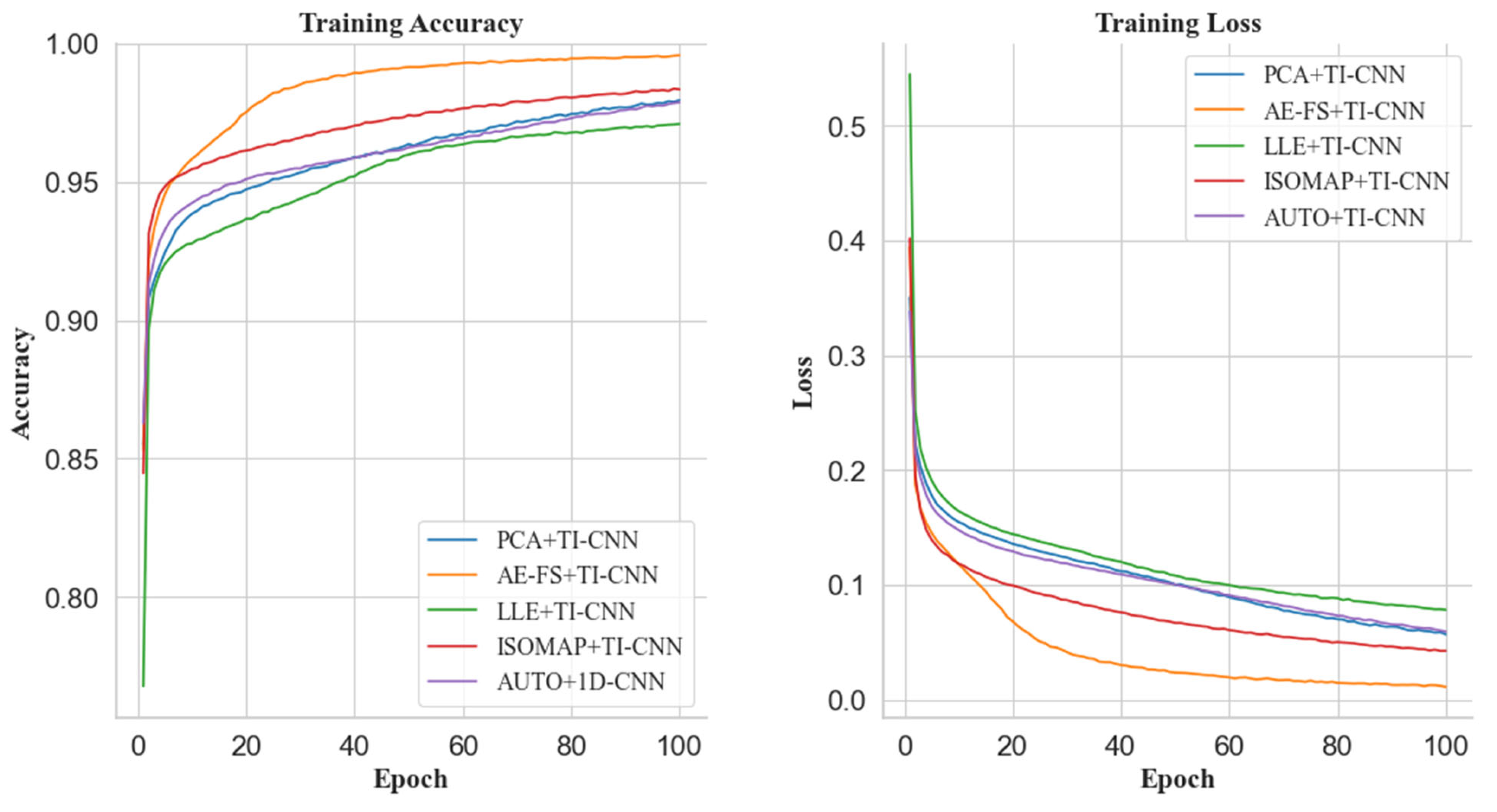
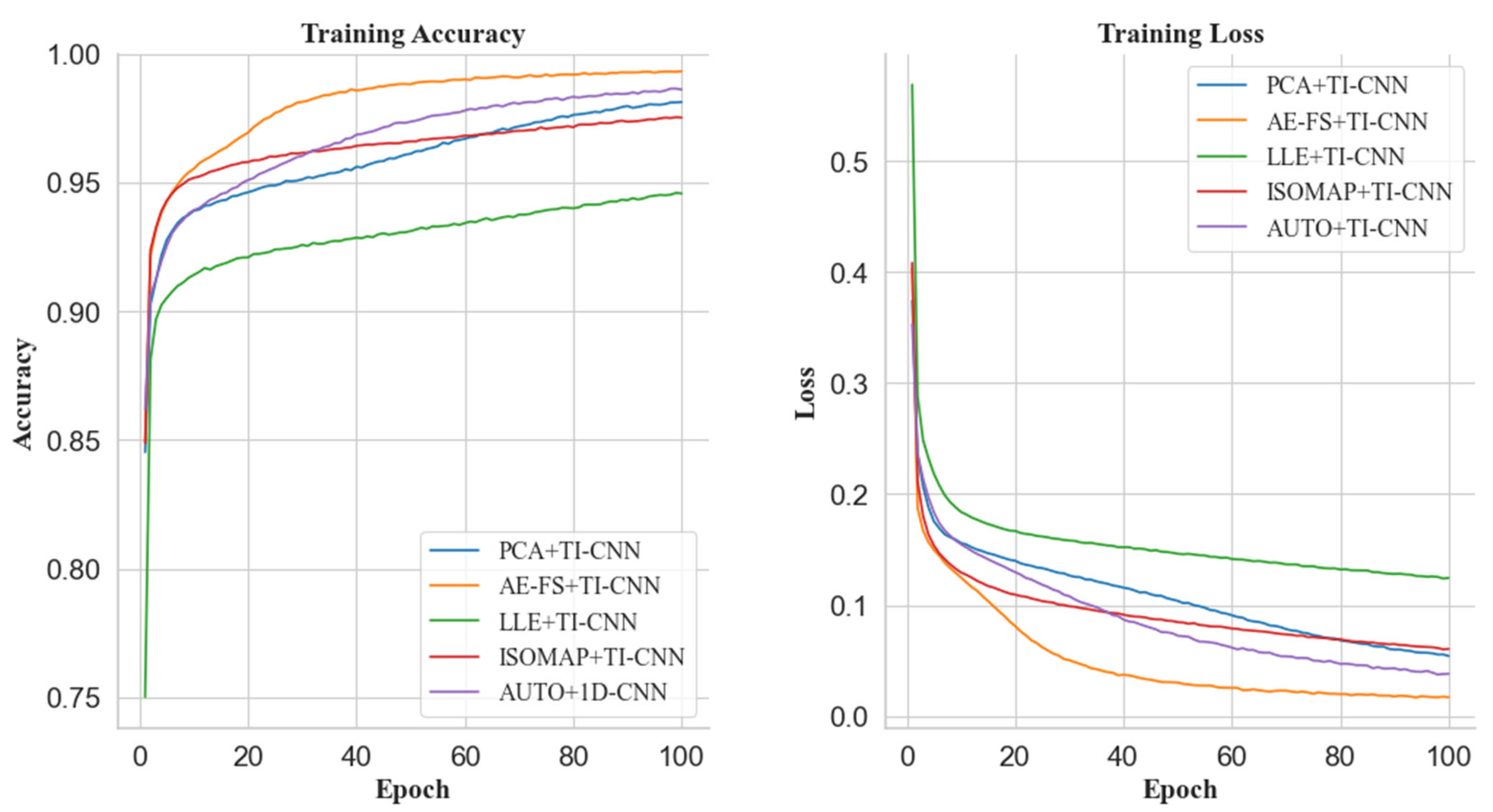
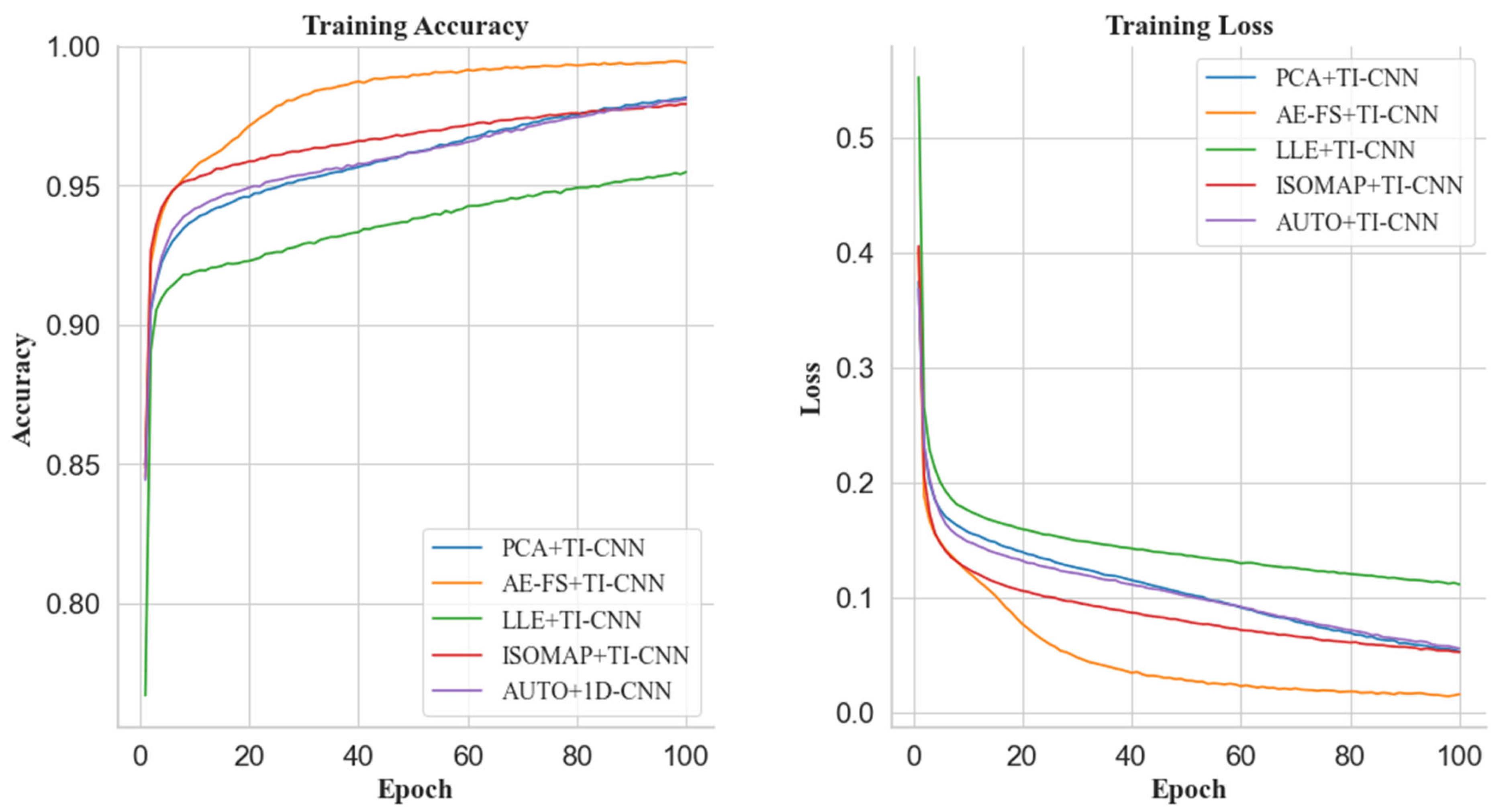
Regarding the training accuracy of the training model, the AE-FS dimensionality reduction dataset shows apparent advantages in the training process. For example, when the dataset is reduced to 25 dimensions, the feature reduction rate is 10.8% (as shown in Figure 7). The AE-FS+TI-CNN model first reaches the fitting state at the beginning of training and reaches the highest at the end of training. The training accuracy rate is about 98%. 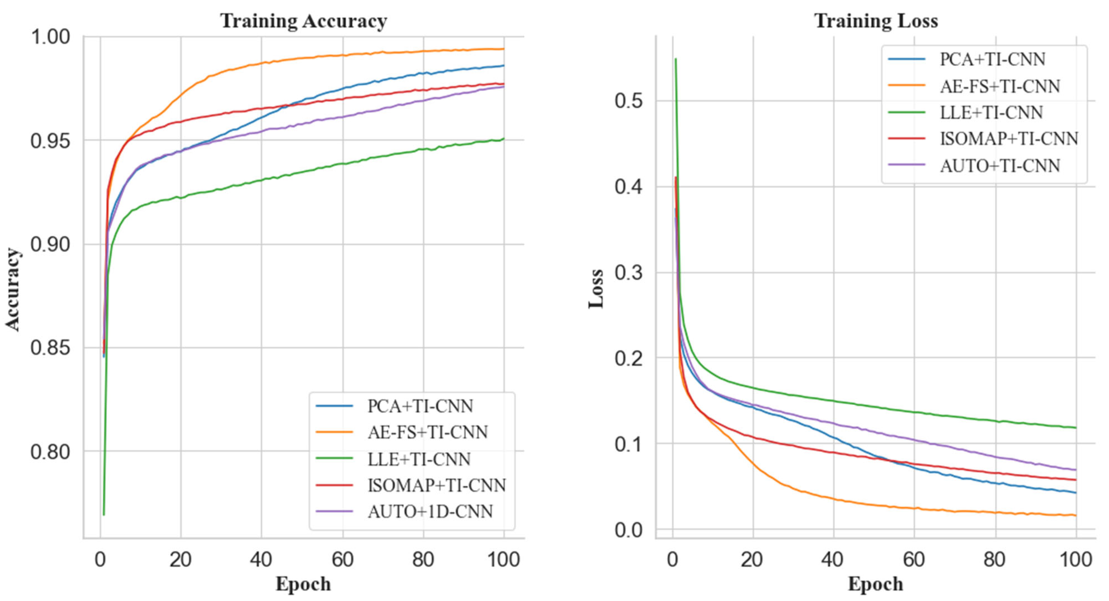Similarly, when the dataset is reduced to 20 dimensions, the feature reduction rate is 28.6% (as shown in Figure 8). The FS+TI-CNN model has a clear advantage in training accuracy, which is higher than that of the PCA+TI-CNN model by 2.5%. In addition, when the dataset is reduced to 18 dimensions, the feature reduction rate is 35.7% (as shown in Figure 9), and the training accuracy of the FS+TI-CNN model is 0.8% higher than that of the PCA+TI-CNN model. Finally, when the dataset is reduced to 16 dimensions, the feature reduction rate is about 42.9% (as shown in Figure 10). The AE-FS+TI-CNN model also has a clear advantage in training accuracy. Compared with AUTO+TI-CNN the model is 0.5% higher. In summary, the AE-FS dimensionality reduction method shows excellent performance and advantages when dealing with high-dimensional datasets, and its model quickly reaches the fitting state during the training process and achieves the highest training accuracy at the end of the training.

Regarding model training loss rate, when the dataset is reduced to 25 dimensions (as shown in Figure 7), the AE-FS+TI-CNN model performs best, which is 3% lower than the ISOMAP+TI-CNN model training loss rate. Meanwhile, the loss rate of the LLE+TI-CNN model converges the slowest. When the dataset is reduced to 20 dimensions (as shown in Figure 8), the loss rate of the AE-FS+TI-CNN model is 4% lower than that of the ISOMAP+TI-CNN model, and the loss rate of the LLE+TI-CNN model also converges the slowest. When the dataset is reduced to 18 and 16 dimensions (as shown in Figure 9 and Figure 10), the loss rate of the AE-FS+TI-CNN model also performs best. Compared with the PCA+TI-CNN model and AUTO+, the TI-CNN model is about 2.5% and 2% lower, respectively, and the loss rate convergence of the LLE+TI-CNN model is still the slowest.

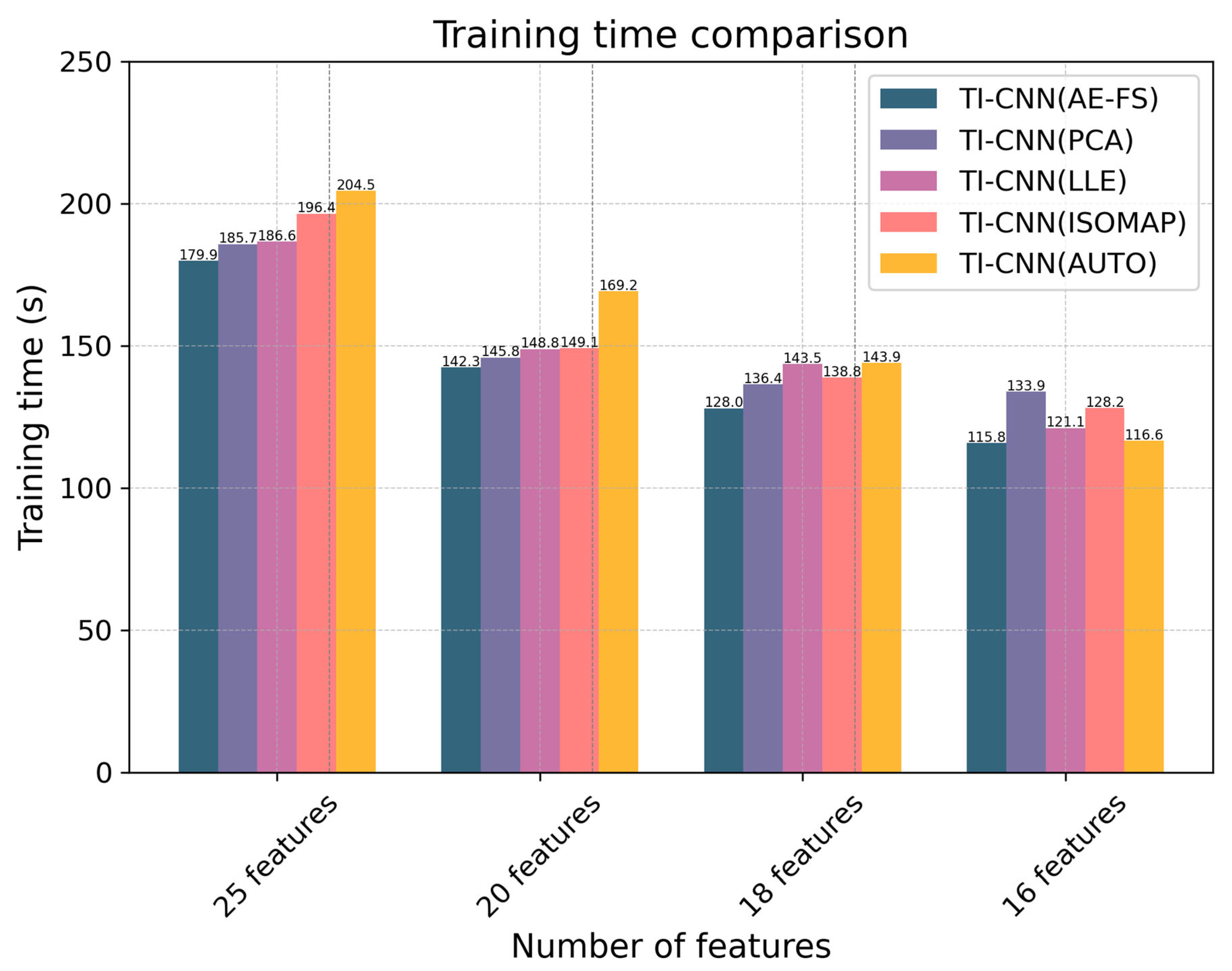
Regarding model training time, the experimental results are shown in Figure 11. In general, the less dimensionality of the dataset, the shorter the training time of the model. When reducing the dataset to 25 dimensions, the AUTO+TI-CNN model exhibits the longest training time of approximately 204.5 s, whereas the AE-FS+TI-CNN model shows the shortest training time of about 179.9 s. The difference between the two is approximately 25 s, with a relative difference rate of around 12.2%. When the dataset is reduced to 20 dimensions, the AUTO+TI-CNN model requires the longest training time, about 169.2 s; the AE-FS+TI-CNN model requires the shortest training time, about 142.3 s. Similarly, when the dataset is reduced to 18 dimensions, the AUTO+TI-CNN model requires the longest training time, about 143.9 s, and the AE-FS+TI-CNN model requires the shortest training time, about 128 s. Furthermore, when the dataset is reduced to 16 dimensions, the training time required for the AUTO+TI-CNN model is the shortest, which is 115.8 s. Therefore, it can be concluded that the AE-FS dimensionality reduction method can significantly reduce the training time of the model while maintaining a high training accuracy.

From

Table 4. Comprehensive comparison of different dimensionality reduction methods.

Data Dimension	Method	Data Reduction Time (s)	Model Training Time (s)	Accuracy
25	PCA	3.2	185.7	97.2%
	LLE	111.4	186.6	96.7%
	ISOMAP	155.6	194.6	97.0%
	AUTO	6.2	204.5	97.1%
	AE_FS	10.1	179.9	98.8%
20	PCA	3.2	145.8	97.1%
	LLE	111.6	148.8	95.3%
	ISOMAP	157.2	149.1	96.8%
	AUTO	5.7	169.2	97.2%
	AE_FS	10.3	142.3	98.6%
18	PCA	3.2	136.4	96.9%
	LLE	113.4	143.5	94.9%
	ISOMAP	158.0	138.8	96.5%
	AUTO	5.7	143.9	97.8%
	AE_FS	9.8	128	98.5%
16	PCA	3.2	133.9	96.5%
	LLE	113.1	121.1	94.5%
	ISOMAP	156.6	128.2	96.7%
	AUTO	5.6	116.6	97.7%
	AE_FS	10.1	115.8	98.3%

, we implemented five different dimensionality reduction techniques to decrease the number of dimensions in the dataset to 25, 20, 18, and 16. The dimension re-duction time for LLE and ISOMAP is considerably longer compared to PCA, AUTO, and AE_FS. This is because LLE and ISOMAP take into account more local information and the relationships between data points during the calculation process, resulting in increased dimension reduction time. AE_FS takes slightly longer than PCA and AUTO for data dimensionality reduction, but it outperforms them in terms of model training time and classification accuracy. It is important to note that the data dimensionality reduction process can be performed offline, which helps mitigate the impact of dimensionality re-duction time on the overall model performance. Therefore, considering data dimension reduction time, model training time, and classification accuracy, it is evident that AE-FSS still holds significant advantages over other methods. In practical applications, AE-FSS offers the dual advantages of efficiency and accuracy in data processing.

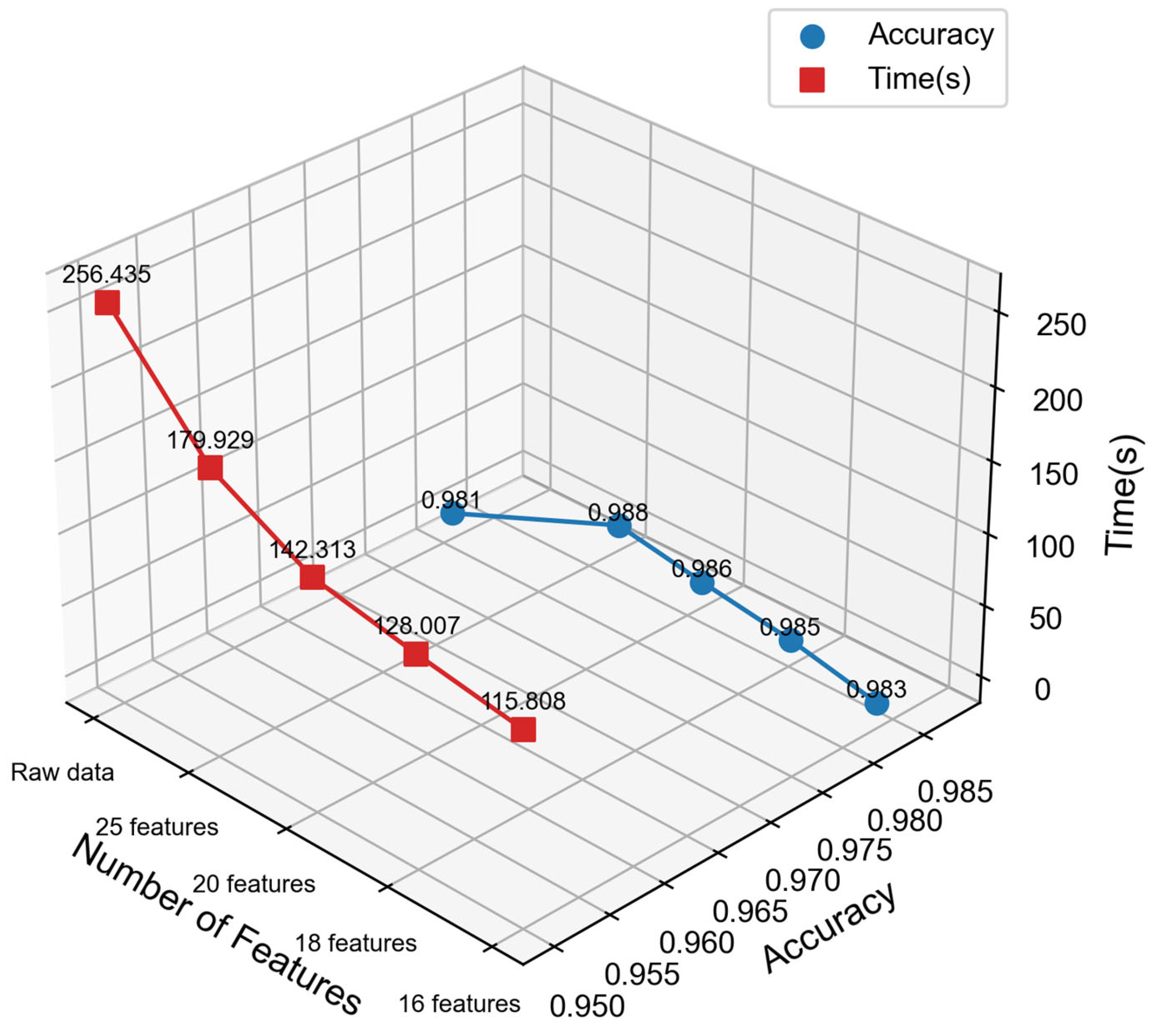
According to the results in Figure 12, it can be observed that the training time of the model is significantly reduced through the AE-FS dimensionality reduction dataset. Especially when the dataset is reduced to 16 dimensions, the time reduction is the most significant, with a drop of up to 54.3%. At the same time, the classification accuracy of the AE-FS+TI-CNN model is the same as that of the original dataset, the highest training accuracy is 98.8%, and the lowest is 98.3%. Compared with the original dataset. The classification accuracy of the AE-FS+TI-CNN model increased by about 0.7% and 0.2%. Therefore, it shows that dimensionality reduction through AE-FS not only fully preserves the key features of the dataset, but also dramatically reduces the training time of the model.

4.4.2. Comparison of AE-DTI with Other Methods

This section examines the classification performance and effectiveness of four models. These models include the following: Lashkari et al. [21] utilized time-based features extracted from 15-s Tor traffic to train a random forest model; Yan, H et al. [29] employed sliding time windows to segment network traffic and calculated the relative entropy of traffic within the time window to identify Tor traffic; Haoyu Ma et al. [30] proposed a deep-learning-based scheme for detecting dark web traffic (Tor traffic); and this paper presents a darknet traffic identification method based on autoencoder (AE-DTI). All of these models were trained on the ISCXTor dataset.

The experimental results are presented in

Table 5. Performance of different dark network traffic identification methods.

Method	Accuracy	Pre	Recall
Lashkari et al. [21]	-	84.3%	83.8%
Yan, H et al. [29]	91%	91%	91%
Haoyu Ma et al. [30]	-	95.5%	-
AE-DTI (25 features)	98.8%	98.6%	98.7%
AE-DTI (20 features)	98.6%	98.5%	98.7%
AE-DTI (18 features)	98.5%	98.5%	98.5%
AE-DTI (16 features)	98.3%	98.3%	98.4%

. With the exception of Lashkari et al.’s method, the accuracy of the other methods exceeds 90%, and the accuracy of AE-DTI surpasses 98%. Particularly, when the dataset is reduced to 16 dimensions by AE-FS, AE-DTI requires minimal features for training. However, AE-DTI performs better than other methods in every evaluation index. Consequently, AE-DTI not only enhances the efficiency of traffic identification but also significantly improves classification accuracy. This is of substantial importance in enhancing the efficiency and accuracy of traffic identification, and it can serve as a valuable reference for research and practical applications in related fields.

4.4.3. AE-DTI Generalization Experiment

To verify the generalization of AE-DTI, this paper conducts comparative experiments on the CSE-CIC-IDS2018 dataset and the CIC-Darknet2020 dataset. Various dimensionality reduction methods (PCA, LLE, ISOMAP, autoencoder, and AE-FS) were used to reduce the dimensionality of the two datasets to 49 and 64 dimensions, and then model training and classification experiments were performed, respectively. The experimental results are shown in

Table 6. Experimental classification results with a feature number of 49.

Dataset	Algorithm	Acc	F1	Pre	Recall
CSE-CIC-IDS2018	AE-FS	96.6%	96.3%	96.1%	96.6%
	AUTO	95.8%	95.8%	95.8%	95.7%
	ISOMAP	95.9%	96.1%	96.2%	95.9%
	LLE	96.1%	96.1%	96.1%	96.1%
	PCA	95.1%	95.3%	95.5%	95.1%
CIC-Darknet2020	AE-FS	87.1%	86.9%	86.8%	87.1%
	AUTO	85.8%	85.3%	85%	85.8%
	ISOMAP	84.0%	84.2%	84.4%	84%
	LLE	85.1%	84.4%	83.6%	85.1%
	PCA	85.7%	85.3%	84.9%	85.7%

and

Table 7. Experimental classification results with a feature number of 64.

Dataset	Algorithm	Acc	F1	Pre	Recall
CSE-CIC-IDS2018	AE-FS	98.8%	98.8%	98.9%	98.8%
	AUTO	98.3%	98.4%	98.4%	98.3%
	ISOMAP	95.8%	96%	96%	95.8%
	LLE	96.8%	96.8%	96.9%	96.8%
	PCA	94.9%	95.2%	95.4%	95%
CIC-Darknet2020	AE-FS	89.5%	89.6%	89.6%	89.5%
	AUTO	85.8%	85.3%	85%	85.8%
	ISOMAP	83.8%	84.2%	84.5%	83.8%
	LLE	84.8%	84%	83.3%	84.8%
	PCA	85.4%	84.9%	84.5%	85.4%

.

According to the results in Table 6, when the dataset is downscaled to 49 dimensions, for in the CSE-CIC-IDS2018 dataset, the model trained by the dataset downscaled by AE-FS outperforms the other methods, with Acc, F1 value, and Recall improving by 1.5%, 0.8%, and 1.5% compared with PCA downscaling. It is slightly lower than the model trained on the dataset via ISOMAP dimensionality reduction in Pre, with a difference of about 0.1%. For the CIC-Darknet2020 dataset, the model trained on the dataset downscaled by AE-FS outperforms the other methods in Acc, Pre, F1 value, and Recall. At the same time, it is worth noting that for unbalanced datasets such as CIC-Darknet2020, AE-IDT still shows good classification results.

According to the results in Table 7, when the dataset is downscaled to 64 dimensions, for the CSE-CIC-IDS2018 dataset, the models trained on the dataset downscaled by AE-FS outperform the other methods, with the Acc, F1 value, Pre, and Recall improving by 3.9%, 3.6%, 3.5%, and 3.8% compared with PCA downscaling. For the CIC-Darknet2020 dataset, the models trained on the dataset with AE-FS dimensionality reduction also outperformed the other methods in terms of Acc, F1 value, Pre, and Recall. At the same time, it is worth noting that for unbalanced datasets such as CIC-Darknet2020, AE-IDT still shows good classification results.

5. Conclusions

The traffic identification method AE-DTI based on an autoencoder proposed in this paper has apparent advantages in improving identification efficiency and classification accuracy. First of all, through the multi-dimensional comparative experiments on the ISCXTor2016 dataset, the results show that the dimensionality reduction in the dataset through AE-FS can not only fully retain the key features of the original dataset but also significantly reduce the training time of the model. At the same time, comparing AE-DTI with other model methods, AE-DTI shows obvious advantages in classification accuracy. Then, by verifying the generalization of AE-DTI on the CSE-CIC-IDS2018 and CIC-Darknet2020 datasets, AE-DTI still has obvious advantages.

Therefore, the AE-DTI method proposed in this paper shows good performance and feasibility in darknet traffic identification. It can not only effectively identify darknet traffic but also improve the training efficiency and classification accuracy of the model. This is of great significance to the research and application in the field of network security and provides valuable enlightenment for further improving and optimizing the darknet traffic identification method.