Predicting Models for Local Sedimentary Basin Effect Using a Convolutional Neural Network

Abstract

Although the numerical models can estimate the significant influence of local site conditions on the seismic propagation characteristics near the surface in many studies, they cannot feasibly predict the seismic ground motion amplification in regular engineering practice or earthquake hazard assessment due to the high computational cost and their complex implementation. In this paper, the scattering problem of trapezoidal sedimentary basins, one of the representatives of local complex sites with a relatively small model size, and simplified by practice in this type of study, was selected as the basin model. A series of standard basin models were built to quantify the relationship between the site condition parameters and the site amplification parameters (the peak ground acceleration and the hazard location). In addition, the factors that influence seismic ground motion amplification, such as the basin shape ratio, the soil depth, the basin edge dip angle, the ratio of shear wave velocity between the bedrock and the soil layer, the damping coefficient, and the fundamental frequency, were selected to investigate the sensitivity. A convolutional neural network (CNN) algorithm based on deep learning replacing traditional recursive algorithms was explored to establish a prediction model of basin amplification characteristics. By the Bayesian optimization method, the structural parameters of the CNN predicting model were selected to improve the accuracy of the prediction model. The results show that the optimized CNN models could predict the amplification characteristics of the basin better than the un-optimized CNN models. Three prediction models were established with the site condition parameters as the input parameters and their output parameters were the maximum amplification value of the peak ground acceleration (PGA), the hazard location, and their combination for each basin. To analyze the CNN’s prediction ability, each CNN model used about 80% of the data from the seismic model repose results for training and the remaining data (20%) for testing. By comparing the CNN prediction results with the FE simulation results, the accuracy and rationality of each prediction model were studied. The results show that, compared to a single numerical model, the CNN prediction results of the site amplification features could be quickly obtained by inputting the relevant parameters. Compared to recursive class models, the established CNN prediction model can directly establish the relationships among multiple input and multiple output parameters. A comparison of the three kinds of CNN models shows that the prediction accuracy of the joint parameter model was slightly lower than that of the two single-output models.

1. Introduction

As the propagation medium of seismic waves and the ground of building structures, a local site will significantly affect the ground motion. Previous investigations have recorded relatively serious earthquake damages in a basin, which is a special site, and its influence on ground motion has been studied. The basin effect includes the selective amplification of long-period ground motion by the soft soil layer and the abnormal amplification of the basin edge [1,2]. These special amplifying characteristics of ground motion are some of the representative parameters to measure the ground motion amplification of the basin, as well as the amplification of the peak of the ground acceleration. Therefore, it is of great importance to predict the peak amplification and location of the ground motion acceleration in the basin to evaluate the safety of many high-rise buildings located in basins in inner cities.

The influence analysis of sedimentary basins on ground motion is theoretically a problem of two-dimensional (2D) or three-dimensional (3D) dynamic response analysis. More efficient and flexible numerical simulation methods are mostly adopted, and detailed site data are needed to establish a more accurate 3D computational model. With the development of computing technology, numerical methods have overcome the challenge of computational accuracy and stability, and have achieved great development and wide application. In terms of computing software, general commercial finite element software is widely used in the field of research and design currently, including ANSYS, ABAQUS, FLAC, LS-DYNA, ADINA, Marc, etc. [3], all of which have perfect modeling, solving, and post-processing functions. In view of the physical characteristics of basins, many scholars have improved the level of existing special analysis methods from many aspects and perspectives, and have developed a series of special analysis software, such as CESAR-LCPC [4] and AHNSE [5]. Based on the current analysis techniques, complex 2D and 3D computational models reflecting as many factors as possible have been established to reflect the detailed characteristics of the sedimentary basin geological structure and focal information, etc., and different numerical methods are used to reproduce the ground motion characteristics. Riga et al. [6] conducted extensive numerical analysis on the linear viscoelastic response of homogeneous sedimentary basins and explored the potential additional influence of sediment heterogeneity and nonlinearity on the weighting coefficient through a finite element model developed in ABAQUS. Bazyar et al. [7] used the scaled boundary finite element method to directly deal with irregular phenomena in the time domain, and discuss the scattering and amplification of seismic waves under topographic and geological conditions. Meza-Fajardo et al. [8] reconstructed the engineering geological model of the alluvial valley and evaluated the local response of the ground motion in terms of surface propagation, amplification function, and cumulative kinetic energy by using a 2D finite element numerical simulation method.

The basin effect is often caused by the combined action of many factors, such as subsurface media and irregular site geometries. The 2D characteristics of the variation of heterogeneous media in the basin have been proven to change the nature of seismic wave propagation from deep underground to the surface. The results show that for sedimentary basins with significant amplification characteristics, it is necessary to reflect the joint influence of the spatial geometric characteristics and the physical characteristics of the sedimentary soil layer. Therefore, on the basis of qualitative research, how to quantitatively analyze the amplification effect of different factors on the basin, how to reasonably evaluate the basin effect, and how to scientifically predict the ground motion are the key problems to be solved in engineering applications. However, due to the complexity of the structure and soil of real basins, only approximate or simplified models can be used, so it is necessary to study the laws of the amplification mechanisms of different types of basins, to establish the relationship between the parameters and the amplification characteristics, and to improve the existing methods, taking into account the site’s effect. In order to analyze the significance of different factors on the basin amplification effect, based on the reasonably simplified standard basin model, the influence of each factor on the ground motion is analyzed by changing the parameters of the numerical simulation method. Moczo et al. [9], based on the numerical modeling of sedimentary basins with different dimensions, studied in detail the relationship between the ground motion response of surface stations and their own geometry, the quality factor of the soil layer medium, and the impedance ratio by changing the depth-to-width ratio of the model. Liang et al. [10] popularized the indirect boundary integral equation method to solve the scattering of plane waves and SV waves by a mountainous terrain in a half-space and found that the scattering characteristics of plane waves in a mountainous terrain were greatly related to the incident angle, frequency, and characteristics of the mountainous medium. The comparison of different simplified analysis models provides a basis for describing a site’s response reliably using as few parameters as possible. Anquez et al. [11] established a basin model of the lower Vale valley in France and studied the influence of geometric model simplification on wave propagation by using the discontinuous Galerkin finite element method. Raptakis et al. [12,13] calculated the seismic response of a series of 2D Greek Volvi basin models with different levels of detail in order to capture the nature of their seismic response. It is a representative research idea to use a simplified model that reflects the characteristics of ground motion amplification, rather than using a complex real sedimentation basin model.

The influence of the site effect on ground motion can be roughly estimated using ground motion prediction equations, which are primarily based on the observation data obtained from existing stations. These equations extract relevant parameters and reflect the influence of the site effect through simple regression. However, as one of the typical local complex sites, the small- and medium-sized basins are characterized by the undulating shape of the bedrock at the bottom, soil properties, lateral inhomogeneity, and surface topography, which are all factors leading to abnormal ground motion [14], and have complex seismic wave propagation characteristics. Because the observed data are not rich enough and the relative scale is small, the effect of the regression prediction can hardly reflect the local change characteristics of the ground motion. How to reasonably reflect the influence of local site effect in the ground motion prediction of the basin is a problem that needs to be solved to ensure the project’s safety. In recent years, with the popularity of artificial intelligence, machine learning has been increasingly applied to the field of civil engineering due to its ability to directly acquire information from data, without assuming the obedience law or internal relationship between data or parameters in advance. For example, in the area of automatic diagnosis of concrete arch beam damage, a method based on optimized deep stacked self-encoders and multi-sensor fusion is proposed, which is important in terms of reducing labor costs and risks [15]. An approach based on an improved bird flocking algorithm and 2D convolutional neural networks is used to assess the torsional capacity of reinforced concrete beams. Accurate and fast torsional capacity assessment is achieved through optimal feature selection and model training [16]. In the area of earthquake engineering, SunyulKim et al. [17] develop a ground motion amplification model based on three machine learning techniques (i.e., random forest, gradient boosting, and artificial neural network) using the record database of KiK-net site in Japan, and propose that machine learning is superior to the regression method. The data-driven method based on numerical simulation is widely used in machine learning to address the limitation of the lack of real observational data. Karimi et al. [14] adopt the fuzzy logic method and flexible interference rules to eliminate the uncertainty caused by the deviation of local data and established the peak ground acceleration prediction model of the Iranian plateau, which can also be improved and updated according to the newly added data. Mir et al. [18] used a machine learning-based ensemble model to predict radon time series anomalies in earthquake likelihood. However, the traditional artificial neural network also has some shortcomings, such as slow convergence speed, local extreme value, low quantization accuracy, and data over-fitting. In addition, with the continuous expansion of the data set, the low computing speed of the traditional neural network similar to backpropagation neural network can no longer meet the computing needs. CNN has attracted wide attention due to its powerful feature learning and recognition ability. It is not a simple memory superposition but a comprehensive evaluation of training data, which has a certain degree of fault tolerance and has important application value. Based on this, this paper aims to establish an accurate and efficient model for predicting basin amplification characteristics using CNN.

Considering that the one-dimensional (1D) basin model will underestimate the amplification value, and the computational cost of the 3D model is high and time-consuming, we used the simplified standard basin model and the commercial finite element software ABAQUS (version 6.14) to establish a series of 2D basin models, and relied on its PYTHON (version 2.7) interface for secondary development to realize batch modeling to quickly build the CNN sample database. In order to study the site effect, the key parameters affecting the basin effect were taken as the CNN input, and the basin amplification characteristics represented by the peak value of the amplification coefficient and the hazard location were taken as the CNN output to establish the prediction model. To improve the accuracy of prediction, this paper built a CNN model combined with a Bayesian optimization algorithm, analyzed the sensitivity of input parameters, optimized the input parameters to build the optimal CNN model, and used the CNN model to identify the amplification characteristics of basins. Finally, a reasonable surface amplification prediction model for local sedimentary basins was established, which achieved the purpose of rapid surface amplification prediction and provided a rapid and effective prediction method for the next step of seismic hazard assessment and seismic design.

2. Method

2.1. Overall Research Idea

In this paper, the characteristics of typical basin ground motion amplification were obtained by numerical analysis methods, including the maximum amplification factor and the hazard location (the location of the maximum value). A large number of basin surface response data were simulated by an automatic basin analysis model construction method. Then, the geometric shape of the basin and the material parameters of each soil layer were used as the prediction model of the CNN input, and the peak ground acceleration and the hazard location were used as the CNN output, and the process is shown in Figure 1. The CNN can automatically extract the basin ground motion amplification characteristics from these data, which does not require complex modeling and time-consuming computation as traditional numerical simulation methods, and is given for engineering applications. The method was summarized below:

Figure 1. Numerical analysis process.

(1)

The shape and material parameters of the basins were modified to establish a basin model database;

(2)

The finite element method (FEM) was used to calculate the amplification factor and determine the hazard location in batches;

(3)

The generated database was used to train the CNN;

(4)

The trained CNN was tested and its predictions were compared with the FEM results.

2.2. Numerical Modeling for Ground Motions of a Basin

Based on the finite element method (FEM), this paper used commercial finite element software ABAQUS [19] to calculate the basin ground motion response. The seismic response of a 2D local complex site is a problem of wave propagation in the infinite domain. In practice, considering that the amount of computation usually intercepts the finite domain and then sets a special artificial boundary to absorb the external wave to simulate the effect of the infinite domain, a damping unit can be set at the model boundary as a viscous boundary in ABAQUS [19] to reasonably realize the wave absorption. At the same time, the seismic input also needs to be converted into equivalent nodal force and applied as the load at the boundary in ABAQUS. At present, ABAQUS software cannot directly add artificial boundary and seismic input through the interactive interface, which needs to be realized by modifying the keywords in the INPUT file. The Python interface of ABAQUS was used to write scripts to automatically modify the input files to achieve the artificial boundary and equivalent nodal force. After ABAQUS CAE modeling, the program was executed, which consisted of five steps:

(1)

The geometry and media information of the basin profiles was read;

(2)

The cell grid size was set to identify the boundary node and store the information;

(3)

The boundary node damping coefficient was calculated;

(4)

The seismic acceleration time history was read to calculate the equivalent node forces;

(5)

The damping coefficients were associated with the equivalent nodal forces to the corresponding boundary nodes.

The damping coefficient of Step (3) was calculated from Equations (1) and (2) using the following equation:

$$C_N=\rho {\nu }_P·A$$

(1)

$$C_T=\rho {\nu }_S·A$$

(2)

where $N$ is the normal direction, $T$ is the tangential direction, ρ is the density, ${\nu }_P$ is the compressional (P) wave velocity, ${\nu }_S$ is the shear wave velocity, and $A$ is the cell area. As shown in Figure 2, the equivalent nodal forces of Step (4) were calculated according to the physical and mechanical parameters of the bedrock and the time history of the incident seismic wave, and the equation was as follows:

$$\mathsf{\Delta }{t}_1=\frac{H_1}{v_s}$$

(3)

$$\mathsf{\Delta }{t}_2=\frac{(2H-H_1)}{v_s}$$

(4)

$$\mathrm{Swave}: F_x^{-y}=A\rho v_s{\dot{u}}_s(t)$$

(5)

$$\mathrm{Swave}: F_y^{-x}(t)=-F_y^{+x}(t)=A\rho v_s[{\dot{u}}_s(t-\Delta t_1)-{\dot{u}}_s(t-\Delta t_2)]$$

(6)

where the subscript $x$ or $y$ is the direction of the force applied to the node; the superscript $x$ or $y$ is the direction of the external normal; $\Delta t_1$ and $\Delta t_2$ are the delay times of the incident and reflected waves at the boundary, respectively. H is the height from the bottom boundary to the surface, and H₁ is the height from the bottom boundary to the calculation node.

Figure 2. Schematic illustration of finite element main grid coupling to boundary grids by viscous dashpots and equivalent nodal forces.

2.3. Summary of 1D CNN

The basic structure of the CNN model usually includes an input layer, convolution layers, a fully connected layer, and an output layer. The input data were transferred through a series of layers (three convolution layers, activation function, and loss function). Finally, the mapping calculation obtained the amplification factor. Specifically, the input of the 1D CNN was either a 1 × N or an N × 1 array. As shown in Figure 3, an N × 1 array was passed through a series of convolution layers and the fully connected layer. Then, the amplification factors for the local ground motion were obtained in the output layer.

Figure 3. The 1D CNN model.

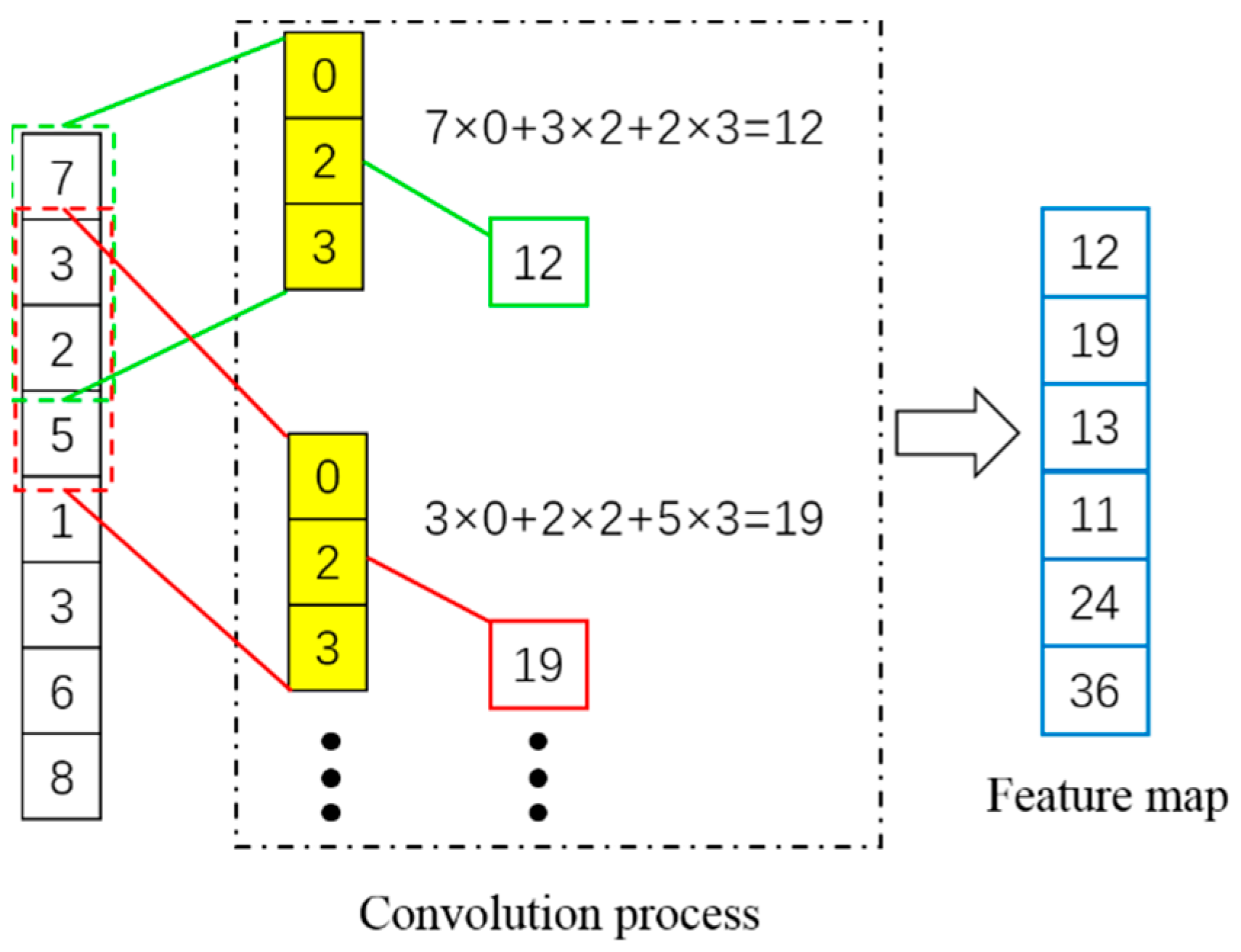
The function of the convolution layers was to extract features from the input data. As shown in Figure 4, the convolution process was to multiply each element in the convolution kernel (e.g., yellow box) by the corresponding element in a subregion (e.g., green or red dotted box) of the convolution layer input data, and summing the products to obtain an element in the feature map. Each time, the sub-region was moved down by one step, and the process was repeated until all elements of the input data were involved. Finally, the convolution operation formed a new array (i.e., the feature map).

Figure 4. Convolution process.

The activation function introduces nonlinearity so that the CNN can approximate any nonlinear function arbitrarily to achieve better learning capabilities [20]. Commonly used activation functions include the Sigmoid, Tanh, ReLU (rectified linear unit), and LeakyReLU functions [21], as shown in Figure 5. The ReLU activation function and LeakyReLU activation function converge faster compared to the Sigmoid activation function and Tanh activation function [22]. The ReLU activation function has an output of 0 when x < 0, which causes zero gradients for negative x, making the neurons no longer activated during training, and some effective features in the data are blocked. The LeakyReLU activation function is an improved version of the ReLU activation function, which inherits the advantages of the ReLU activation function, and retains a smaller slope in the negative region [23]. Therefore, in this paper, we adopted the LeakyReLU activation function.

Figure 5. Activation function: (a) Sigmoid; (b) Tanh; (c) ReLU; (d) LeakyReLU.

The fully connected layer was usually at the end of the CNN, which can collect the extracted features together (integration features) and usually need to define a loss function before the output layer. The loss function is to calculate the difference between the prediction result and the actual value for the CNN at each iteration, so as to guide the next network training to proceed in the right direction (less error).

3. Basin DATABASE

3.1. Generation Method of Basin Models

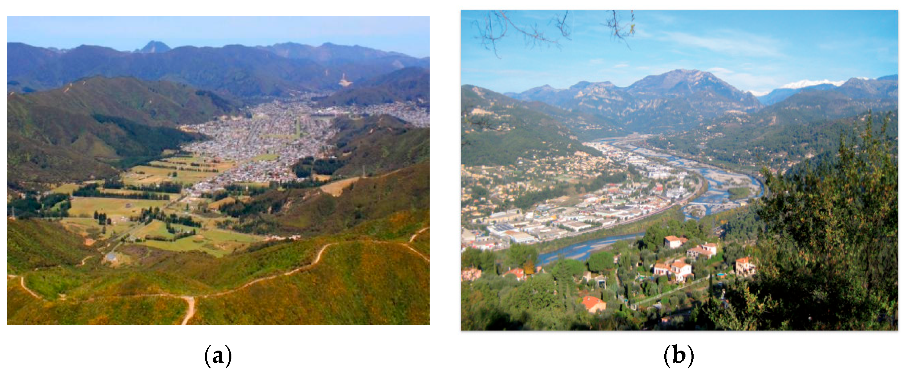
As shown in Figure 6, the flat topography in the interior of the basin provided a livable environment for human life, but the surrounding raised topography and the deep soil layer covering it had a significant amplifying effect on the ground motion. In order to study the basin amplification law, the real basin was usually simplified into a standard basin structure model [12]. According to the significant geometric characteristics of the flat center and the steep edge of the basin, a simplified 2D basin model of an “inverted trapezoid” was established, as shown in Figure 7.

Figure 6. Illustration of the site of a basin. (a) Lower Hutt valley basin in Wellington, New Zealand. (b) Lower Var valley basin in Nice, France.

Figure 7. Simplified diagram of the standard basin.

The aim of this study is to perform a comprehensive analysis of the seismic response of a typical 2D basin model with a wide range of geometric and material properties in order to study the response of the basin surface in relation to the basin geometry (width, thickness and slope angle of the lateral boundaries) and soil dynamic properties (shear and compression wave velocities, soil density, and attenuation), and in particular, to predict the potential hazard in the local basin area by determining the amplification characteristics of the peaks and the hazard location.

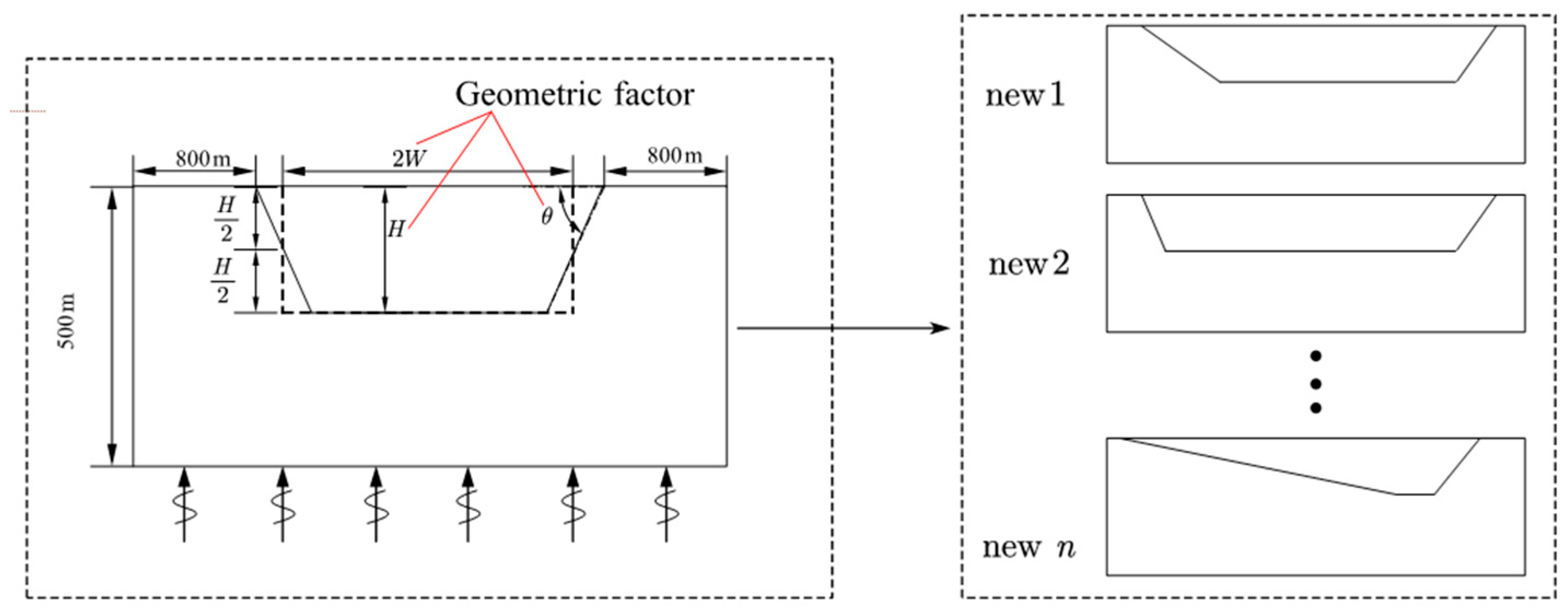
The research showed that the amplification characteristics of 2D compared to 1D were mainly due to the influence of surface waves and 2D resonance. The factors influencing the characteristics were mainly shape ratio and wave velocity ratio. These represented the influence of geometry and medium properties in site conditions. As shown in Figure 8, the shape ratio was defined as H/2W where 2W was the total width over which the sediment thickness was more than half of its maximum value. The wave velocity contrast $C_V$ was defined as the ratio of the soil shear wave velocity to the bedrock shear wave velocity. The parameters related to the basin amplification effect were comprehensively considered to construct a series of numerical models for the basin surface seismic response analysis by varying the geometric parameters: thickness, shape ratio, edge dip angle (shown in Figure 8), and soil medium parameters such as shear wave velocity, density, Poisson’s ratio, quality factor, damping ratio, etc.

Figure 8. Sample amplification process.

In order to investigate the sensitivity of the 2D seismic response of trapezoidal basins to various parameters related to basin geometry and sediment properties, an extensive numerical analysis of homogeneous soil basins with linear viscoelastic soil behavior was carried out. The parameters and models were selected mainly with reference to the parameter ranges of the literature [24] while considering the characteristics of the physical parameters of the site as specified in the Chinese Seismic Code, and similar works were found in the literature [25,26,27]. Homogeneity and viscoelastic behavior were chosen as reference assumptions for the numerical models, which is a common practice in such studies [24]. The surface ground motion was simulated in batch by the finite element software ABAQUS, and the specific analysis process was described in the previous subsection, similar simulation processes were found in the literature [25,27,28]. This paper focused on the amplification characteristics of small and medium-sized basins, which span less than 3000 m. The influence of incident angle and incident wave frequency was not considered in this study. In order to reduce boundary errors, the bedrock was set laterally to 800 m from either side of the basin, and the overall height of the model was unified as 500 m. The range of soil properties in the basin was controlled within a reasonable variation, so as to satisfy the richness of the basin geometry and medium parameters. Based on the adjustment of basin shape and physical–mechanical parameters, a large number of basin models were formed. Table 1 summarizes the main geometric and dynamic properties of all the models, which refer to four groups of shape ratios, each corresponding to two depth cases of 200 m and 300 m, and a total of eight combinations, with limit angles for the dip angle under each combination, generating a total of 756 basin models, including the asymmetric case where the dip angle is unequal on both sides.

Table 1. Modification rules of physical and mechanical parameters of soil layers.

Depth (m)	Shape Ratios	Dip Angle (°)	${\mathit{V}}_{\mathit{s}} (\mathbf{m}/\mathbf{s})$
200/300	0.15	10/20/30/45/60/75/90	200/250/300/ 400/500/600
	0.2	20/30/45/60/80
	0.3	30/45/60/80
	0.4	30/45/60/80

Both sides of the basin were bedrock with a shear wave velocity of 1500 m/s, density of 2200 kg/m³, and the ratio of Poisson of 0.2. In the soil media properties, the ratio of Poisson was 0.3 for the average value of all soil types and the shear wave velocity was selected between 200 m/s and 600 m/s to cover most of the engineering site conditions [24]. The density was estimated from Equation (7) according to the shear wave velocity [29]. The p wave velocity was converted according to the relationship between the transverse wave velocity and the ratio of Poisson in Equation (8). In the equation, ρ is the density of the soil layer, $\upsilon$ is the ratio of Poisson, $V_s$ and $V_p$ are shear wave velocity and longitudinal wave velocity, respectively.

$$\rho =0.6V_s^{0.183}$$

(7)

$$V_p=\sqrt{\frac{2-2\upsilon }{1-2\upsilon }}{V}_s$$

(8)

The quality factor for shear ($Q_s$) and damping ($\zeta$) of the soil material were defined as:

$$Q_s=0.1V_s$$

(9)

$$\zeta =2Q_s$$

(10)

Also, in this paper, Rayleigh damping was adopted to consider the energy absorption characteristics of the soil [30], as shown in Equations (11) and (12).

$$\alpha =\frac{4\pi f_1{f}_3\zeta }{\left(f_1+f_3\right)}$$

(11)

$$\beta =\frac{\zeta }{\pi \left(f_1+f_3\right)}$$

(12)

α and β are mass damping coefficients and stiffness damping coefficients, respectively, $\zeta$ is the damping ratio, and f₁ and f₃ are the first and third order frequencies of the site.

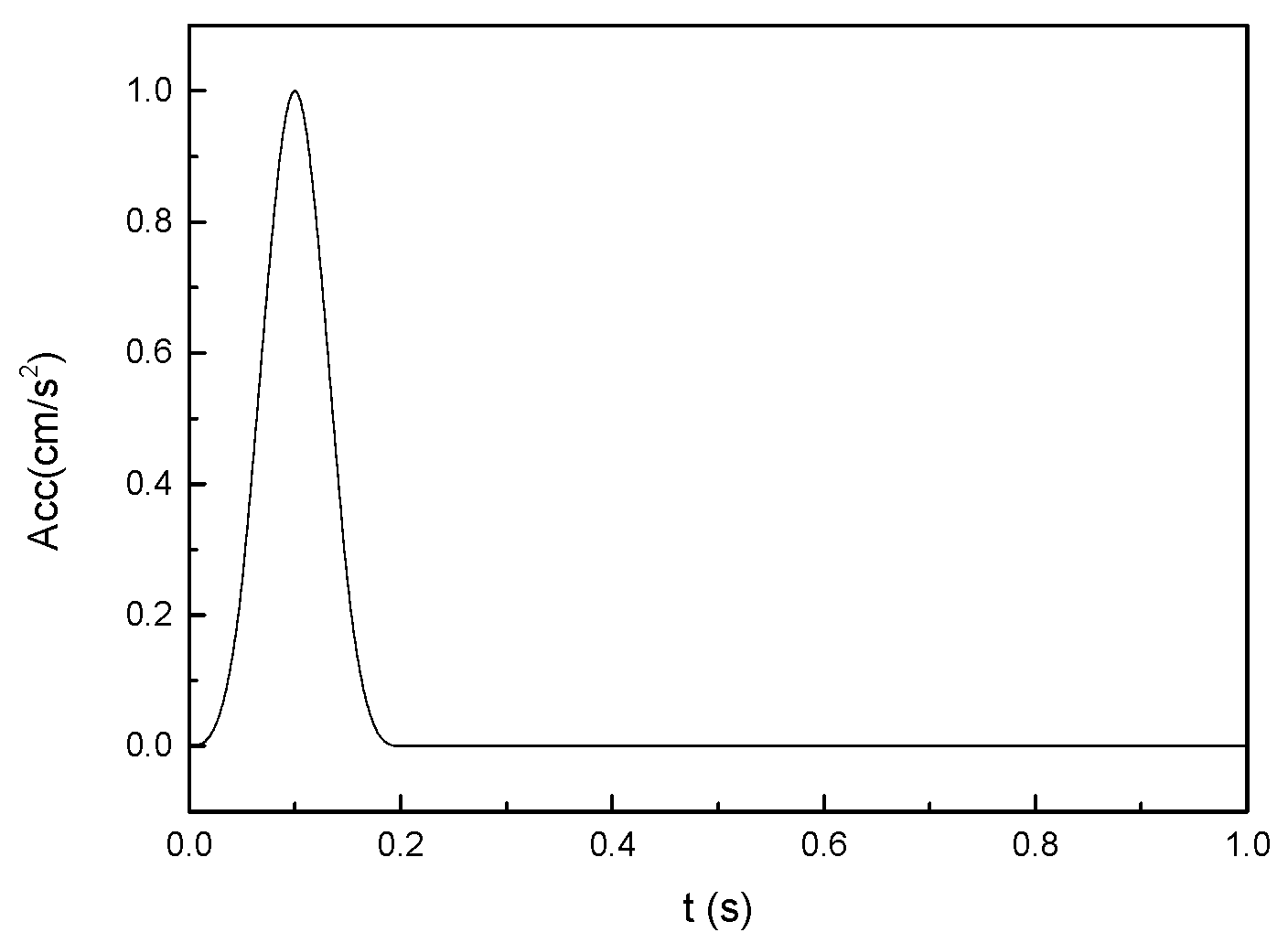
Based on the wave propagation theory, the response of each point on the surface of the basin at the bottom vertical incidence was calculated using the explicit solver of ABAQUS. The unit pulse width in this paper is 0.2, as shown in Figure 9. The acceleration time course is shown in Equation (13). The main distribution of the spectrum of this course covers most of the frequency domain of interest in engineering.

$$a\left(t\right)=\left\{\begin{array}{c}16\times {\left(\frac{t}{0.2}\right)}^3; 0<t\le 0.05\\ 1-48\times \left(\frac{t}{0.2}\right)\times {\left(\frac{t}{0.2}-0.5\right)}^2; 0.05<t\le 0.1\\ 1+48\times \left(\frac{t}{0.2}-1\right)\times {\left(\frac{t}{0.2}-0.5\right)}^2; 0.1<t\le 0.15\\ -16\times {\left(\frac{t}{0.2}-1\right)}^3; 0.15<t\le 0.2\\ 0; t>0.2\end{array}\right.$$

(13)

Figure 9. Time history of seismic input.

3.2. Validation of the Numerical Model

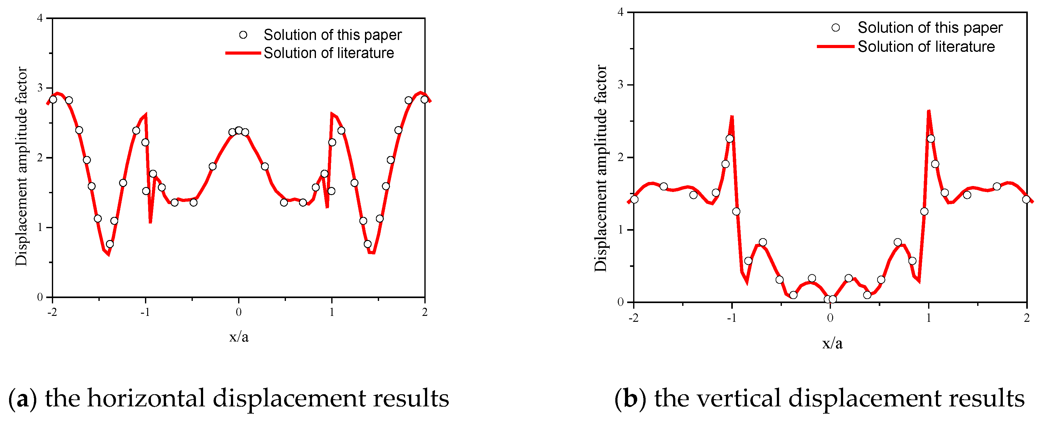
In order to verify the accuracy of the 2D site response simulated in this paper, the semicircular concave valley model from the literature was selected as the research object for simulation verification. The horizontal and vertical linear elastic displacement responses of the ground surface under the vertical incidence of plane P-SV waves were calculated and compared with the literature results. The relevant calculation parameters with dimensionless frequencies were as follows:

$$\eta =\frac{2a}{{\lambda }_s}=2$$

(14)

where $a$ is the radius of a semicircle and λs is the shear wave length of a half-space medium. The uniform half-space elastic medium has a density of ρ = 1800 kg/m³, a Poisson’s ratio υ = 1/3, and a shear wave velocity $V_s$ = 400 m/s. The size of the semi-circular concave valley was taken as 800 × 300, and the valley radius $a$ = 100 m.

As can be seen from the comparison results of the surface displacement amplitudes in Figure 10, the calculated results in this paper were basically consistent with those in the literature [31], indicating that the artificial boundary adopted in this paper could smoothly absorb the external scattering propagation to avoid reflection errors, and the corresponding ground motion input was successfully realized.

Figure 10. Accuracy validation of the FEM.

3.3. Extraction Methods and Parameter Definitions

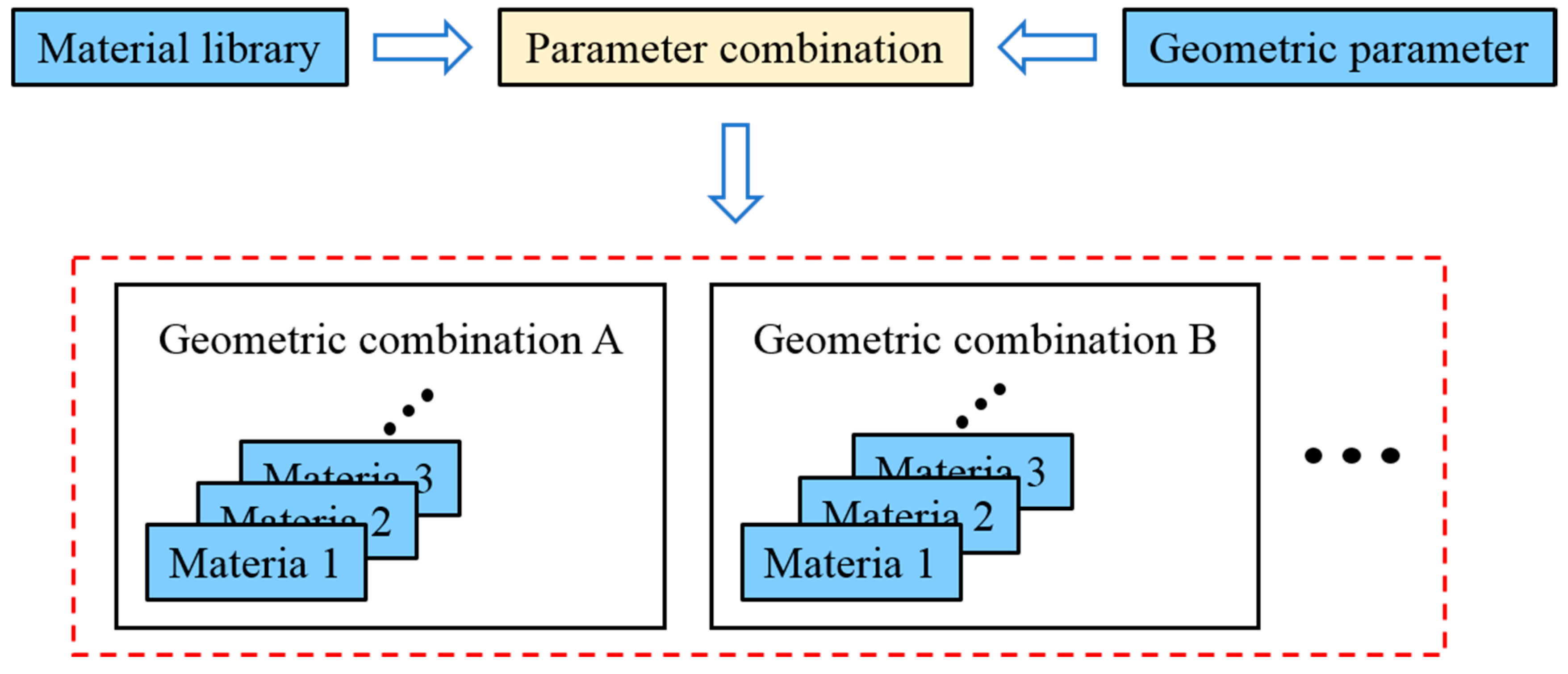
In order to expand the samples, the manual modeling of the ABAQUS interactive interface was abandoned and Python programming was used to implement parametric modeling. As shown in Figure 11, by setting reasonable ranges of geometric and media properties, different combinations were traversed to generate basin models with different site conditions to build the sample database.

Figure 11. Sample expansion process.

The specific implementation steps were as follows:

(1)

A material library was constructed for the selection of basin media diversity;

(2)

Python script was used to automatically modify basin geometry parameters such as soil depth, shape ratio, and dip angle to combine a large number of models;

(3)

Each material was combined by different geometry combinations in the material library to generate input files for subsequent calculations;

(4)

The basin model was submitted in batches to a supercomputer platform for calculation using Python scripts and the results were extracted to establish a database.

In this paper, the basin amplification factor was defined as the ratio of the peak acceleration of the surface to the peak acceleration of the incident wave, as shown in Equation (15):

$${\alpha }_p=\left|\frac{a_{\max ,surface}}{a_{\max ,input}}\right|$$

(15)

Since the maximum amplitude of the input pulse in this paper was 1, the amplification factor was equal to the peak value of the ground acceleration.

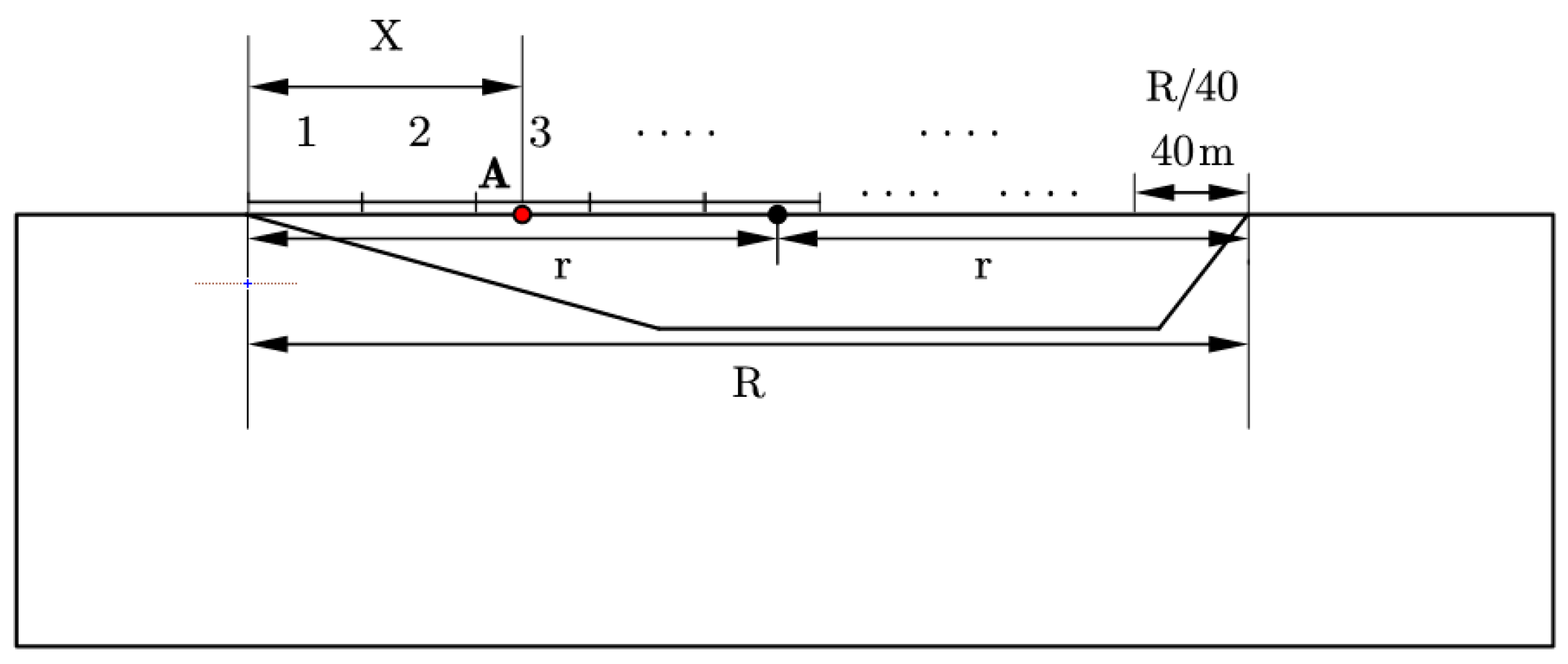
In this paper, the width of the basin was divided into several areas of equal length of 40 m [32], with the center of the basin as the origin and the half-width as the positive and negative half-axis, as shown in Figure 12.

Figure 12. Hazard location diagram.

The coordinates of the hazard location, expressed as the distance from the center of the basin, were obtained by Equation (16) below:

$$Y=\left[\frac{X}{40}\right]-\left[\frac{R}{80}\right]$$

(16)

$X$ was the distance from the left edge of the basin, $R$ was the width of the basin, and the values in parentheses are rounded.

Considering the symmetry of the basin, there were two hazard locations symmetrically distributed on both sides of the basin, this paper used a vector to characterize the area where the hazard location was located. The specific vector form is shown in Table 2, which contained three elements. The element positions represented the small dip side distribution, the symmetric distribution, and the large dip side distribution, where the position in the vector of the element with the largest absolute value represented the area where the hazard location was located, and the specific value represented the distance of the point from the center of the basin.

Table 2. Three vectors representing the hazard location.

Amplification Region	$\mathbf{Label} \left(\overrightarrow{\mathit{L}}\right)$
Asymmetric left side	$[\left|Y\right|, 0, 0]$
Symmetries	$[0, \left|Y\right|, 0]$
Asymmetric right side	$[0, 0, \left|Y\right|]$

For the final results, Python code was also written in this paper to extract the basin surface acceleration time history in batches.

4. Basin Amplification Models Based on CNN

4.1. Training Samples and Models

According to Section 2.2, the original sample data were obtained by numerically simulating the dynamic response of 756 basin models. After a reasonable analysis of the influence of each parameter on the basin amplification characteristics, it was finally determined that the input parameters of the basin amplification characteristics prediction model were the shape ratio (S), depth (H), small dip angle (θ₁) and big dip angle (θ₂), wave velocity ratio (C), damping coefficient α, damping coefficient β, and fundamental frequency of the site. A CNN was used to build the prediction model of the basin amplification characteristics. Three types of prediction models were established as shown in Table 3. The first two models predict the peak value of the amplification factor and the hazard location, respectively. The third model predicted both the amplification factor and the hazard location.

Table 3. Input and output parameters of prediction models.

Model	Input Layer Parameter	Output Layer Parameter
CNN factor prediction (CNN-AF)	S, H, θ1, θ2, C, α, β, f	Amplification (${\displaystyle {\alpha }_P}$)
CNN location prediction (CNN-RL)	S, H, θ1, θ2, C, α, β, f	Location (L)
CNN amplification parameters prediction (CNN-AP)	S, H, θ1, θ2, C, α, β, f	Amplification (${\alpha }_P$)and Location (L)

Based on the established basin database, the designed CNN was trained and tested. As shown in Table 4, there were 756 basin samples in the database, which were randomly divided into the training data set, testing data set, and validation data set according to a certain proportion.

Table 4. The division of samples.

	Basin Sample	Training Data Set	Validation Data Set	Testing Data Set
Number	756	605	120	151

4.2. Optimization of CNN Models

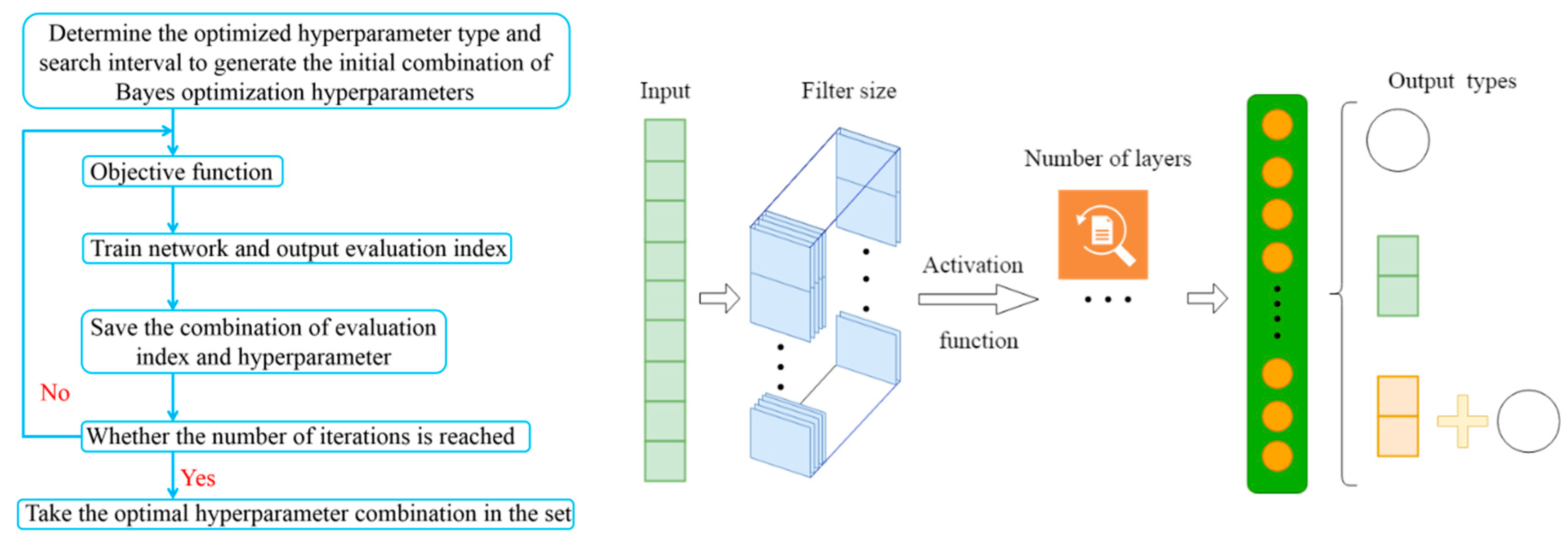
The network structure used in this paper followed MatConvNet (a MATLAB toolbox implementing CNNs for computer vision applications). In the CNN prediction model built in this paper, the input data were in 1D format, the pooling process was eliminated, and the filling operation was added to avoid feature loss. The parameters of the neural network can be divided into model parameters and model hyper-parameters. The model parameters can be automatically adjusted during neural network training according to certain algorithms without human intervention. The hyper-parameters cannot be estimated from the data, but can only be determined manually. The hyper-parameters of CNN generally include the number of convolutional layers, training frequency, learning rate, iteration frequency, etc. The structure and hyper-parameters of CNN generally need to be set in advance and then continuously optimized. The Bayesian optimization method of MATLAB was used to select the optimal model training using the root mean square error (RMSE) as the evaluation index, avoiding the complexity of manual parameter adjustment. The process of parameter fitting and optimizing was shown in Figure 13.

Figure 13. CNN model structure optimization process.

4.3. Performance Indicators

In order to better evaluate the effectiveness of the trained CNN model, the mean absolute error (MAE), root mean square error (RMSE), and the determinant factor (R²) were used as accuracy metrics; see Equations (17)–(19).

$$MAE=\frac{1}{n}{\displaystyle \sum _{i=1}^n\left|y_i^{}-f(x_i)\right|}$$

(17)

$$RMSE=\sqrt{{{\displaystyle \sum _{i=1}^n\frac{1}{n}\left(f(x_i)-y_i^{}\right)}}^2}$$

(18)

$$R^2=1-\frac{{\displaystyle \sum {(y_i-f(x_i))}^2}}{{\displaystyle \sum {(y_i-\overline{y})}^2}}$$

(19)

The combined use of MAE, RMSE, and R² provides a more comprehensive evaluation of the results. MAE and RMSE focus on the accuracy of the predictions, while R² focuses on the explanatory power of the predictive model. Therefore, when assessing the predictive performance of a model, these three metrics are usually considered together to obtain clearer, more comprehensive, and more reliable evaluation results. The smaller the values of MAE and RMSE, the better the prediction accuracy of the CNN model. The range of the decision factor (R²) was in the range [0~1], and its value closer to 1 indicated a better fitting effect.

5. Basin Amplification Characteristics Prediction

5.1. Results of Bayesian Optimization

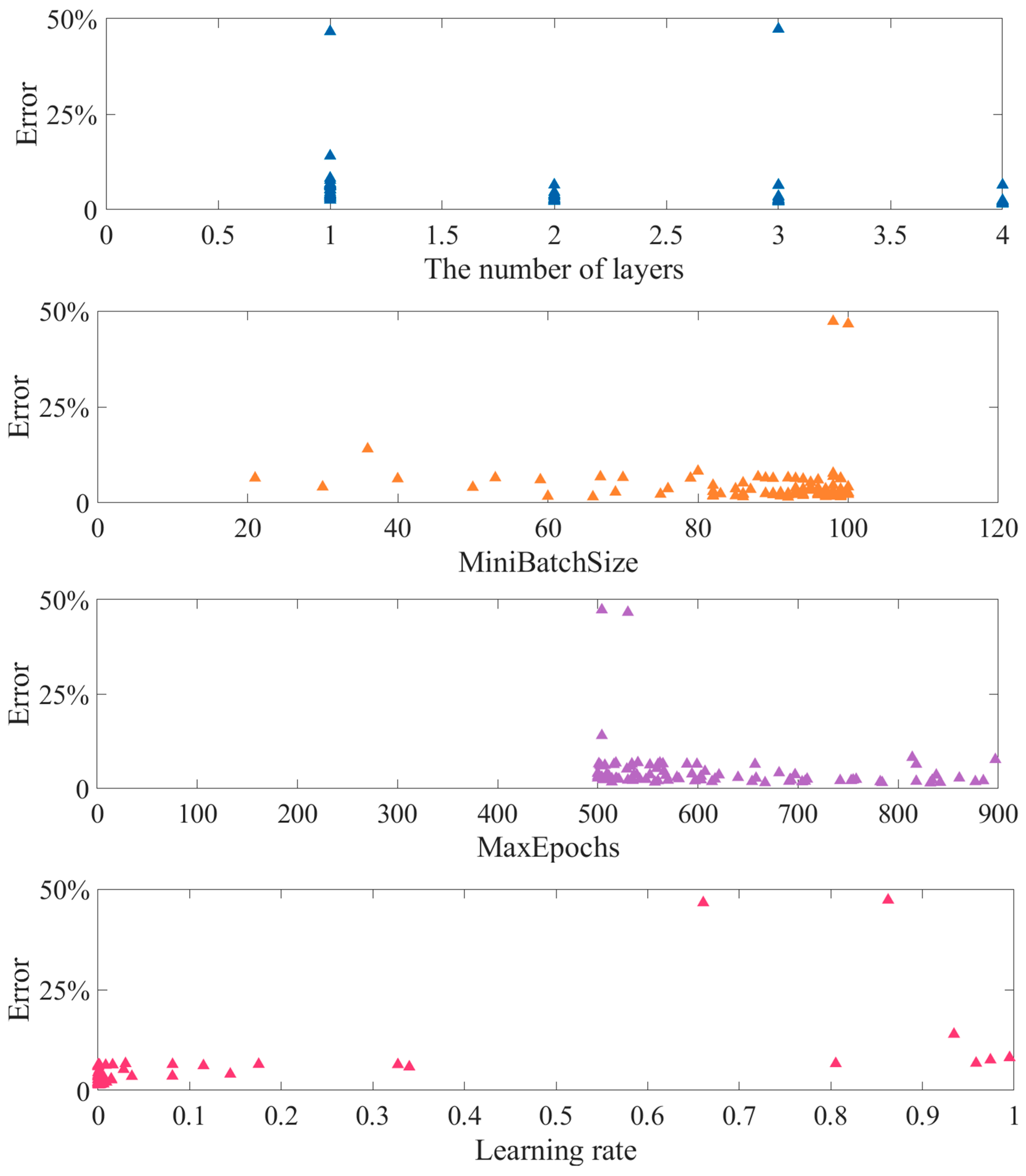
Taking the CNN-AF model as an example, the data set was input into the model, the Bayesian optimizer was used to select the hyper-parameters, and the optimization results for each hyper-parameter are shown in Figure 14. We further analyzed the influence of network parameters on the results. The results show the following: (1) There were large errors when the values of the MaxEpochs were set too low. Increasing the number of training epochs could avoid adverse events. (2) The MiniBatchSize was not appropriate to take too large values. In this case, the MiniBatchSize of 40–95 could ensure an ideal effect. (3) It is recommended to set a low learning rate. When the value was low, the achieved error was small and close to 0. (4) A deeper network layer could obtain a smaller prediction error. With the parameterization analysis, the best design scheme (network structure and hyper-parameters) of the CNN can be determined through Bayesian optimization. By synthesizing the optimization results of each hyper-parameter (as shown in Figure 14), when the number of convolutional layers was 4, the MiniBatchSize was 92, the MaxEpochs was 832, and the learning rate was 0.0073, the error of the model was minimal. The detailed network structure is shown in Table 5.

Figure 14. Hyper-parameters optimization results of CNN-AF model.

Table 5. Structural parameters of the CNN.

	Type	C1	C2	C3	C4
Kernel number	CNN-AF	95	190	380	-
	CNN-RL	127	254	508	1016
	CNN-AP-8	128	256	512	1024
Kernel size	CNN-AF	[3,1]	[3,1]	[3,1]	-
	CNN-RL	[3,1]	[4,1]	[4,1]	[4,1]
	CNN-AP-8	[5,1]	[5,1]	[5,1]	[5,1]
Stride	CNN-AF	1	1	1	-
	CNN-RL	1	1	1	1
	CNN-AP-8	1	1	1	1
Padding	CNN-AF	0	0	0	-
	CNN-RL	0	0	0	0
	CNN-AP-8	0	0	0	0
Activation	CNN-AF	LeakyReLU	LeakyReLU	LeakyReLU	-
	CNN-RL	LeakyReLU	LeakyReLU	LeakyReLU	LeakyReLU
	CNN-AP-8	LeakyReLU	LeakyReLU	LeakyReLU	LeakyReLU

Using the same optimization method, the hyper-parameter optimization results of the three models CNN-RL and CNN-AP-8 could also be obtained. The network structure and parameters of the optimal model were shown in Table 5.

5.2. Results of Each Prediction Model

5.2.1. Prediction of Peak Amplification Factor

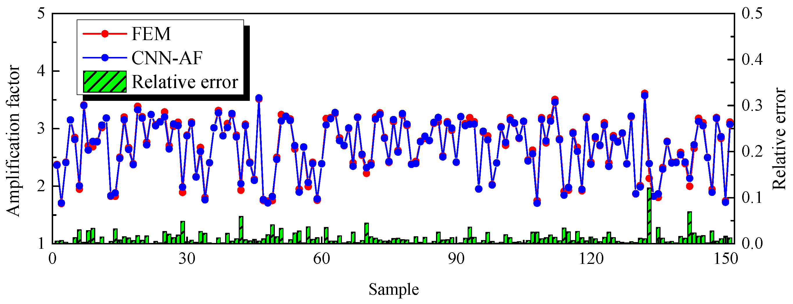
The CNN-AF amplification factor peak prediction model was trained and validated using the basin sample database described in Section 3. Based on 151 test samples, the error between the predicted value of the CNN-AF model and the simulated value of the FEM is shown in Figure 15. The mean values obtained from three training sessions were used to characterize the stable network, and the evaluation indicators of the CNN-AF model are shown in Table 6. The obtained mean RMSE of the training set was 3.4% and that of the test set was 5.1%.

Figure 15. Accuracy of CNN-AF model in predicting amplification factor.

Table 6. The evaluation indicators of CNN-AF model.

Name	MAE (Train/Test)	RMSE (Train/Test)	R2 (Train/Test)
CNN-AF	0.027/0.0385	0.0344/0.0509	0.9998/0.9995

5.2.2. Prediction of Hazard Location

The CNN-RL hazard location prediction model was also trained three times to obtain a stable prediction model. The prediction accuracy refers to the probability that the prediction area is symmetrical amplification, small inclination amplification or large inclination amplification. It can be seen from Table 7 that the mean prediction value of the amplification region was 94.70%. The average RMSE of the specific location in the correctly predicted area was about 2, as the width of the basin was divided into several areas of equal length of 40 m in this paper, which means that the error between the predicted and true specific location was about 80 m.

Table 7. The evaluation indicators of CNN-RL model.

CNN-RL	Direction	MAE	RMSE	R2
1	0.9338	1.2025	1.8211	0.9534
2	0.9669	1.3593	2.1358	0.9534
3	0.9404	1.3725	2.1660	0.9437
Average value	0.9470	1.3114	2.0410	0.9502

5.2.3. Joint Prediction Model for Basin Amplification Characteristics

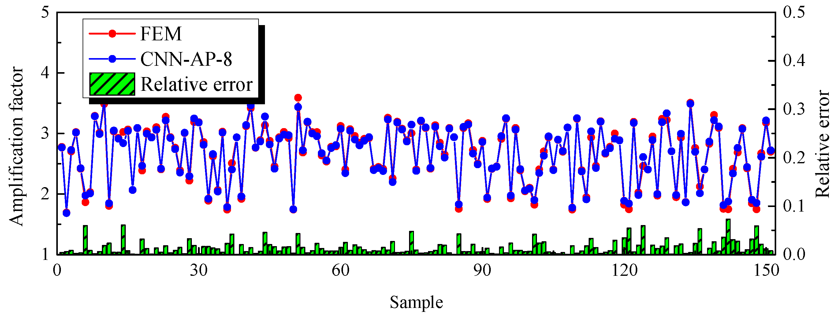
The prediction models in the previous two sections show that CNN can be used for either single or multiple outputs. In this section, the peak value of the amplification factor, which reflects the basin amplification characteristics, was combined with the hazard locations as the outputs of the prediction model. The eight parameters of the CNN-AF were used as the input of the CNN-AP-8, and the model output was based on the CNN-AF amplification factor peak output while considering the value of the hazard location. Figure 16 shows the relative error of the CNN-AP-8 model in predicting the amplification factor, which was below 10 percent for all 151 samples tested, and the evaluation indicators are shown in Table 8.

Figure 16. Accuracy of CNN-AP-8 model in predicting amplification factor.

Table 8. The evaluation indicators of CNN-AP-8 model.

CNN-AP-8	Direction	MAE (AF/RL)	RMSE (AF/RL)	R2 (AF/RL)
1	0.9139	0.0381/1.1123	0.0519/1.709	0.9881/0.9683
2	0.9470	0.0478/1.4589	0.0624/2.2816	0.9822/0.9264
3	0.9139	0.0403/1.0615	0.0581/1.7479	0.9857/0.9668
Average value	0.9249	0.0421/1.2109	0.0575/1.9128	0.9853/0.9538

As shown in Table 9, the accuracy of the CNN-AP-8 model was lower than that of the CNN-AF model, but the errors were all around 1%. Compared with CNN-RL, the CNN-AP-8 joint model was only slightly lower than CNN-RL in direction prediction accuracy, by 2.2%, and was better than CNN-RL in other evaluation indicators.

Table 9. Comparison of CNN-AP-8 model with CNN-RL and CNN-AF models.

Name	Direction	MAE	RMSE	R2
CNN-AF	\	0.0385	0.0509	0.9995
CNN-RL	0.9470	1.3114	2.0410	0.9502
CNN-AP-8	0.9249	0.0421/1.2109	0.0575/1.9128	0.9853/0.9538

In summary, the joint prediction model was only about 1% lower than the dedicated CNN-AF in predicting the amplification factor. However, the overall prediction effect of the hazard location was better than the corresponding special model CNN-RL, and there was only a disadvantage in the direction prediction. This may be because the output of the joint prediction model has one more amplification factor peak, which increases the complexity of the model. Therefore, the CNN-AP-8 model was finally selected for the prediction of basin amplification characteristics in this paper.

5.3. Optimize Input Parameters to Build Prediction Models

The input parameters of the final prediction model CNN-AP-8 in this paper include S, C, H, θ₁, θ₂, α, β, and f. The following is a sensitivity analysis of the shape ratio, the dip angle parameter, which characterizes the geometric characteristics, and the wave velocity ratio parameter which characterizes the medium characteristics.

5.3.1. Effect of Shape Ratio

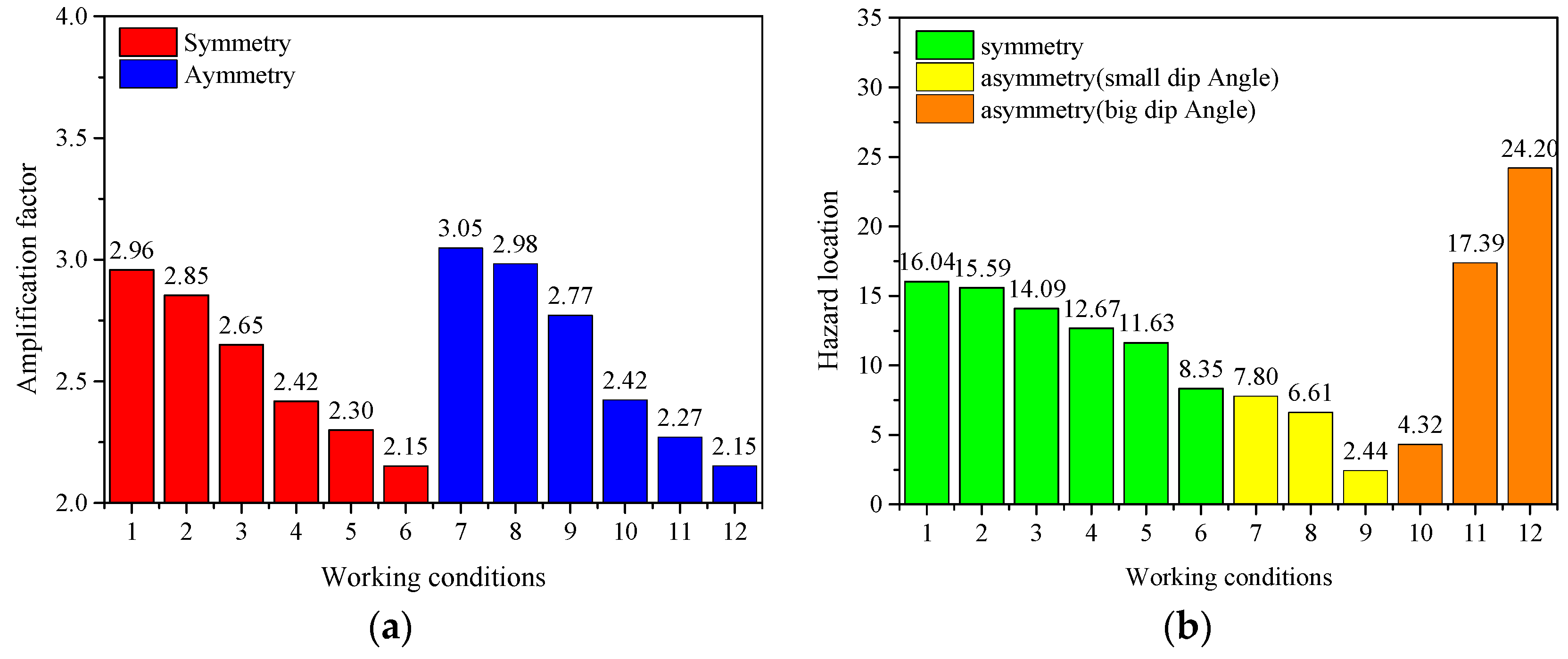
Eight conditions were set to observe the change in the predicted results of the amplification factor and the hazard location. Only the shape ratio parameter was modified and other parameters were kept constant. The shape ratio of working conditions 1–4 is 0.15, 0.2, 0.3, and 0.4, and the same working condition ratio is adopted for working conditions 5–8. The sensitivity analysis of the shape ratio is performed in both symmetric and asymmetric cases.

From the predicted results of the amplification factor, Figure 17, it can be seen that the amplification factor increases with the increase in the shape ratio factor for both symmetric and asymmetric basins. The predicted amplification factor of asymmetric basins shows that the amplification factor was higher than that of symmetric basins under the same shape ratio. On the contrary, in the hazard location prediction, the hazard location is closer to the center of the basin with the increase in the shape ratio. The analysis of the above results may be due to the narrower basin with a larger shape ratio which results in a more pronounced basin focus effect. The hazard location of the asymmetric basin is closer to the center of the basin than the symmetric basin under the same shape ratio.

Figure 17. Max value of amplification factor and hazard location from different shapes. (a) Amplification factor. (b) Hazard location.

5.3.2. Effect of Wave Velocity Ratio

As in the previous section, only the wave speed ratio is modified for the sensitivity analysis. The wave speed ratio of working conditions 1–6 is 2.5, 3, 4, 5, 6, and 7.5, and the same wave speed ratio is adopted for working conditions 7–12. From Figure 18, it can be seen that as the wave speed ratio increases, the shear wave speed decreases and the amplification factor of both symmetrical and asymmetrical basins decreases accordingly. Similarly, the hazard location in the symmetric basin was also closer to the central location of the basin as the wave velocity ratio increased. The reason for this may be that the shear wave velocity was small, the seismic waves were lost more slowly in the repeated refraction of the soil layer to be focused in the central part of the basin and finally consumed by the damping of the soil. The asymmetric case was the opposite, being farthest from the center of the basin when the wave velocity ratio was minimal, which may be an effect of the dip angles on both sides of the basin.

Figure 18. Max value of amplification factor and hazard location from different shear wave velocities. (a) Amplification factor. (b) Hazard location.

5.3.3. Effect of Dip Angle

The significant difference in hazard location between symmetrical and asymmetrical configurations in the first two sections reflects the effect of the inclination angle. In this section, we only modify the inclination angle to perform sensitivity analysis, and each working condition is presented in Table 10. Regarding the amplification factor, as shown in Figure 19a, the effect of the inclination angle is not obvious, and there is only a positive correlation within a certain range. In the case of asymmetry, through the analysis of working conditions 2 and 7, as well as working conditions 5 and 8, it is apparent that the amplification factor is closer to the symmetrical case of a large dip angle. In terms of hazard location prediction, as shown in Figure 19b, when the dip angle is less than 80°, the hazard location is closer to the center of the basin as the dip angle increases. Similarly, in the case of asymmetry, by analyzing working conditions 2 and 7, as well as working conditions 5 and 8, we can see that the hazard location, in this case, is closer to that in the case of symmetry of a large dip angle.

Table 10. Different angles parameters of basin.

No.	S	C	H/m	θ1/°	θ2/°	α	β	f/Hz
1	0.2	2.5	300	15	15	0.044	0.00088	0.5
2	0.2	2.5	300	20	20	0.044	0.00088	0.5
3	0.2	2.5	300	30	30	0.044	0.00088	0.5
4	0.2	2.5	300	45	45	0.044	0.00088	0.5
5	0.2	2.5	300	60	60	0.044	0.00088	0.5
6	0.2	2.5	300	80	80	0.044	0.00088	0.5
7	0.2	2.5	300	20	30	0.044	0.00088	0.5
8	0.2	2.5	300	20	60	0.044	0.00088	0.5

Figure 19. Max value of amplification factor and hazard location from different angles. (a) Amplification factor. (b) Hazard location.

The analysis in the above subsections shows that the geometric and media factors considered in this paper have important effects on the peak surface amplification coefficients of the basin, which were necessary parameters for predicting the amplification characteristics of the basin and validating their reasonableness as input parameters of the neural network.

5.3.4. Comparison of Results of Prediction Models with Different Input Parameters

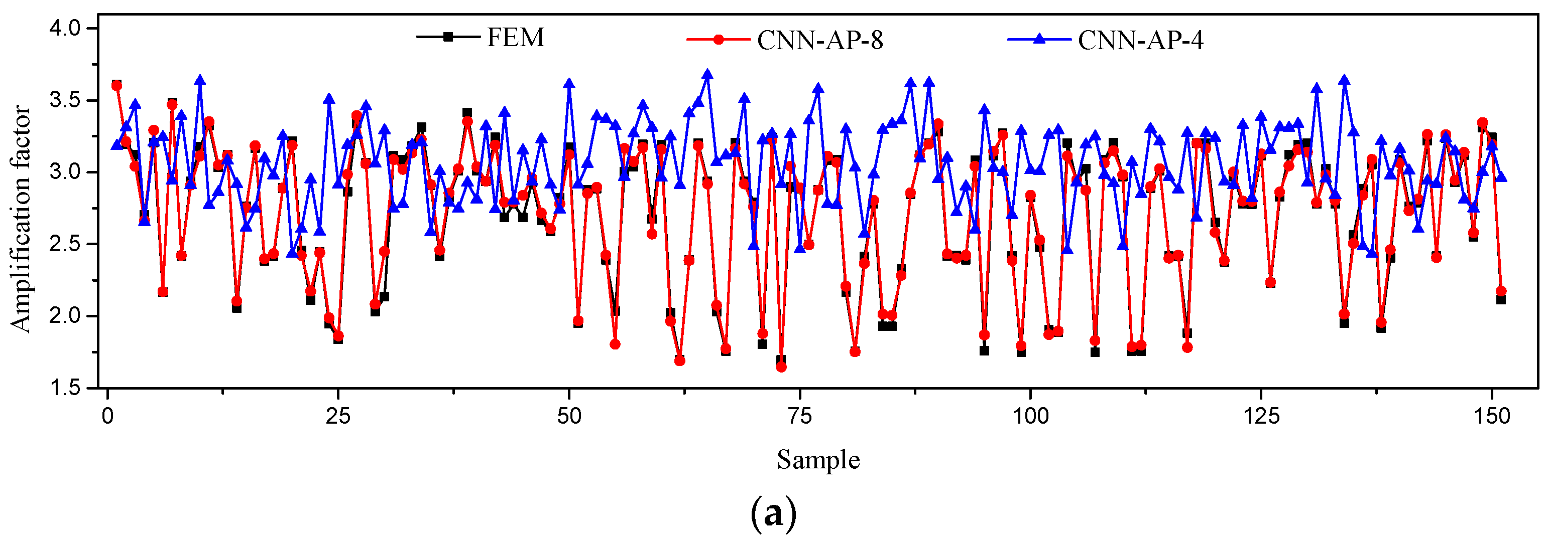
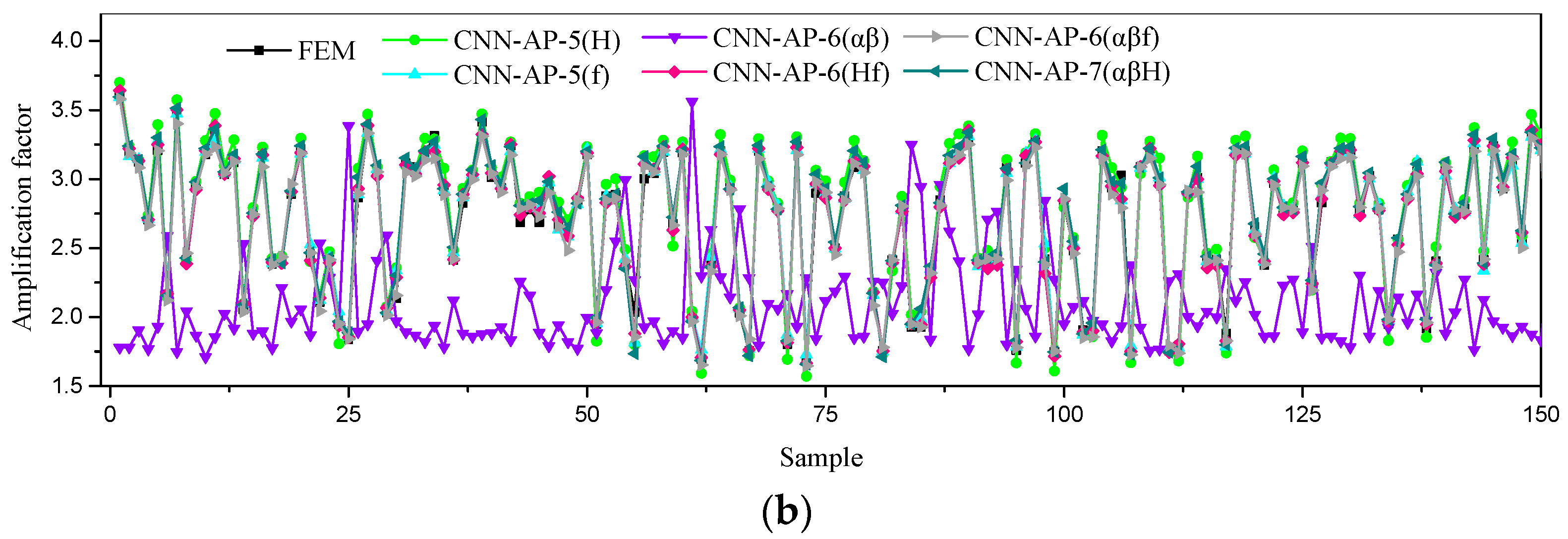
Based on the four factors S, C, θ₁, and θ₂, the CNN-AP-4 prediction model was first established. As shown in Figure 20a, we found that the recognition ability of the neural network was poor due to the limited input parameters. On this basis, the relative importance of H, f, and damping coefficients α and β were studied, respectively. As shown in Table 11, six prediction models, CNN-AP-5 (H), CNN-AP-5 (f), CNN-AP-6 (αβ), CNN-AP-6 (Hf), CNN-AP-7 (αβH), and CNN-AP-7 (αβf), were established to discuss and analyze the influence of each factor on the prediction model. The prediction results of each model for the amplification factor are shown in Figure 20b and Table 12, and the prediction results of the hazard location are shown in Table 13.

Figure 20. The results of amplification factor predicted by different models. (a) Comparison of prediction results between CNN-AP-4 and CNN-AP-8. (b) Comparison of prediction results of prediction models with different input parameters.

Table 11. Input and output parameters of prediction models.

Model	Input Layer Parameter	Output Layer Parameter
CNN-AP-5 (H)	S, C, θ1, θ2, H	${\alpha }_P$ and L
CNN-AP-5 (f)	S, C, θ1, θ2, f
CNN-AP-6 (αβ)	S, C, θ1, θ2, α, β
CNN-AP-6 (Hf)	S, C, θ1, θ2, H, f
CNN-AP-7 (αβH)	S, C, θ1, θ2, α, β, H
CNN-AP-7 (αβf)	S, C, θ1, θ2, α, β, f

Table 12. Comparison of evaluation indicators between CNN-AP-8 model and different prediction models on amplification factor.

Name	MAE	RMSE	R2
CNN-AP-8	0.0421	0.0575	0.9853
CNN-AP-4	0.5338	0.6892	−1.0192
CNN-AP-5 (H)	0.0798	0.0946	0.9619
CNN-AP-5 (f)	0.0327	0.0469	0.9906
CNN-AP-6 (αβ)	0.8390	0.9434	−2.7837
CNN-AP-6 (Hf)	0.0318	0.0428	0.9922
CNN-AP-7 (αβH)	0.0415	0.0584	0.9855
CNN-AP-7 (αβf)	0.0352	0.0491	0.9897

Table 13. Comparison of evaluation indicators between CNN-AP-8 model and different prediction models on hazard location.

Name	Direction	MAE	RMSE	R2
CNN-AP-8	0.9249	1.2109	1.9128	0.9538
CNN-AP-4	0.4040	10.5675	11.8515	−0.5094
CNN-AP-5 (H)	0.9470	1.0091	2.6531	0.9544
CNN-AP-5 (f)	0.9669	0.9729	1.6513	0.9661
CNN-AP-6 (αβ)	0.3841	10.2799	12.4476	−0.5890
CNN-AP-6 (Hf)	0.9735	1.0291	1.6377	0.9758
CNN-AP-7 (αβH)	0.9669	1.3036	1.8822	0.9481
CNN-AP-7 (αβf)	0.9735	1.6464	1.9354	0.9598

It can be seen from the results that CNN-AP-6 (Hf) is the best in terms of amplification coefficient prediction, followed by CNN-AP-5 (f), whose indexes are better than CNN-AP-8. CNN-AP-6 (Hf) is the best in the prediction of hazard location, followed by CNN-AP-5 (f), whose indexes are better than CNN-AP-8. In addition, CNN-AP-4 and CNN-AP-6 (αβ) are worse than CNN-AP-8 in terms of amplification factor and hazard location prediction. A negative R² indicates that the performance of the regression model is worse than the average. By comparing the CNN-AP-4, CNN-AP-5 (f), and CNN-AP-5 (H) models, it can be found that, based on the CNN-AP-4 model, the accuracy of predicting amplification factor and hazard location has been greatly improved after adding fundamental frequency or soil thickness parameters. Meanwhile, the same rule can be found by comparing CNN-AP-6 (αβ), CNN-AP-7 (αβH), and CNN-AP-7 (αβf) models.

6. Conclusions

In this paper, an artificial intelligence method of CNN was used to predict the amplification characteristics of the standard basin, focusing on the influence of the geometrical and soil mechanical parameters of the basin on the surface amplification in the case of a distant earthquake ignoring the effects of the source and the propagation path. The parametric modeling of the finite element software ABAQUS was implemented to build a batch model of the basin. According to the amplification characteristics of the basin, the special neural networks for peak amplification coefficients and hazard locations, as well as a joint prediction network for both, were established, respectively. The three types of networks were trained to use the influencing factors of the basin amplification characteristics as the input of CNN to predict the surface amplification characteristics of standard basins and combined with Bayesian optimization methods to select the best network parameters to improve the accuracy of the network. Finally, the sensitivity of specific geometric and media parameters to the effect of surface amplification was analyzed based on the final selected eight-parameter joint prediction model CNN-AP-8 predictions. The results of the computational analysis show that:

(1)

In predicting the location of amplification hazards, labels were assigned using vectors. The basin was divided into three categories: symmetric, small dip asymmetry, and big dip asymmetry. The prediction accuracy of the hazard location reached 94.70%, and the mean square error for predicting specific locations was about 2, as the width of the basin was divided into several areas of equal length of 40 m in this paper, which means that the error between the predicted and true specific location was about 80 m.

(2)

Comparing the eight-parameter CNN-AP-8 prediction model against two dedicated prediction models for amplification characteristics demonstrated that the joint prediction model could predict basin amplification characteristics comprehensively, and the accuracy was basically the same as that of two dedicated prediction models.

(3)

In the parameter sensitivity analysis, by comparing the accuracy of the model under different input parameters, it was found that the shape ratio, wave velocity ratio, dip angle, soil thickness, and fundamental frequency were very important input factors. The prediction model based on these factors has improved the accuracy of the amplification factor and the hazard location. The prediction accuracy of the hazard location was up to 97.35%, and the mean square error for predicting specific locations was about 1. The true error in the 40 m segmented basins model was about 40 m.

(4)

The basin models in this paper were all single-layer standard simplified models, which were still different from the actual basins. The soil stratification can be further considered in the future. At the same time, the incident wave also has an important effect on surface amplification. After further considering the effects of the incident wave frequency, incident angle, and other factors, and whether the CNN can have a better prediction effect needs further study.

(5)

Compared with the establishment of complex numerical models and relying on a high level of computational conditions, the prediction method in this paper can quickly predict the peak amplification and the hazard location, only through the input of a few simple geometrical and physical parameters, and it has a better prospect of engineering applications.

However, further research is needed to study the predictive modeling of complex local sedimentary basins:

(1)

The 2D-SH and 2D-P_SV models are two basic problems in 2D. Due to the limitation of the analysis process of ABAQUS software, it is difficult to simulate the SH problem based on ABAQUS, so we used the P-SV model. In future research, we will predict the features of the SH problem.

(2)

Predictive modeling of complex local sedimentary basins based on other machine learning methods (e.g., tree models, etc.) and complex network frameworks. The SHAP (Shapley Additive Explanations) method can be applied to the machine learning model to explain how much each sample or each feature contributes to the corresponding predicted value when performing sensitivity analyses on the parameters.

(3)

The presence of a building at a specific location at the top of the soft soil layer will definitely alter the time history of the seismic motion experienced at that point, compared to the motion that would have occurred if the building was not present. The effect of the superstructure on surface magnification is not considered in this study. Therefore, subsequent studies could include consideration of various factors associated with buildings experiencing seismic amplification movements.

(4)

The Abaqus2Matlab [33] application can be tried to automate the task by passing the ABAQUS results (i.e., training data) directly to the MatConvNet toolbox without the need to switch languages between Python and MATLAB.

References

- Bard, P.-Y.; Campillo, M.; Chavez-Garcia, F.; Sanchez-Sesma, F. The Mexico earthquake of September 19, 1985—A theoretical investigation of large-and small-scale amplification effects in the Mexico City Valley. Earthq. Spectra 1988, 4, 609–633. [Google Scholar] [CrossRef]
- Fletcher, J.B.; Wen, K.-L. Strong ground motion in the Taipei basin from the 1999 Chi-Chi, Taiwan, earthquake. Bull. Seismol. Soc. Am. 2005, 95, 1428–1446. [Google Scholar] [CrossRef]
- Jagota, V.; Sethi, A.P.S.; Kumar, K. Finite element method: An overview. Walailak J. Sci. Technol. (WJST) 2013, 10, 1–8. [Google Scholar]
- Semblat, J.-F.; Brioist, J. Efficiency of higher order finite elements for the analysis of seismic wave propagation. arXiv 2009, arXiv:0901.3715. [Google Scholar] [CrossRef]
- Gazetas, G.; Kallou, P.; Psarropoulos, P. Topography and soil effects in the Ms 5.9 Parnitha (Athens) earthquake: The case of Adámes. Nat. Hazards 2002, 27, 133–169. [Google Scholar] [CrossRef]
- Riga, E.; Makra, K.; Pitilakis, K. Investigation of the effects of sediments inhomogeneity and nonlinearity on aggravation factors for sedimentary basins. Soil Dyn. Earthq. Eng. 2018, 110, 284–299. [Google Scholar] [CrossRef]
- Bazyar, M.H.; Song, C. Analysis of transient wave scattering and its applications to site response analysis using the scaled boundary finite-element method. Soil Dyn. Earthq. Eng. 2017, 98, 191–205. [Google Scholar] [CrossRef]
- Meza-Fajardo, K.C.; Varone, C.; Lenti, L.; Martino, S.; Semblat, J.-F. Surface wave quantification in a highly heterogeneous alluvial basin: Case study of the Fosso di Vallerano valley, Rome, Italy. Soil Dyn. Earthq. Eng. 2019, 120, 292–300. [Google Scholar] [CrossRef]
- Moczo, P.; Kristek, J.; Bard, P.-Y.; Stripajová, S.; Hollender, F.; Chovanová, Z.; Kristeková, M.; Sicilia, D. Key structural parameters affecting earthquake ground motion in 2D and 3D sedimentary structures. Bull. Earthq. Eng. 2018, 16, 2421–2450. [Google Scholar] [CrossRef]
- Liang, J.; Liu, Z.; Huang, L.; Yang, G. The indirect boundary integral equation method for the broadband scattering of plane P, SV and Rayleigh waves by a hill topography. Eng. Anal. Bound. Elem. 2019, 98, 184–202. [Google Scholar] [CrossRef]
- Anquez, P.; Glinsky, N.; Cupillard, P.; Caumon, G. Impacts of geometric model simplifications on wave propagation—Application to ground motion simulation in the lower Var valley basin (France). Geophys. J. Int. 2022, 229, 110–137. [Google Scholar] [CrossRef]
- Makra, K.; Raptakis, D.; Chavez-Garcia, F.; Pitilakis, K. How important is the detailed knowledge of a 2D soil structure for site response evaluation. In Proceedings of the 12th European Conference on Earthquake Engineering, London, UK, 9–13 September 2002. [Google Scholar]
- Makra, K.; Chávez-García, F.J.; Raptakis, D.; Pitilakis, K. Parametric analysis of the seismic response of a 2D sedimentary valley: Implications for code implementations of complex site effects. Soil Dyn. Earthq. Eng. 2005, 25, 303–315. [Google Scholar] [CrossRef]
- Karimi Ghalehjough, B.; Mahinroosta, R. Peak ground acceleration prediction by fuzzy logic modeling for Iranian plateau. Acta Geophys. 2020, 68, 75–89. [Google Scholar] [CrossRef]
- Yu, Y.; Li, J.; Li, J.; Xia, Y.; Ding, Z.; Samali, B. Automated damage diagnosis of concrete jack arch beam using optimized deep stacked autoencoders and multi-sensor fusion. Dev. Built Environ. 2023, 14, 100128. [Google Scholar] [CrossRef]
- Yu, Y.; Liang, S.; Samali, B.; Nguyen, T.N.; Zhai, C.; Li, J.; Xie, X. Torsional capacity evaluation of RC beams using an improved bird swarm algorithm optimised 2D convolutional neural network. Eng. Struct. 2022, 273, 115066. [Google Scholar] [CrossRef]
- Kim, S.; Hwang, Y.; Seo, H.; Kim, B. Ground motion amplification models for Japan using machine learning techniques. Soil Dyn. Earthq. Eng. 2020, 132, 106095. [Google Scholar] [CrossRef]
- Mir, A.A.; Çelebi, F.V.; Alsolai, H.; Qureshi, S.A.; Rafique, M.; Alzahrani, J.S.; Mahgoub, H.; Hamza, M.A. Anomalies prediction in radon time series for earthquake likelihood using machine learning-based ensemble model. IEEE Access 2022, 10, 37984–37999. [Google Scholar] [CrossRef]
- Lysmer, J.; Kuhlemeyer, R.L. Finite dynamic model for infinite media. J. Eng. Mech. Div. 1969, 95, 859–877. [Google Scholar] [CrossRef]
- Wang, M.; Liu, B.; Foroosh, H. Look-up table unit activation function for deep convolutional neural networks. In Proceedings of the 2018 IEEE Winter Conference on Applications of Computer Vision (WACV), Lake Tahoe, NV, USA, 12–15 March 2018. [Google Scholar]
- Nair, V.; Hinton, G.E. Rectified linear units improve restricted boltzmann machines. In Proceedings of the 27th international conference on machine learning (ICML-10), Haifa, Israel, 21–24 June 2010. [Google Scholar]
- Krizhevsky, A.; Sutskever, I.; Hinton, G.E. Imagenet classification with deep convolutional neural networks. Adv. Neural Inf. Process. Syst. 2012, 25, 84–90. [Google Scholar] [CrossRef]
- Lulu, Z. Improved recommendation system based on social trust relation. Comput. Appl. Softw. 2014, 31, 31–35. [Google Scholar]
- Riga, E.; Makra, K.; Pitilakis, K. Aggravation factors for seismic response of sedimentary basins: A code-oriented parametric study. Soil Dyn. Earthq. Eng. 2016, 91, 116–132. [Google Scholar] [CrossRef]
- Gélis, C.; Bonilla, L.F. Influence of a sedimentary basin infilling description on the 2-DP–SV wave propagation using linear and non-linear constitutive models. Geophys. J. Int. 2014, 198, 1684–1700. [Google Scholar] [CrossRef]
- Gélis, C.; Bonilla, L.F. 2-DP–SV numerical study of soil–source interaction in a non-linear basin. Geophys. J. Int. 2012, 191, 1374–1390. [Google Scholar]
- Gelagoti, F.; Kourkoulis, R.; Anastasopoulos, I.; Tazoh, T.; Gazetas, G. Seismic wave propagation in a very soft alluvial valley: Sensitivity to ground-motion details and soil nonlinearity, and generation of a parasitic vertical component. Bull. Seismol. Soc. Am. 2010, 100, 3035–3054. [Google Scholar] [CrossRef]
- Khanbabazadeh, H.; Iyisan, R.; Ansal, A.; Zulfikar, C. Nonlinear dynamic behavior of the basins with 2D bedrock. Soil Dyn. Earthq. Eng. 2018, 107, 108–115. [Google Scholar] [CrossRef]
- Zhu, C.; Thambiratnam, D.; Gallage, C. Inherent characteristics of 2D alluvial formations subjected to in-plane motion. J. Earthq. Eng. 2019, 23, 1512–1530. [Google Scholar] [CrossRef]
- Wang, H.-F.; Lou, M.-L.; Zhang, R.-L. Selection of Rayleigh damping coefficients for seismic response analysis of soil layers. Int. J. Geol. Environ. Eng. 2017, 11, 158–163. [Google Scholar]
- Ba, Z.; Liang, J. Diffraction of plane SV waves around an alluvial valley in layered half-space. Dizhen Gongcheng Yu Gongcheng Zhendong (Earthq. Eng. Eng. Vib.) 2011, 31, 18–26. [Google Scholar]
- Shengyin, Q.; Qifang, L.; Ruizhi, W. Basin amplification effect of seismic ground motion based on seismic wave numerical simulation in two-dimensional model. Earthq. Eng. Eng. Vib. 2021, 41, 14. [Google Scholar]
- Papazafeiropoulos, G.; Muñiz-Calvente, M.; Martínez-Pañeda, E. Abaqus2Matlab: A suitable tool for finite element post-processing. Adv. Eng. Softw. 2017, 105, 9–16. [Google Scholar] [CrossRef]
Disclaimer/Publisher’s Note: The statements, opinions and data contained in all publications are solely those of the individual author(s) and contributor(s) and not of MDPI and/or the editor(s). MDPI and/or the editor(s) disclaim responsibility for any injury to people or property resulting from any ideas, methods, instructions or products referred to in the content. |
© 2023 by the authors. Licensee MDPI, Basel, Switzerland. This article is an open access article distributed under the terms and conditions of the Creative Commons Attribution (CC BY) license (https://creativecommons.org/licenses/by/4.0/).