Optimizing Parameters for an Electrical Car Employing Vehicle Dynamics Simulation Program

Abstract

At the Faculty of Engineering of the University of Debrecen we have dealt with the design and construction of electric prototype race cars for more than a decade. With a focus on more conscious design and racing we developed a vehicle dynamics simulation program, which can be used to generate the dynamics functions of the cars from their technical characteristics and data. In this publication, we deal with the optimization of the technical parameters of the above-mentioned cars for various competition tasks using our simulation program. This is a completely new field of application of the used optimization methods. This concept and idea can effectively help student teams all over the world to prepare for various domestic and international competitions. One of the applied methods is a graphic procedure, the other one is the widely used “adaptive simulated annealing” (ASA). After a brief description of the simulation program, the applied optimization methods and developed MATLAB codes for them are described. Finally, to demonstrate the effectiveness of the methods, we optimize the parameters of a prototype race car for different competition tasks and present the obtained results.

1. Introduction

The Faculty of Engineering of the University of Debrecen has a long experience in the designing, development, and construction of prototype race cars with alternative (mainly electric) drive [1,2]. In the last few years, student teams at our faculty have designed and constructed several race cars with electric or pneumatic drive and have taken part in, and achieved success in, domestic and international competitions. In 2014 and 2015 the prototype race car, which was developed by the student team of the Department of Mechanical Engineering, scored first and second place in the MVM Race organized by the Hungarian Electric Works Ltd. The team from our faculty has also took part in the “Shell ECO Marathon” competition—which was organized in London in 2016 and 2017—and successfully completed the competition. For the more conscious design of the prototype race cars, a simulation program [3] was developed in the MATLAB/Simulink (9.5, R2018b) environment. This program has a modular structure, thus the different structural units of the car (electric motor, powertrain, front and rear suspension, and vehicle body) are simulated in separate modules. The above program, which is described briefly in Section 3, is capable of calculating the vehicle dynamic functions of the car from its technical data. The above data can, in certain cases, be found in the technical description of the different machine parts of the car, but in most cases the data have to be determined experimentally [4,5,6,7,8,9,10]. Regarding electric motors, for the experimental determination of the input simulation data and characteristics [6,7,8,9,10], a complex measurement system was developed previously by the authors [11].

Optimum selection (adjustment) [12] of the vehicle’s technical data is very important in racing, since even with a fundamentally good vehicle construction, the best possible result can only be achieved if the values of the above data are chosen properly for the specific competition task. To be able to find the optimal values of technical data, different optimization procedures were developed for our vehicle dynamics simulation program [3].

These procedures, and particularly their applications for the above specific purpose (which are described in detail in this publication), are novel, and differ from usual engineering applications.

In Section 2, a detailed review of the different optimization methods including “simulated annealing” together with their applications are presented. In Section 3, a brief description of our simulation program [3] is given, while in Section 4, the basic concepts of optimization are summarized. In Section 4.1 optimization applying a graphical procedure is presented, while in Section 4.2 optimization using simulated annealing (SA) [13,14,15,16] is described and applied for the determination of the optimal values of the technical data of the race car [3] that was the winner of the MVM Race in 2014, for different competition tasks.

2. Literature Review

In the field of optimization, numerous methods have been developed and applied to various engineering problems [17,18,19,20,21,22,23,24,25,26,27]. Widely used optimization algorithms and techniques are fuzzy logic [28,29], adaptive neuro-fuzzy inference systems [30,31], the Taguchi method [32,33], the grey system theory [26,34,35], teaching–learning-based optimization [36,37], genetic algorithms [38], particle swarm optimization [39], tabu search [40], and simulated annealing [13,14,15,16].

There is extensive literature on the optimization of vehicles using the above-mentioned algorithms and procedures. In [41], a multi-objective optimization is introduced applying the particle swarm algorithm to optimize the drivetrain and control system of a plug-in hybrid vehicle. In [42], a multi-objective optimization is presented using a genetic algorithm to improve acceleration performance, fuel consumption, and to mitigate emission of a vehicle. In [43], a genetic algorithm is applied to optimize the drivetrain of an electric vehicle. In [44], an evolutionary algorithm is applied to solve a multi-objective optimization problem on the drivetrain cost and energy consumption of a vehicle. In [45], an evolutionary global optimization-based, derivative-free, multi-objective genetic algorithm is applied to optimize the component sizing of the drivetrain of a parallel hybrid electric bus.

In reference [46], in another application field, a particle swarm algorithm is applied for the optimization of vehicle fleets. In [47], MATLAB/Simulink simulations are applied to examine various powertrain configurations and components for designing a hybrid powertrain. The performance optimization was based on the simulation results. In [48], the optimum matching of an electric vehicle powertrain is presented, setting up the objective functions by maximum grade ability and driving range and the optimum problem is solved by applying simulated annealing. In [49], a vehicle powertrain-mounting system is optimized by applying simulated annealing. In [50], the vibration damping optimization of a vehicle powertrain system using simulated annealing is presented. Finally, in reference [51], a heuristic method is used to optimize the gearshift schedules of electric vehicles.

Although the application of such algorithms has an extended literature in the automotive industry, the presented application of simulated annealing to optimize the technical parameters of prototype race cars for various competition tasks is a completely new field of application and we have not found any examples of it in the scientific literature. This concept and idea can effectively help student teams all over the world in preparing for various domestic and international competitions.

Since, in our case, to optimize the parameters of our race car [3], the objective function is not available in closed form, its value can only be determined by simulation, so only metaheuristic algorithms can be considered [52]. Of these, we chose simulated annealing, which is an efficient and robust stochastic algorithm, that is characterized by a high convergence speed, and has various applications in different engineering and IT fields [15,16]. A detailed description of the operation principle of SA can be found in reference [15] and further descriptions in the references [13,14].

Simulated annealing is an optimization algorithm that can be used to determine the global minimum of an objective function by being able to solve the problem of getting stuck in local minima. The algorithm is based on the physical process of metallurgical annealing, where metal is heated and then slowly cooled. If the system cools very slowly, it can reach thermal equilibrium at each temperature. The probability $P$ of the system being in a state with energy $E$ at a given temperature $T$ is given by the Boltzmann distribution according to Equation (1) [15]:

$$P\left(E\right)=\frac{1}{Z\left(T\right)}·e^{\left(-\frac{E}{k·T}\right)}$$

(1)

where $Z\left(T\right)$ is the normalization factor and $k=1.3806\times {10}^{-23}\left[\frac{J}{K}\right]$ is the Boltzmann constant. If the system cools too quickly, it can enter a metastable state (i.e., “get stuck” in a higher energy state). The process of simulated annealing is based on the Monte Carlo method, and instead of the energy $E$, the value of the objective function $\varphi$ is used, and instead of the temperature $T$, an artificial heat treatment temperature $T_A$ is introduced. Figure 1 demonstrates the flow chart of the general simulated annealing algorithm [15].

Let us assume a one-dimensional continuous optimization problem (dim(x) = 1). In the neighborhood of state $x^k,$ a new state $x^{k+1}$ will be generated stochastically applying Equation (2) [15]:

$$x^{k+1}=x^k+r·∆s^l\hspace{1em}\forall r\in \left[-1,1\right]$$

(2)

where $∆s^l$ is the current step length and $r$ is a random number. The new state $x^{k+1}$ is unconditionally accepted as the new (and currently optimal) state if the value of the objective function decreases:

$$\phi \left(x^{k+1}\right)\le \phi \left(x^k\right)$$

(3)

Otherwise, the Metropolis criterion (4) gives the probability of accepting the state $x^{k+1}$ as a new state [15]:

$$e^{\left(-\frac{\phi \left(x^{k+1}\right)-\phi \left(x^k\right)}{k·T_A^m}\right)}\ge p\hspace{1em}\forall p\in \left[0,1\right]$$

(4)

where $T_A^m$ is the current annealing temperature and $p$ is a random number. The steps at which the objective function increases are called “up-hill” steps. The procedure takes place within the inner loop until a given number of evaluation cycles, $N_k,$ is done [15].

As the algorithm progresses, the step size (i.e., the search area) decreases, and it should be chosen in the outer loop so that the ratio of accepted and evaluated steps be close to 0.5 [53]

$$q=\frac{N_{accepted}}{N_{evaluated}}\approx 0.5$$

(5)

If the ratio is too high, too many unnecessary steps will be accepted, so the calculation time will be too long. On the other hand, if the above ratio is too small, it can result in “getting stuck” in a local minimum.

There is a direct connection between the annealing temperature $T_A$ and the step length $∆s^l$. At high temperature, a large decrease of the objective function is acceptable, and a large step length can be chosen to cover a large search area. The initial temperature should be large enough so that all steps are accepted. Based on the above, simulated annealing has the theoretical possibility of finding the global minimum.

With decreasing temperature $T_A$, the step length must be reduced, since Equation (4) only accepts an objective function that decreases to a smaller extent, which results in a smaller acceptance rate q. There are various approaches to setting the step length. One of these is the following simple but effective way [54]:

$$∆s^{l+1}=\left\{\begin{array}{ll}∆s^l\left(1+c·\frac{q-0.6}{0.4}\right)& ifq>0.6\\ ∆s^l& if0.4\le q\le 0.6\\ ∆s^l{\left(1+c·\frac{0.4-q}{0.4}\right)}^{-1}& ifq<0.4\end{array}\right.$$

(6)

The change of the step length is adjusted by the parameter $c$, whose value is usually set to 1 [23]. In Figure 2 ratio $\frac{∆s^{l+1}}{∆s^l}$ is plotted vs. acceptance ratio q.

In an homogeneous algorithm, the temperature $T_A$ is reduced after $N_l$ step length adjustments, completing a “Markov chain” in the outer loop $m$. We always assume that we have found the optimal state at the current temperature $T_A^m$. The simplest way to reduce the temperature is to multiply it by a given $\alpha$ constant (7) [13,15]:

$$T_A^{m+1}=\alpha ·T_A^m,\hspace{1em}0\le \alpha \le 1$$

(7)

Recommended values of $\alpha$ vary between 0.5 and 0.99. If the temperature changes slowly enough (i.e., $\alpha$ → 1), it is more likely to find the global minimum, while small $\alpha$ values lead to results more quickly.

The calculation is then restarted and continues with the currently optimal $x^{opt}$ state and the updated temperature. In this case, the stopping (convergence) criterion is defined by Inequality (8):

$$\left|\phi \left(x^{k-i}\right)-\phi \left(x^{opt}\right)\right|\le \epsilon ,\hspace{1em}i=0,\dots ,N_{\epsilon }-1$$

(8)

where $\epsilon$ is a problem specific factor and $N_{\epsilon }$ is the number of steps.

The convergence of simulated annealing procedure can be guaranteed with suitable values for $T_A^{m=0}$, $N_k$, $N_l$, $N_m$, $\alpha ,$ and $N_{\epsilon }$ which have clear meanings and can be tuned easily by “wait-and-see” [23].

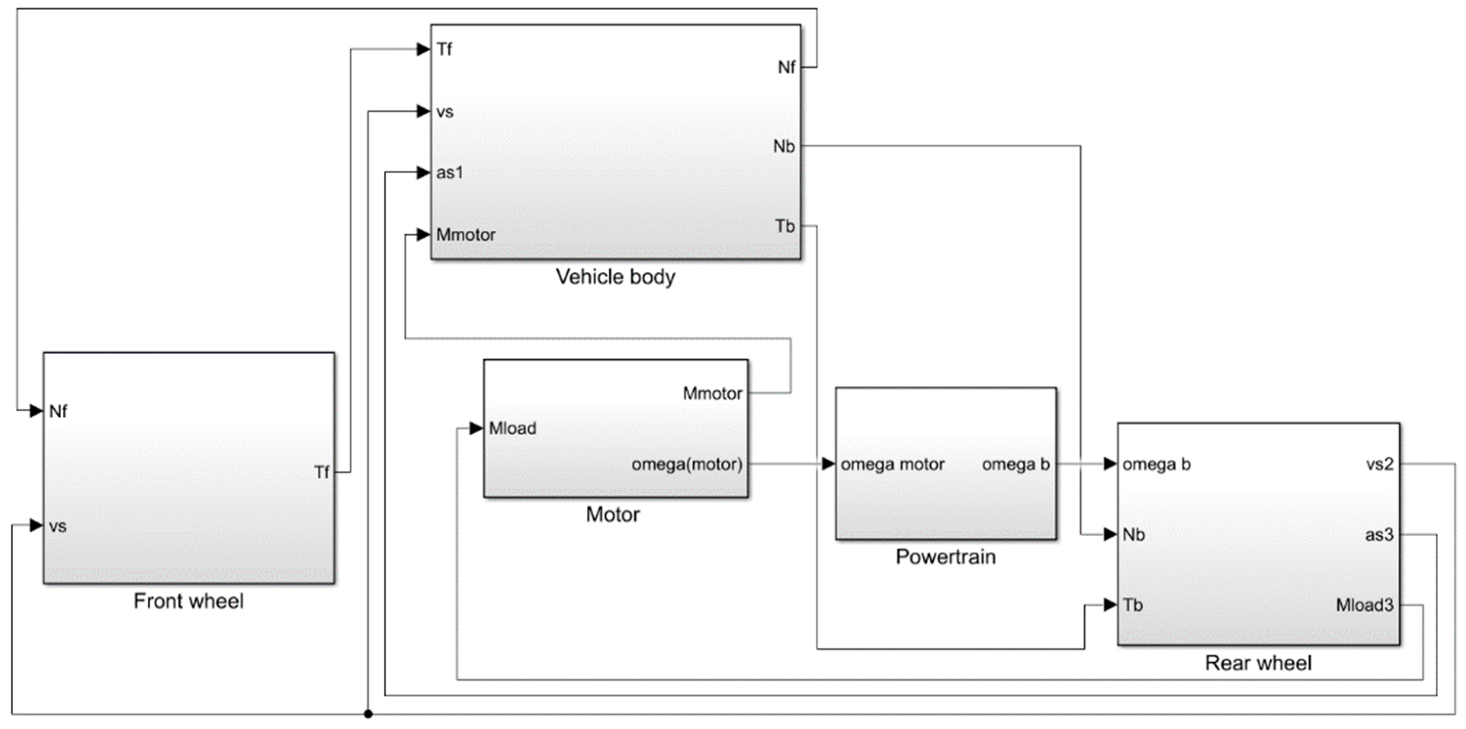
3. Brief Description of the Simulation Program

The applied simulation program [3] is based on the vehicle dynamics model presented in Figure 3 [3]. In the model, the car is divided into four structural units. These units are the driven rear wheels with the rotating machine parts connected to them (Unit 1), the freely rotating front wheels with the rotating machine parts connected to them (Unit 2), the body of the car including the stator of the electric motor (Unit 3), and the rotor of the electric motor (Unit 4).

Regarding the modelled vehicle in [3], the rear wheels are connected to the electric motor through a chain drive. The mathematical connection between $M_{wheel}$ and $M_{motor}$ is given by the Equation (9):

$$M_{wheel}=-\mathrm{ƞ}·i_{12}·M_{motor}$$

(9)

$$\mathrm{where}{i}_{12}=\frac{z_2}{z_1}$$

(10)

The meaning of the notations in Figure 3 and in Equations (9) and (10) can be found in the Nomenclature. To be able to simulate the electric motor, it must also be modelled. Regarding the prototype race car in [3], a series-wound DC motor was applied to drive the car. The developed model for this motor [3] is presented in Figure 4.

Based on the models—presented in Figure 3 and Figure 4—dynamic and electromagnetic equations were written for the various structural units [3]. Based on the equations, a simulation program was developed in MATLAB/Simulink [3]. The modular structure of the simulation program is presented in Figure 5.

The simulation program is built up of five modules according to our dynamics model. The modules are: vehicle body (Module 3), front wheels and connected rotating machine parts (Module 2), rear (back) wheels and connected rotating machine parts (Module 1), motor (Module 4), and power transmission system (Module 5).

A detailed description of the internal structure and operation of each module can be found in reference [3].

The inputs of the program and its output functions are listed in the Nomenclature. The electromagnetic and dynamic characteristics of the applied electric motor ($R_{batt}$, $V_{batt}$, $R_{wire}$, $R_s$, $R_r$, $L_s$, $L_r$, $L_{sr}$, $J_r$, $M_{res}$) were measured previously [8,9], and the output functions ($I\left(t\right)$, $M_{motor}\left(t\right)$, ${\omega }_{motor}\left(t\right)$) of the motor simulation program module were validated by test measurements [9]. Some of the other vehicle parameters ($l$, $l_f$, $l_b$, $w$, $m_0$, $m_f$, $m_b$, $J_f$, $J_b$, $R$, $A$) were also measured [3], while the remaining ones ($\mathrm{ƞ}$, $C$) were approximated on the basis of literature data.

4. Description of the Optimization Methods

The basic concepts related to optimization can be found in reference [12]. These concepts are clarified below.

The race car can be described with a finite number of technical data. Data that cannot be modified during the optimization procedure, are called design parameters, while others are called design variables. Together, they unambiguously define the vehicle model.

The introduction of design parameters is necessary because in most cases not all the data of the vehicle can be chosen freely. This may be due to the fact that the competition rules make restrictions (or fix the value) on certain data, or other practical or economic reasons (such as the use of an existing vehicle chassis, motor, or other vehicle components), or we may simply know the optimal value of a given technical data.

The design variables are categorized as mathematically continuous or discrete. It is usually easier to work with continuous design variables (since they can take any value in a given interval), but in certain situations (for example, if we need to select a rim for our car from the available sizes), you must use discrete design variables. In the intermediate case, when we know that we are looking for the value of a design variable in a discrete set containing a large number of elements (e.g., chain gear ratio selection), we talk about pseudo-discrete design variables. In this case, we solve the problem by considering the design variable to be continuous and then finding the most suitable discrete value closest to it.

The given fixed values of the design variables and parameters define a possible vehicle construction. This construction may be suitable for the designer, or it may also be possible that it does not meet the functional or other requirements. The conditions that the given construction must meet are called optimization conditions. These can be, for example, geometric optimization conditions, such as the minimum and maximum required track or wheelbase of the race car, or conditions related to the technical implementation, such as the minimum number of sprocket teeth in a chain drive, below which the chain drive cannot work. A construction that satisfies all the optimization conditions is called a permissible construction.

There are usually a large or infinite number of constructions that meet the optimization conditions. To select the optimal vehicle construction, we interpret an objective function on the set of design variables, the value of which is a quantity (metric) characteristic of the vehicle (for example, the time required to cover a given distance or reach a given speed, energy consumption, or top speed), based on which metric the designer prefers, one construction will be selected over another. In most cases, we formulate the optimization problem as the minimization of the objective function. The selection of the objective function has a significant effect on the whole optimization process, and thus, on the resulting optimal construction. We have the option of simultaneously interpreting several objective functions, but we recommend this only if the interpretation of one objective function is not sufficient and the objective functions do not contradict each other.

The simulation program presented in Section 3 can be used for optimization purposes in two ways: firstly, it helps to design a new vehicle. In this first case, only certain technical data (design parameters) have a given fixed value, for example, satisfying the competition rules. For the other technical data (design variables) we must find the optimal values, which are the most suitable for the given competition task (e.g., 100 m drag race). Secondly, it helps to prepare an existing vehicle for a given competition task. In this second case, we can vary or adjust only a few of the vehicle’s technical data. In both cases, using the simulation program and the optimization procedure, the possibility of successful racing can be significantly increased, and a lot of time and cost can be saved.

In the following, we present the applied optimization methods, together with the necessary program codes that were developed in MATLAB.

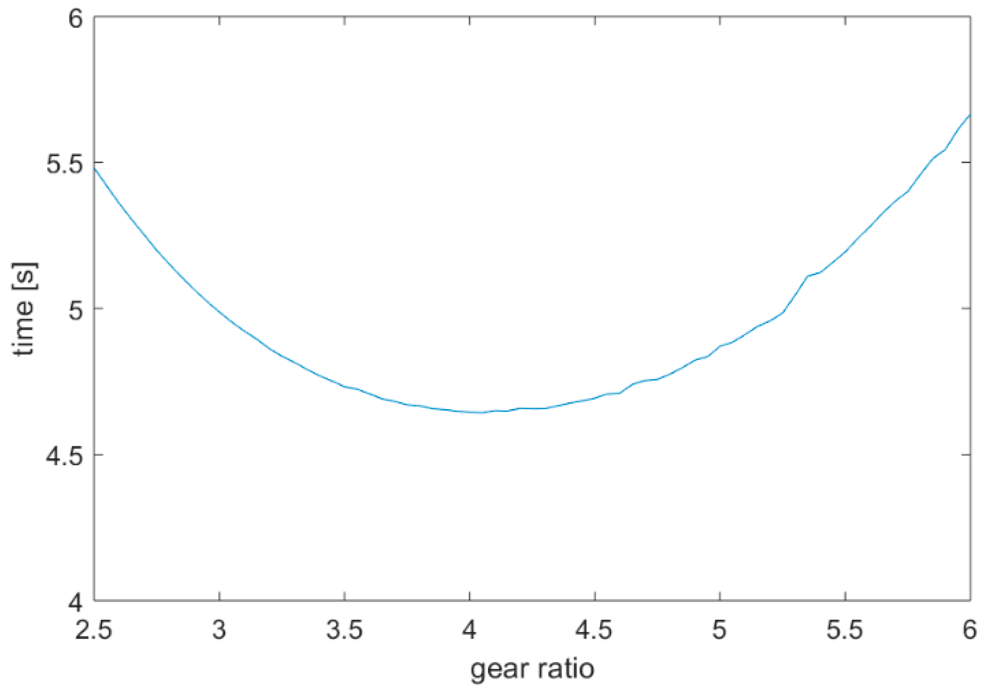
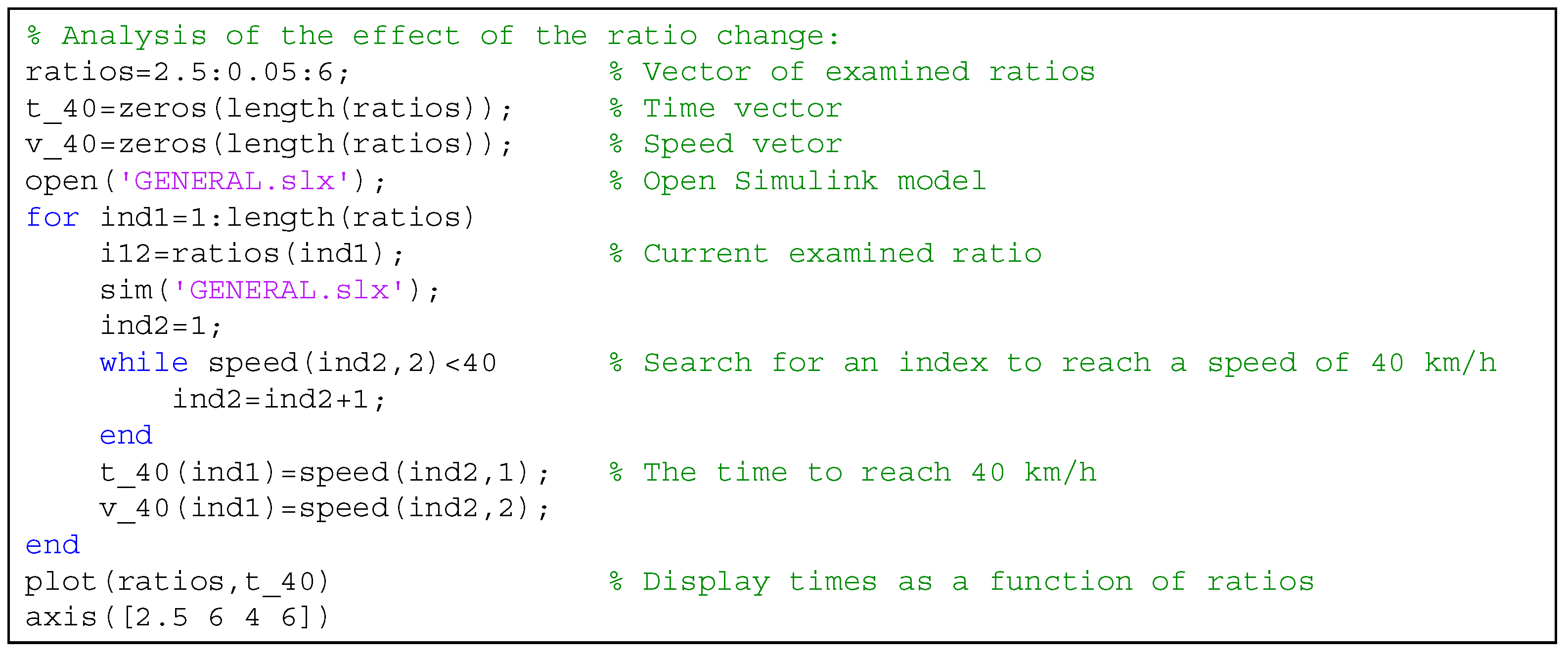
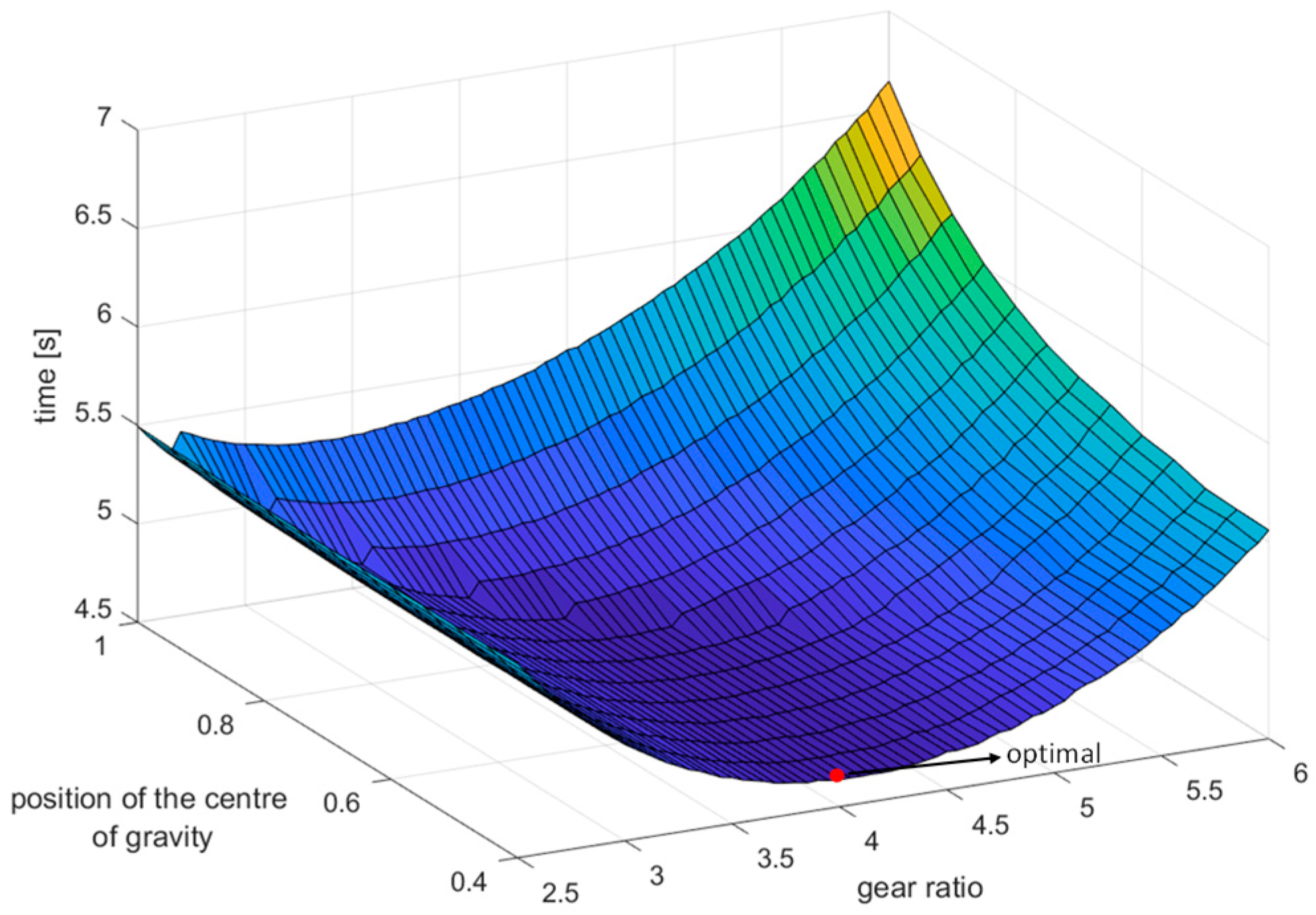
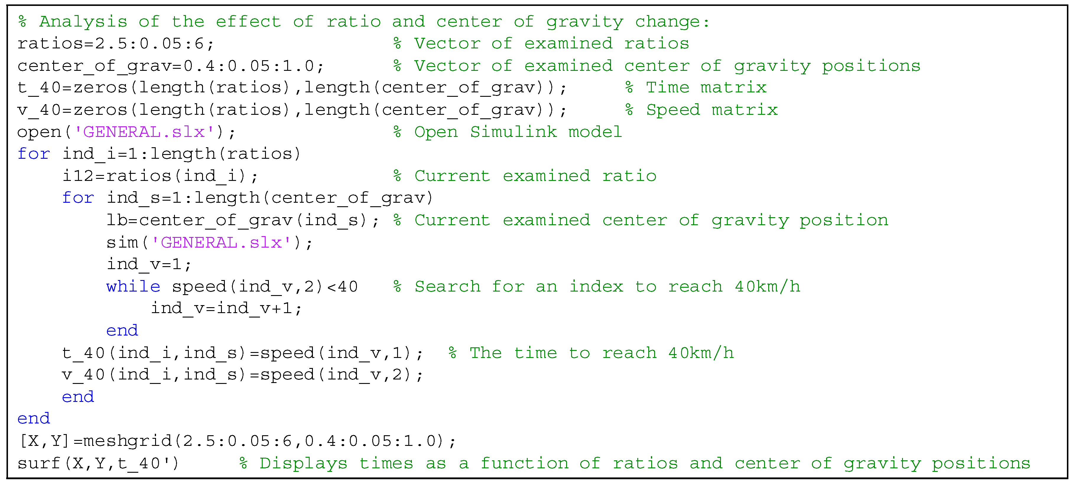
4.1. Approximation of the Optimal Technical Data Using a “Graphical Method”

In technical practice, it often happens that we search for the optimum with only one or two design variables, and the objective function has a “smooth” behavior, free of discontinuities or sudden changes. In this case, instead of computationally demanding optimization methods, we have the option of using a simpler “graphical method”. In this procedure, we generate a uniform “grid” on the space of design variables and calculate the values of the objective function at the grid points. Due to the nature of the task, the values of the objective function can be represented on one- or two-variable diagrams and the optimum can be read with a good engineering approximation. Of course, this procedure cannot be used in the case of a higher-dimensional design variable space or a highly complex objective function.

If we intend to optimize only one of the variables (for example, the gear ratio in the chain drive) then the objective function is a univariate function. Let the optimization problem be to find the optimal value of the gear ratio ($i_{12}$) at which a speed of 40 km/h can be reached by the race car in the shortest possible time ($t$). In this problem the design variable is the gear ratio, and the objective function is function $t\left(i_{12}\right)$. Applying our simulation program, we calculate the velocity–time function of the vehicle at different gear ratios and read the time required to reach a speed of 40 km/h. After that, the above time is plotted as a function of the gear ratio (Figure 6), and then the approximate value of the optimal gear ratio, corresponding to the minimum time, is read from the graph.

Since we have to run the program for many different gear ratios, we automated the process with the application of a self-developed MATLAB code (Figure 7).

In the MATLAB code above, we first specify the gear ratio range and the step size which are [2.5; 6] and 0.05, respectively. After that, we run the simulation program with every gear ratio value one by one. For this, we use a for loop in the program code. After that, the program records the times required to reach 40 km/h for each run and then plots them as a function of the corresponding gear ratios.

If we intend to optimize two of the variables, then the objective function is a bivariate function. In this case, the procedure presented previously for a univariate function can still be used. Let the optimization problem be to find the optimal values of the gear ratio and center-of-mass position ($l_b$) at which a speed of 40 km/h is reached by the car in the shortest possible time. Variable $l_b$ is the distance of the centre of mass of the vehicle from the rear shaft, and its value can be varied in the [0.4; 1] m range. Applying our simulation program, we calculate the velocity–time function of the vehicle at the different center-of-mass position and gear ratio pairs and read the time required to reach a speed of 40 km/h. After that, the above time is plotted as a function of the center-of-mass position and gear ratio pairs (Figure 8). Finally, the approximate center-of-mass position and gear ratio, corresponding to the minimum time, are read from the graph.

Based on Figure 8, the optimal values of the center of mass and the gear ratio are approximately 0.4 m and 4. The MATLAB program code (Figure 9) developed to automate the process is similar to the one in Figure 7. The only difference is that here two loops are used.

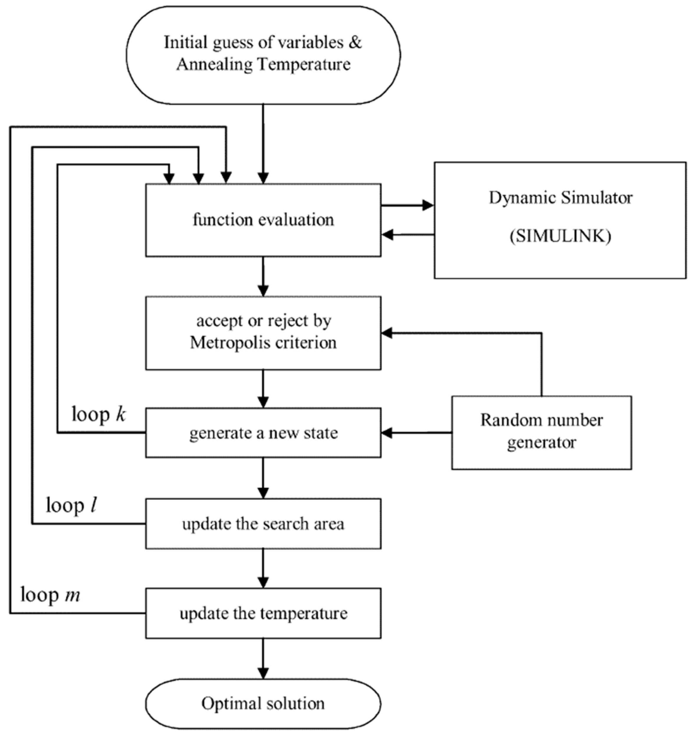
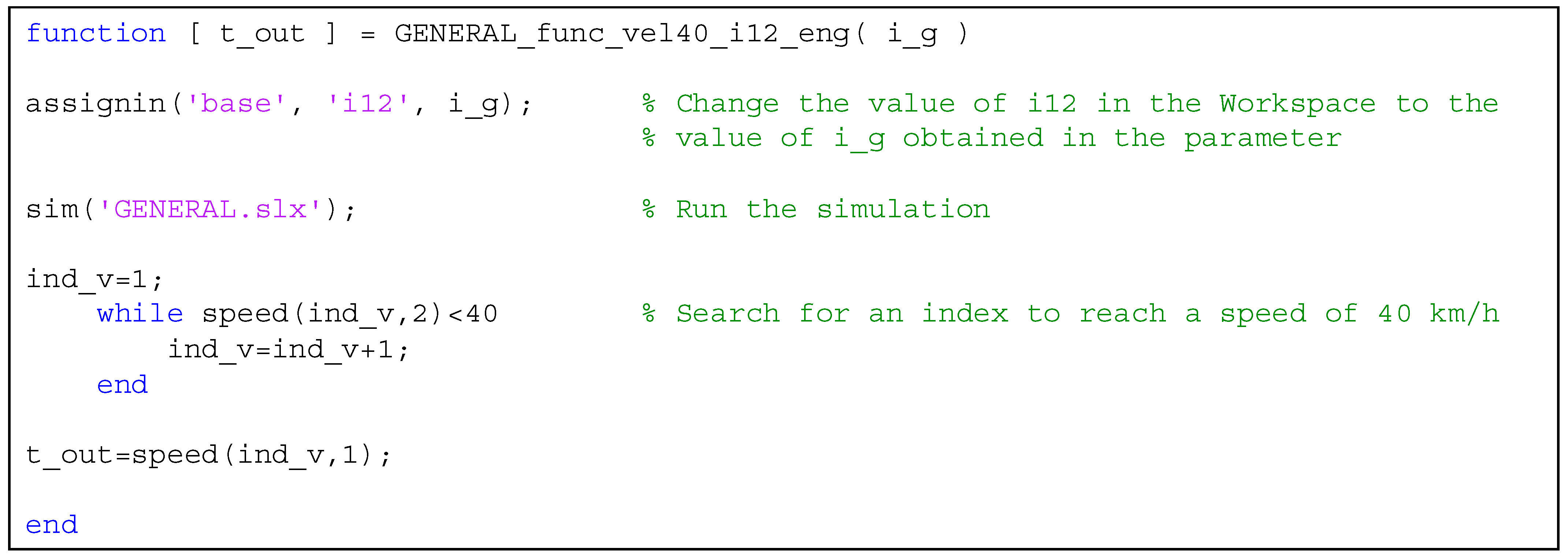
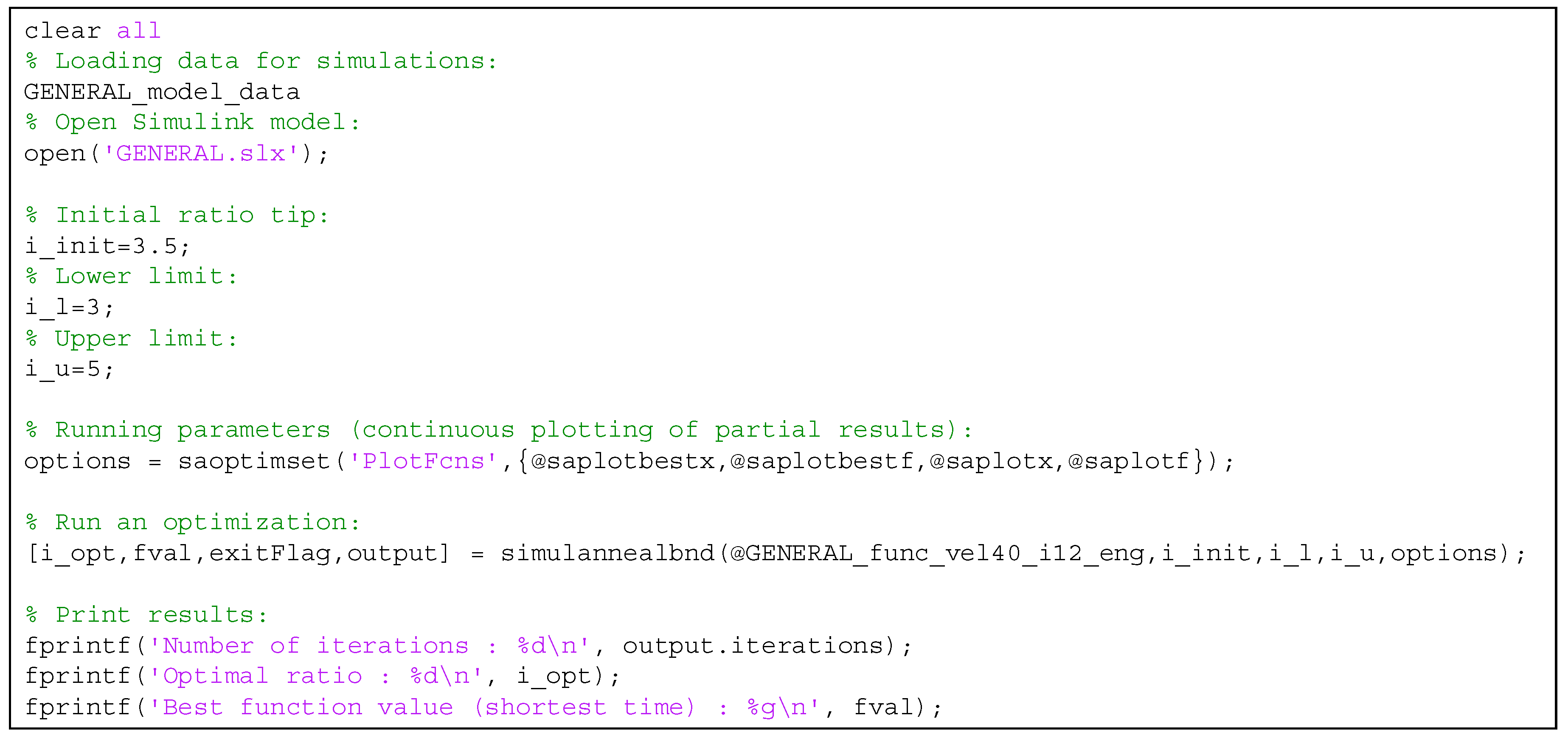
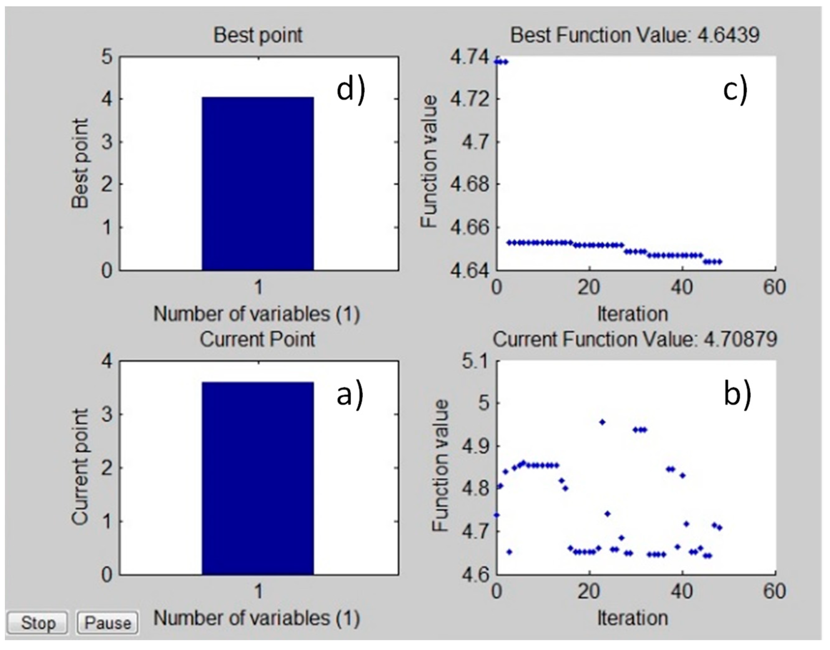
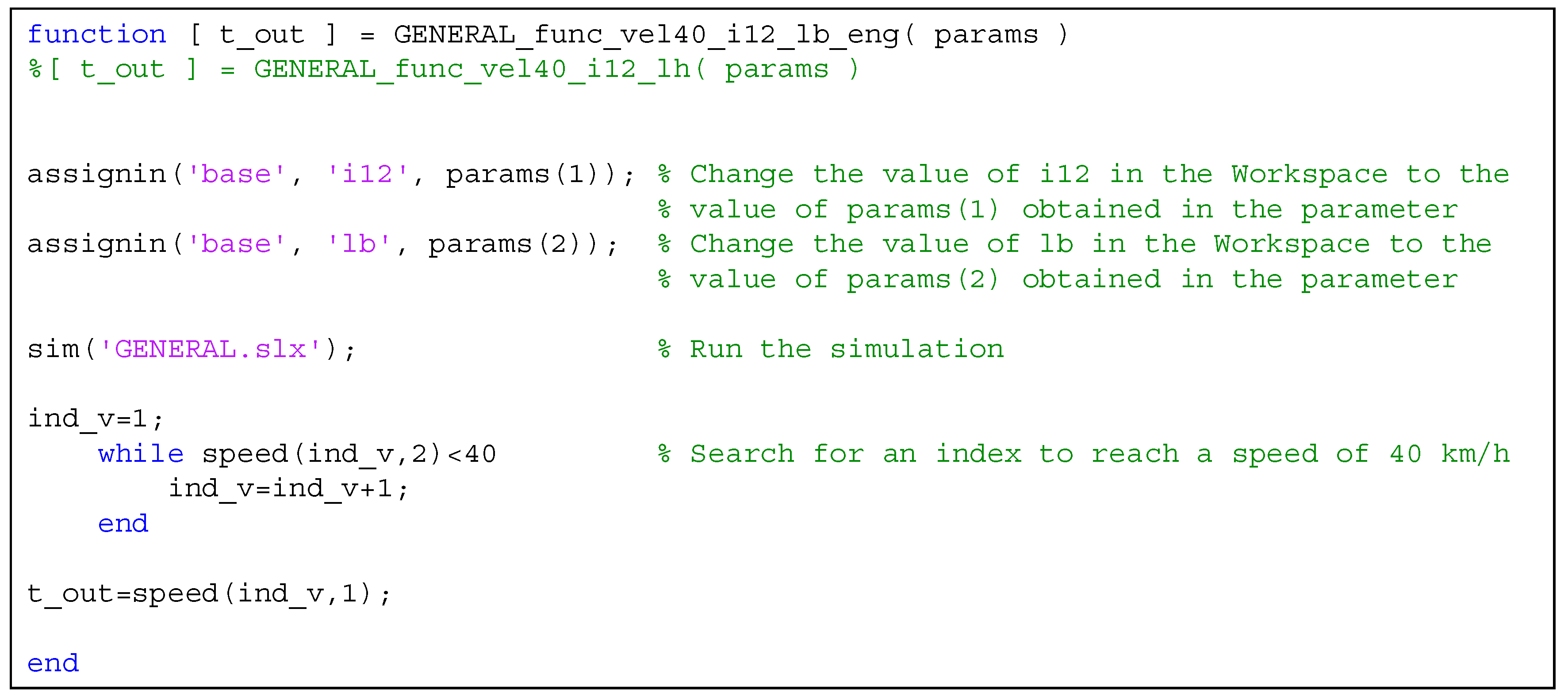
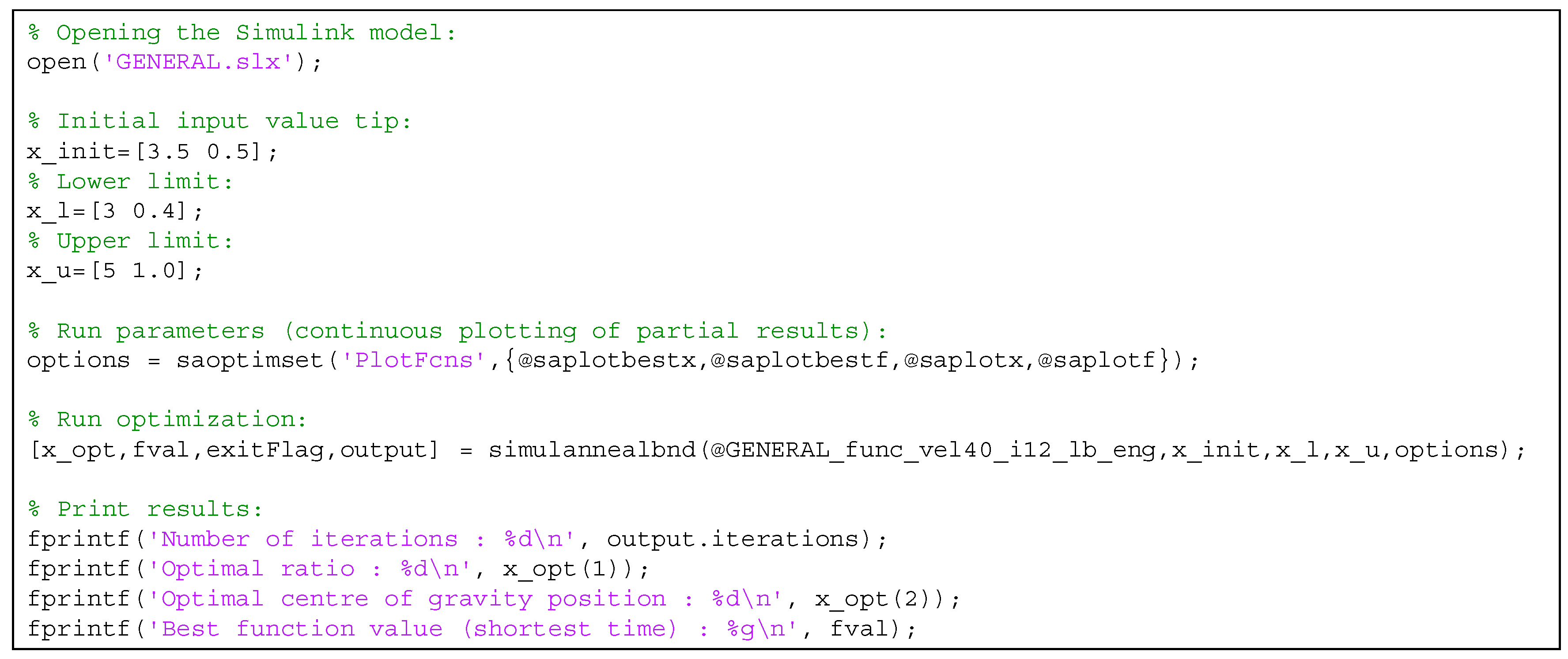
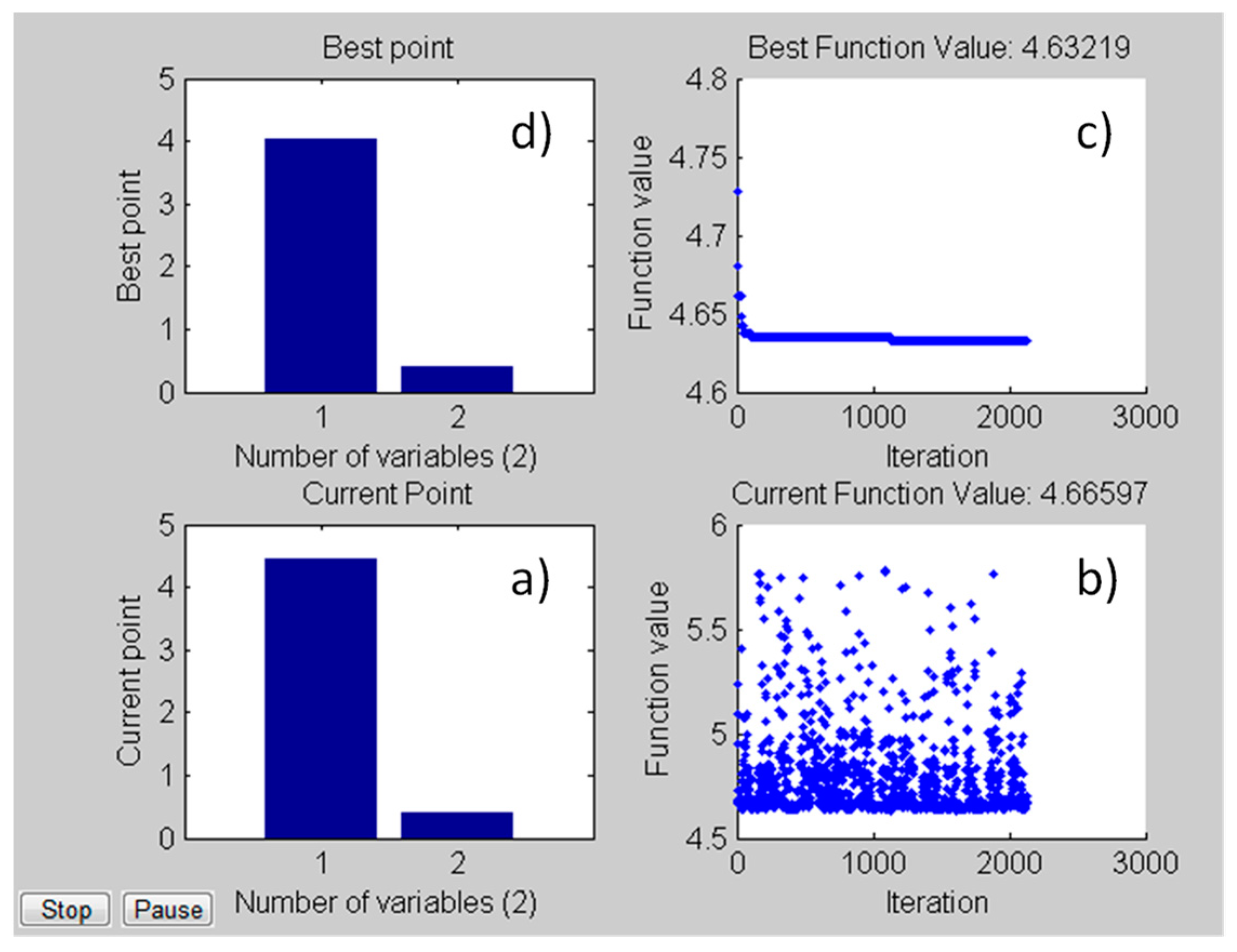
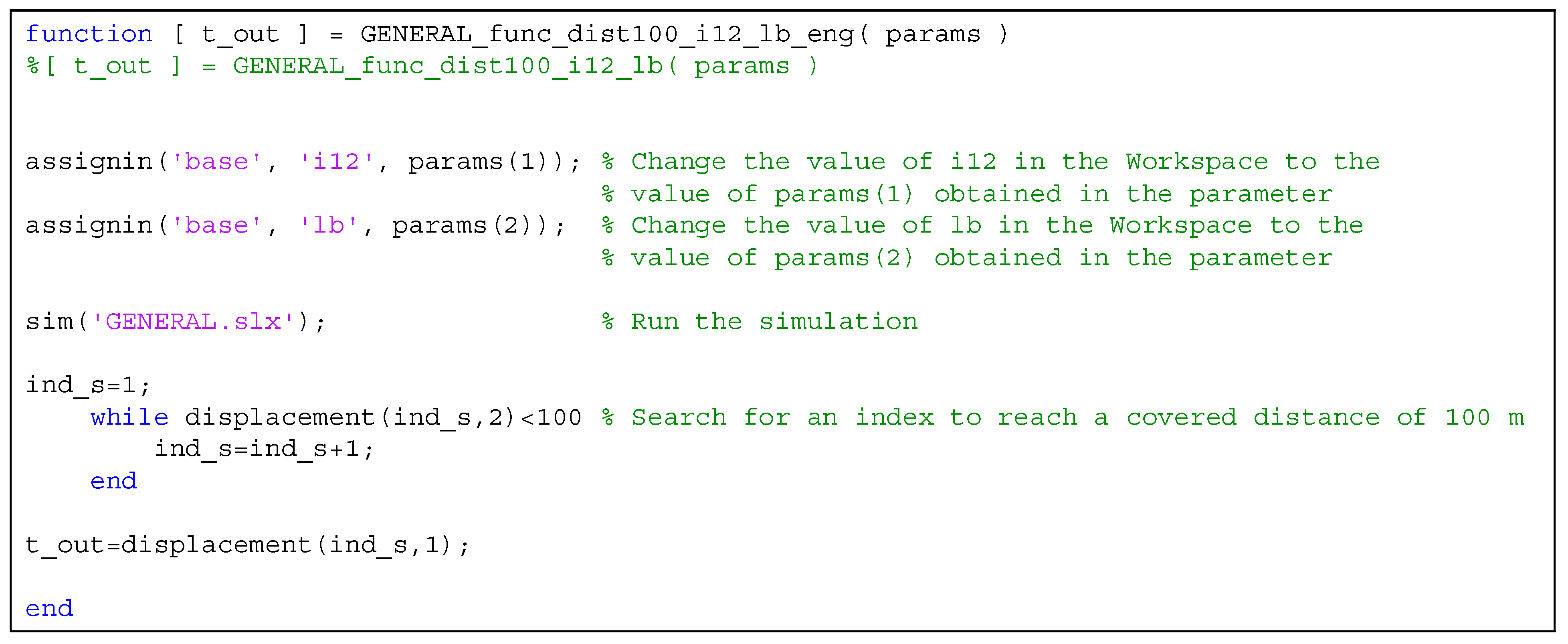
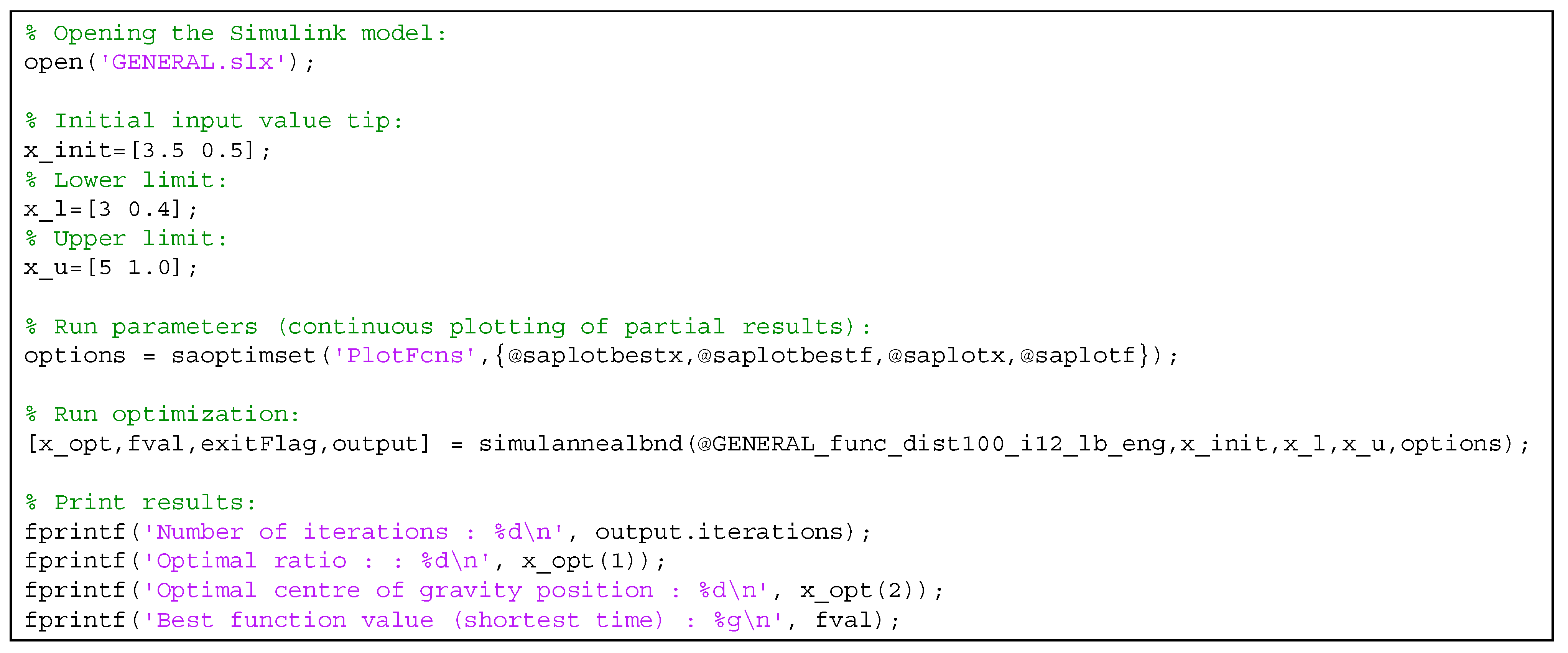
4.2. Determination of the Optimal Technical Data Using Simulated Annealing

For three or more variables, or when greater accuracy is required, we can no longer use the graphical method, instead we can use the stochastic method simulated annealing (SA). To realize the optimization, we used the simulated annealing function (simulannealbnd) in the Global Optimization Toolbox within MATLAB, which based on the general method of simulated annealing, described in Section 2. The above-mentioned MATLAB function uses a variant of SA which is the adaptive simulated annealing (ASA) [16]. In this variant (ASA), the algorithm parameters that control temperature scheduling and random-step selection, are set automatically. The values of the above parameters in the traditional version (SA) are usually adjusted by the user, based on their own experience, as was previously mentioned in Section 2. This is a significant disadvantage of traditional SA compared to ASA. During the optimization we used the default settings in MATLAB, in which the step length equals the current temperature, and direction is uniformly random. The current temperature is calculated from the initial temperature applying the formula $T=T_0·{0.95}^m$, where $m$ denotes the annealing parameter, which is the same as the iteration number.

As an example, we first show the application of simulated annealing in the case of one design variable. The task is the same as in Section 4.1, namely, to determine the optimal gear ratio of the race car [3], with which a speed of 40 km/h can be reached in the shortest possible time. Regarding the objective, first, it is necessary to create a MATLAB function, which calculates the time required to reach 40 km/h speed at different gear ratios ($i_{12}$). The program code that was developed for this is shown in Figure 10.

After that, the optimization program code is created (Figure 11), applying simulated annealing, using the MATLAB function presented in Figure 10.

Comparing this result with the one obtained by the graphical method, it can be seen that they are equal to a good approximation.

The optimization program code determines the minimum time required to reach 40 km/h speed and the value of the corresponding optimal gear ratio. While the program is running, the actual values can be monitored in real-time in four windows (Figure 12).

In the following, we apply simulated annealing for the optimization of two design variables of the same car. These variables are the gear ratio and the position of the center of mass of the car. Currently, in the case of the above-mentioned car, we can vary only these parameters easily, and they have a significant effect on the dynamic characteristics of the car. Thus, we decided to optimize the above parameters for the following two objectives:

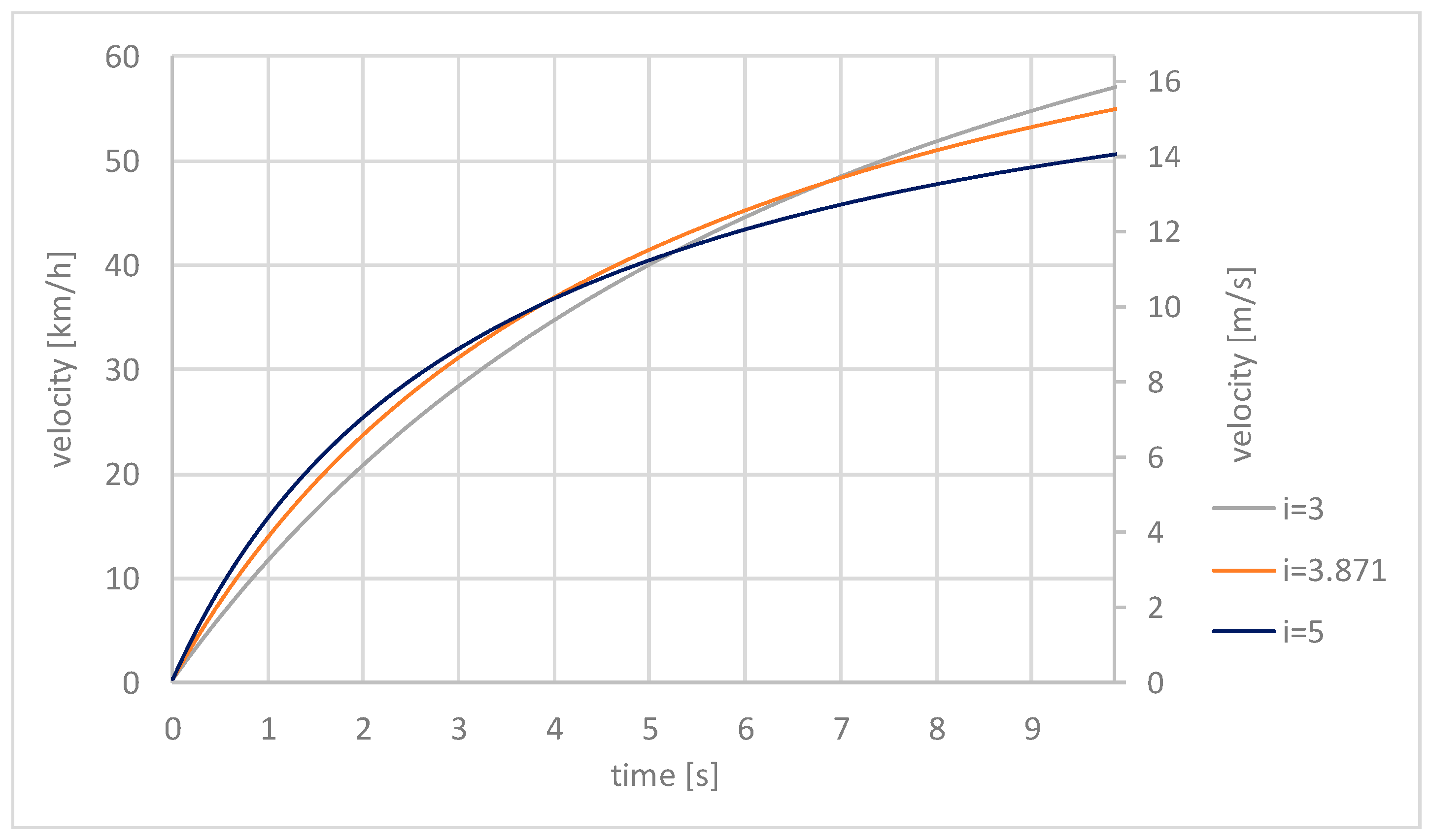
• Reaching 40 km/h speed in the shortest possible time;
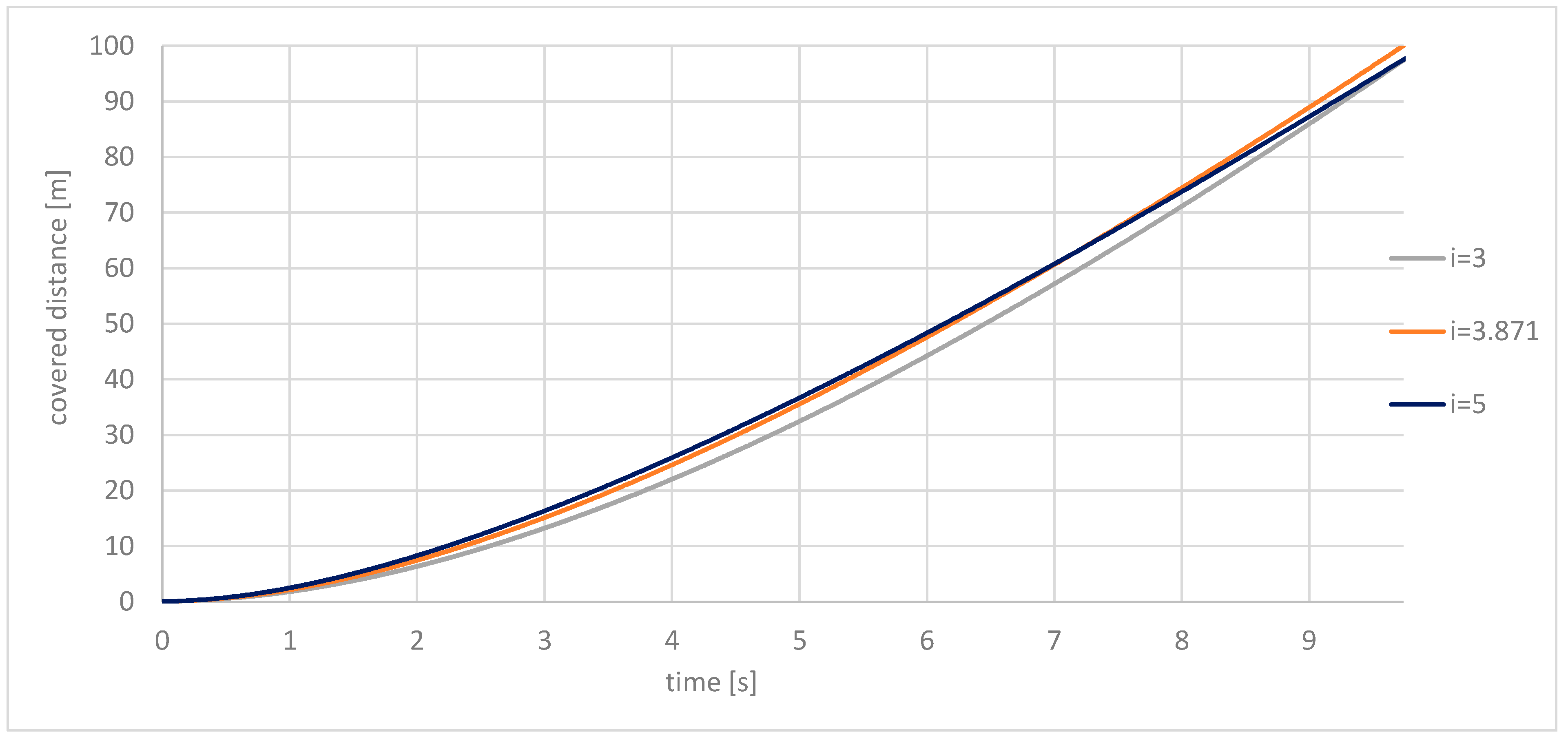
• Covering a distance of 100 m from a standing position in the shortest possible time (drag race).

Regarding the first objective, good acceleration in the 0–40 km/h speed range is an important factor for driving on a racetrack with many sharp turns. (The top speed of the car is between 60 and 80 km/h, depending on the settings of the technical data.) To realize the optimization, regarding the first objective, first, it is necessary to create a MATLAB function that calculates the time required to reach 40 km/h speed at different gear ratios ($i_{12}$) and the position of the centre of mass ($l_b$) pairs. The program code that was developed for this is shown in Figure 13.

After that, the optimization program code is created (Figure 14), applying simulated annealing, using the MATLAB function presented in Figure 13.

The optimization program code determines the minimum time required to reach 40 km/h speed and the values of the corresponding optimal gear ratio and center-of-gravity position. While the program is running, the actual values can be monitored in real-time in four windows (Figure 15).

Regarding the second objective (drag race), for the optimization, first, it is necessary to create a MATLAB function, which calculates the time required for the car to travel 100 m at different gear ratio ($i_{12}$) and the position of the center-of-gravity ($l_b$) pairs. The program code developed for this is shown in Figure 16.

After that, the optimization program code is created (Figure 17), applying simulated annealing, using the MATLAB function presented in Figure 16.

While the program is running, the actual values can be monitored in real-time, similarly to the previous case. At the end of the run, the optimal values are also displayed in a MATLAB Command Window. In the case of the analyzed race car, the minimum time is 9.74 s, and the optimal values of the gear ratio and the center-of-gravity position are 3.871 and 0.423 m, respectively.

After that, the simulation program was run on the [0; 9.74] s time interval with the optimal gear ratio and center-of-gravity position pairs obtained at objective 2 (3.871 and 0.423 m, respectively), as well as with two other, non-ideal variable pairs (3 and 0.423 m, 5 and 0.423 m). Figure 18 shows the covered distance–time functions of the vehicle applying the above input parameters.

Based on the figure above, it can be concluded that, when applying the optimal gear ratio (3.871), the vehicle travels approximately 2.5 m more in 9.74 s than when applying the other two gear ratios (3 and 5). From a different point of view, this means that using the optimal gear ratio, the distance of 100 m can be covered 0.3 s faster than using the other two gear ratios.

Figure 19 shows the velocity–time functions of the vehicle applying the same input parameters as in the case of Figure 18.

Despite the fact, that after 9.74 s the highest speed can be reached using gear ratio $i_{12}$ = 3, this will not be optimal for covering the 100 m distance in the shortest time.

Figure 20 shows the energy consumption of the race car as a function of time, applying the same gear ratios as in the case of Figure 18 and Figure 19.

The energy consumed by the car was calculated as the definite integral from 0 to t of the product of the battery’s terminal voltage and the intensity of the electric current flowing through it.

Despite the fact, that in the first 9.74 s, the lowest energy consumption can be reached using gear ratio $i_{12}$ = 5, this will not be optimal for covering the 100 m distance in the shortest time.

Depending on the type of competition (i.e., what the specific competition task is), the optimal value for a given technical data may be different. As we have seen, depending on whether the goal is the lowest possible energy consumption, the maximum speed achieved in a given time, or covering a given distance in the shortest time, the value of the optimal gear ratio is different.

Finally, let us cite two examples. The first one is the “acceleration” race of the world-famous Formula Student race, where the task for the car is to complete the 75 m track in the shortest possible time from a standstill. The second is the international Shell-ECO Marathon competition, where the task is to complete the given race distance with the lowest energy consumption, under the condition that the average speed for the entire race distance must be at least 25 km/h. Applying our method, we can find the optimal values of technical data at which the best performance can be achieved regarding the above competition tasks.

5. Conclusions

In this publication, we have presented novel procedures for optimizing the technical parameters of prototype race cars for specific competition tasks, using our vehicle dynamics simulation program. Two types of optimization procedures were presented.

The first one is a graphical method, which can be used in case of one or two design variables. Due to its simplicity, this method can be used effectively, and its accuracy, in most cases, is adequate from an engineering point of view. Therefore, applying our simulation program, and having at the maximum, two variables, the application of a complex optimization procedure is usually not justified.

In this publication the graphical method was applied to an existing prototype race car to optimize one and two of its parameters to a given competition tasks. These parameters were the gear ratio in the chain drive and the horizontal distance of the center of gravity from the back shaft.

The second procedure is an application of simulated annealing to optimize the same parameters of the car for two different competition tasks. One of these tasks was the same as the one in the graphical method. Applying simulated annealing, the optimal values can be calculated directly, and it can be also applied for three or more variables, or when greater accuracy is required.

If we want to achieve the same accuracy with the graphical method and the simulated annealing, then in the case of the graphical method we have to run our simulation program many more times than in the case of the simulated annealing. As a result, simulated annealing is a more efficient method.

In case of adaptive simulated annealing—which is used by MATLAB—the algorithm parameters, that control temperature scheduling and random step selection, are adjusted automatically by the program. Additionally, the convergence of the algorithm is theoretically guaranteed starting from any initial parameter values. Thus, this is a robust optimization algorithm. With the graphical method, from the point of view of robustness, it can be a problem if we cannot read the exact location of the optimum after running the program once, so the program must be run again with a smaller step size.

The obtained optimal values for the analyzed two parameters were the same, with a good approximation when applying the graphical method and simulated annealing. The simulation results showed, that using the optimal gear ratio (3.871), the distance of 100 m can be covered 0.3 s faster than using other non-ideal gear ratios (3 and 5).

In general, it can be concluded that our vehicle dynamics simulation program, supplemented with the described optimization procedures, can be effectively used to optimize the technical data of an existing or designed prototype race car for various racing tasks. Knowing the optimal technical parameters significantly increases the possibility that a given prototype race car successfully competes in domestic or international competitions. Additionally, there is no need to manufacture many unnecessary machine parts and test them under real conditions. This saves us a lot of time and significantly reduces our costs.

In the future, in the case of race cars produced at the Faculty of Engineering of the University of Debrecen, the dynamic modelling, simulation, and determination of the optimal technical parameters of a given vehicle concept will be a natural part of the design process. We hope that this will greatly contribute to competing successfully, and thus to the success of the Faculty of Engineering of the University of Debrecen.

References

1. Gy, J. A Pneumobil Versenyek és az Oktatás—A Felkészülés Tanári Szemmel, Debreceni Műszaki Közlemények; University of Debrecen: Debrecen, Hungary, 2011; Volume 10, pp. 35–40. [Google Scholar]
2. Gábora, A.; Sziki, G.Á.; Szántó, A.; Varga, T.A.; Magyari, A.; Balázs, D. Prototype battery electric car development for Shell-ECO-Marathon® competition. In Proceedings of the XXII International Conference of Young Engineers, Kolozsvár, Romania, 23 March 2017; pp. 167–170. [Google Scholar]
3. Szántó, A.; Hajdu, S.; Sziki, G. Dynamic Simulation of a Prototype Race Car Driven by Series Wound DC Motor in Matlab- Simulink. Acta Polytech. Hung. 2020, 17, 103–122. [Google Scholar] [CrossRef]
4. Pálinkás, S. Influence of Speed to Rolling Resistance Factor in Case of Autobus. In Vehicle and Automotive Engineering 4: Select Proceedings of the 4th VAE2022, Miskolc, Hungary; Springer International Publishing: Cham, Switzerland, 2011; pp. 157–164. [Google Scholar]
5. Pálinkás, S.; Tóth, Á. Development of a measurement method to determine rolling resistance. IOP Conf. Series Mater. Sci. Eng. 2022, 1237, 012013. [Google Scholar] [CrossRef]
6. Szíki, G.; Szántó, A.; Mankovits, T. Dynamic modelling and simulation of a prototype race car in MATLAB/Simulink applying different types of electric motors. Int. Rev. Appl. Sci. Eng. 2021, 12, 57–63. [Google Scholar] [CrossRef]
7. Szántó, A.; Szántó, A.; Sziki, G.Á. Review of the modelling methods of series wound DC motors. Műszaki Tudományos Közlemények 2020, 13, 166–169. [Google Scholar] [CrossRef]
8. Sziki, G.; Sarvajcz, K.; Kiss, J.; Gál, T.; Szántó, A.; Gábora, A.; Husi, G. Experimental investigation of a series wound DC motor for modeling purpose in electric vehicles and mechatronics systems. Measurement 2017, 109, 111–118. [Google Scholar] [CrossRef] [Green Version]
9. Szántó, A.; Kiss, J.; Mankovits, T.; Szíki, G. Dynamic Test Measurements and Simulation on a Series Wound DC Motor. Appl. Sci. 2021, 11, 4542. [Google Scholar] [CrossRef]
10. Szántó, A.; Ádámkó, É.; Juhász, G.; Sziki, G.Á. Simultaneous measurement of the moment of inertia and braking torque of electric motors applying additional inertia. Measurement 2022, 204, 112135. [Google Scholar] [CrossRef]
11. Sziki, G.; Szántó, A.; Kiss, J.; Juhász, G.; Ádámkó, É. Measurement System for the Experimental Study and Testing of Electric Motors at the Faculty of Engineering, University of Debrecen. Appl. Sci. 2022, 12, 10095. [Google Scholar] [CrossRef]
12. Rao, S.S. Engineering Optimization Theory and Practice; John Wiley & Sons Inc.: London, UK, 2019; pp. 694–702. [Google Scholar]
13. Kirkpatrick, S.; Gelatt, C.D., Jr.; Vecchi, M.P. Optimization by simulated annealing. Science 1983, 220, 671–680. [Google Scholar]
14. Kirkpatrick, S. Optimization by simulated annealing: Quantitative studies. J. Stat. Phys. 1984, 34, 975–986. [Google Scholar] [CrossRef]
15. Faber, R.; Jockenhövel, T.; Tsatsaronis, G. Dynamic optimization with simulated annealing. Comput. Chem. Eng. 2005, 29, 273–290. [Google Scholar] [CrossRef]
16. Ingber, L. Adaptive simulated annealing (ASA): Lessons learned. Control. Cybern. 1996, 25, 33–54. [Google Scholar]
17. Kapusi, T.P.; Erdei, T.I.; Husi, G.; Hajdu, A. Application of Deep Learning in the Deployment of an Industrial SCARA Machine for Real-Time Object Detection. Robotics 2022, 11, 69. [Google Scholar] [CrossRef]
18. Erdei, T.I.; Krakó, R.; Husi, G. Design of a Digital Twin Training Centre for an Industrial Robot Arm. Appl. Sci. 2022, 12, 8862. [Google Scholar] [CrossRef]
19. Erdei, T.I.; Husi, G. Singularity measurement in the Cyber-physical and intelligent robot systems laboratory. Int. Rev. Appl. Sci. Eng. 2020, 11, 82–87. [Google Scholar] [CrossRef]
20. Erdei, T.; Molnár, Z.; Obinna, N.C.; Husi, G. A Novel Design of an Augmented Reality Based Navigation System & its Industrial Applications. Acta IMEKO 2018, 7, 57–62. [Google Scholar] [CrossRef] [Green Version]
21. Adamko, E.; Szemes, P.T.; Niitsuma, M. Investigation on the heating system of the mechatronics research center building using olap technology. Environ. Eng. Manag. J. 2014, 13, 2733–2742. [Google Scholar] [CrossRef]
22. Ádámkó, É.; Szemes, P.T. Evaluation of consumer Behavior in the building mechatronics research centre. Recent Innov. Mechatron. Recent Innov. Mechatron. (RIiM) Int. J. Mechatron. Sci. 2014, 1–5. [Google Scholar]
23. Li, P.; Löwe, K.; Arellano-Garcia, H.; Wozny, G. Integration of simulated annealing to a simulation tool for dynamic optimization of chemical processes. Chem. Eng. Process. 2000, 39, 357–363. [Google Scholar] [CrossRef]
24. Beltran, A.; Rumbo, J.; Azcaray, H.; Santiago, K.; Calixto, M.; Sarmiento, E. Simulation and control of the speed and electromagnetic torque of a three-phase induction motor: An electric vehicles approach. Iberoam. Mag. Auto-Matic Ind. Inform. 2019, 16, 308–320. [Google Scholar]
25. Nguyen, T.T.V.; Vo, T.M.N. Centrifugal pump design: An optimization. Eurasia Proc. Sci. Technol. Eng. Math. 2022, 17, 136–151. [Google Scholar] [CrossRef]
26. Huynh, N.-T.; Nguyen, T.V.T.; Tam, N.T.; Nguyen, Q.-M. Optimizing Magnification Ratio for the Flexible Hinge Displacement Amplifier Mechanism Design. In Proceedings of the 2nd Annual International Conference on Material, Machines and Methods for Sustainable Development (MMMS2020), Nha Trang, Vietnam, 12–15 November 2020; pp. 769–778. [Google Scholar] [CrossRef]
27. Wang, C.-N.; Yang, F.-C.; Vo, N.T.M.; Nguyen, V.T.T. Enhancing Lithium-Ion Battery Manufacturing Efficiency: A Comparative Analysis Using DEA Malmquist and Epsilon-Based Measures. Batteries 2023, 9, 317. [Google Scholar] [CrossRef]
28. Zadeh, L.A. Fuzzy logic. Computer 1988, 21, 83–93. [Google Scholar] [CrossRef]
29. Adeli, H.; Sarma, K.C. Cost Optimization of Structures: Fuzzy Logic, Genetic Algorithms, and Parallel Computing; John Wiley & Sons: Hoboken, NJ, USA, 2006. [Google Scholar]
30. Kim, J.; Kasabov, N. HyFIS: Adaptive neuro-fuzzy inference systems and their application to nonlinear dynamical systems. Neural Netw. 1999, 12, 1301–1319. [Google Scholar] [CrossRef] [PubMed]
31. Elbaz, K.; Shen, S.-L.; Zhou, A.; Yuan, D.-J.; Xu, Y.-S. Optimization of EPB Shield Performance with Adaptive Neuro-Fuzzy Inference System and Genetic Algorithm. Appl. Sci. 2019, 9, 780. [Google Scholar] [CrossRef] [Green Version]
32. Karna, S.K.; Sahai, R. An overview on Taguchi method. Int. J. Eng. Math. Sci. 2012, 1, 11–18. [Google Scholar]
33. Krishankant, J.T.; Bector, M.; Kumar, R. Application of Taguchi method for optimizing turning process by the effects of machining parameters. Int. J. Eng. Adv. Technol. 2012, 2, 263–274. [Google Scholar]
34. Julong, D. Introduction to grey system theory. J. Grey Syst. 1989, 1, 1–24. [Google Scholar]
35. Li, Y.X.; Yang, J.G.; Gelvis, T. Optimization of measuring points for machine tool thermal error based on grey system theory. Int. J. Adv. Manuf. Technol. 2006, 35, 745–750. [Google Scholar] [CrossRef]
36. Rao, R.V.; Savsani, V.J.; Vakharia, D.P. Teaching–learning-based optimization: A novel method for constrained mechanical design optimization problems. Comput. Aided Des. 2011, 43, 303–315. [Google Scholar] [CrossRef]
37. Rao, R.V. Teaching-Learning-Based Optimization Algorithm; Springer International Publishing: Berlin/Heidelberg, Germany, 2016; pp. 9–39. [Google Scholar]
38. Sivanandam, S.; Deepa, S. Genetic Algorithm Optimization Problems. In Introduction to Genetic Algorithms; Springer: Berlin/Heidelberg, Germany, 2007; pp. 165–209. [Google Scholar] [CrossRef]
39. Wang, D.; Tan, D.; Liu, L. Particle swarm optimization algorithm: An overview. Soft Comput. 2018, 22, 387–408. [Google Scholar] [CrossRef]
40. Glover, F.; Kelly, J.P.; Laguna, M. Genetic algorithms and tabu search: Hybrids for optimization. Comput. Oper. Res. 1995, 22, 111–134. [Google Scholar] [CrossRef]
41. Miranda, M.H.; Silva, F.L.; Lourenço, M.A.; Eckert, J.J.; Silva, L.C. Vehicle drivetrain and fuzzy controller opti-mization using a planar dynamics simulation based on a real-world driving cycle. Energy 2022, 257, 124769. [Google Scholar] [CrossRef]
42. Eckert, J.J.; Santiciolli, F.M.; Silva, L.C.; Dedini, F.G. Vehicle drivetrain design multi-objective optimization. Mech. Mach. Theory 2021, 156, 104123. [Google Scholar] [CrossRef]
43. Eckert, J.J.; Silva, L.C.; Costa, E.S.; Santiciolli, F.M.; Dedini, F.G.; Corrêa, F.C. Electric vehicle drivetrain opti-misation. IET Electr. Syst. Transp. 2017, 7, 32–40. [Google Scholar]
44. Salvan, L.; Brüll, M.; Hollstein, A.; Medina, R.; Wilkins, S.; Avramis, N. Electric Drivetrain Optimization for 48V Urban Vehicles. In Proceedings of the 35th Electric Vehicle Symposium (EVS35), Sacramento, CA, USA, 11–14 June 2022; pp. 1–13. [Google Scholar]
45. Desai, C. Design and Optimization of Hybrid Electric Vehicle Drivetrain and Control Strategy Parameters Using Evolutionary Algorithms. Ph.D. Thesis, Concordia University, Mequon, WI, USA, 2010. [Google Scholar]
46. Lu, M.; Domingues-Olavarría, G.; Márquez-Fernández, F.J.; Fyhr, P.; Alaküla, M. Electric Drivetrain Optimization for a Commercial Fleet with Different Degrees of Electrical Machine Commonality. Energies 2021, 14, 2989. [Google Scholar] [CrossRef]
47. Tran, M.-K.; Akinsanya, M.; Panchal, S.; Fraser, R.; Fowler, M. Design of a Hybrid Electric Vehicle Powertrain for Performance Optimization Considering Various Powertrain Components and Configurations. Vehicles 2020, 3, 20–32. [Google Scholar] [CrossRef]
48. Zhang, P.; Chen, Y.; Lin, M.; Ma, B. Optimum Matching of Electric Vehicle Powertrain. Energy Procedia 2016, 88, 894–900. [Google Scholar] [CrossRef] [Green Version]
49. Li, C.; Cong, Z.; Zhang, B.; Jing, H. A Simulated Annealing algorithm based optimization for vehicle Powertrain Mounting System. In Proceedings of the 2015 5th International Conference on Information Science and Technology (ICIST), Changsha, China, 24–26 April 2015; IEEE: Piscataway, NJ, USA, 2015; pp. 10–13. [Google Scholar] [CrossRef]
50. Genc, M.O.; Kaya, N. Vibration Damping Optimization using Simulated Annealing Algorithm for Vehicle Powertrain System. Eng. Technol. Appl. Sci. Res. 2020, 10, 5164–5167. [Google Scholar] [CrossRef]
51. Ahssan, M.R.; Ektesabi, M.; Gorji, S. Evaluation of a Three-Parameter Gearshift Strategy for a Two-Speed Transmission System in Electric Vehicles. Energies 2023, 16, 2496. [Google Scholar]
52. Dokeroglu, T.; Sevinc, E.; Kucukyilmaz, T.; Cosar, A. A survey on new generation metaheuristic algorithms. Comput. Ind. Eng. 2019, 137, 106040. [Google Scholar] [CrossRef]
53. Feehery, W.F. Dynamic Optimization with Path Constraints. Ph.D. Thesis, Masachusetts Institute of Technology, Cambridge, MA, USA, 1998. [Google Scholar]
54. Corana, A.; Marchesi, M.; Martini, C.; Ridella, S. Minimizing multimodal functions of continuous variables with the “simulated annealing” algorithm. ACM Trans. Math. Softw. 1987, 13, 262–280. [Google Scholar] [CrossRef]
Figure 1. Flow chart of the general simulated annealing algorithm [15].
Applsci 13 08897 g001
Figure 2. The way of step length adjustment [15].
Applsci 13 08897 g002
Figure 3. The developed vehicle dynamics model for the prototype race car together with the forces and torques acting on its different structural units [3].
Applsci 13 08897 g003
Figure 4. The applied model for the simulation of the series-wound DC motor [3].
Applsci 13 08897 g004
Figure 5. The block diagram of the simulation program in MATLAB Simulink [3].
Applsci 13 08897 g005
Figure 6. The time that is necessary for reaching the 40 km/h speed as a function of the gear ratio.
Applsci 13 08897 g006
Figure 7. MATLAB code for automating the generation of the time vs. gear ratio function.
Applsci 13 08897 g007
Figure 8. The time that is necessary for reaching the 40 km/h speed as a function of gear ratio and center-of-gravity position.
Applsci 13 08897 g008
Figure 9. MATLAB program code for automating the generation of the function in Figure 8.
Applsci 13 08897 g009
Figure 10. The MATLAB code that was developed to calculate the time required to reach 40 km/h speed at different gear ratios ( i 12 ).
Applsci 13 08897 g010
Figure 11. The developed program code for the optimization applying simulated annealing.
Applsci 13 08897 g011
Figure 12. MATLAB windows for monitoring the parameter values in real-time. The first window (a) shows the current value of the gear ratio, the second one (b), the calculated times for the previously analyzed gear ratios, the third one (c), the smallest time vs. the number of iterations, and the fourth one (d), the optimal value of the gear ratio at which the time is minimum. At the end of the run, the optimal value is displayed in the MATLAB Command Window.
Applsci 13 08897 g012
Figure 13. The MATLAB code that was developed to calculate the time required to reach 40 km/h speed at different gear ratios ( i 12 ) and the position of the centre of gravity ( l b ) pairs.
Applsci 13 08897 g013
Figure 14. The developed program code for the optimization applying simulated annealing in the case of objective 1.
Applsci 13 08897 g014
Figure 15. MATLAB windows for monitoring the parameter values in real-time. The first window (a) shows the current values of the gear ratio and center-of-gravity position, the second one (b), the calculated times for the previously analyzed gear ratio and center-of-gravity pairs, the third one (c), the smallest time vs. the number of iterations, and the fourth one (d), the optimal values of the gear ratio and center-of-gravity position at which the time is minimum. At the end of the run, the optimal values are displayed in the MATLAB Command Window. In the case of the analyzed race car, the optimal values of the gear ratio and the center-of-mass position are 4.036 and 0.407 m, respectively.
Applsci 13 08897 g015
Figure 16. The MATLAB function that was developed to calculate the time required for the car to travel 100 m at different gear ratio ( i 12 ) and the position of the center-of-gravity ( l b ) pairs.
Applsci 13 08897 g016
Figure 17. The developed program code for the optimization applying simulated annealing in the case of objective 2.
Applsci 13 08897 g017
Figure 18. The covered distance–time functions obtained by simulation applying the optimal (3.871) and two other gear ratios ( l b = 0.423 m in each case).
Applsci 13 08897 g018
Figure 19. The velocity–time functions obtained by simulation applying the optimal (3.871) and two other gear ratios ( l b = 0.423 m in each case).
Applsci 13 08897 g019
Figure 20. Energy-consumption–time functions obtained by simulation applying the optimal (3.871) and two other gear ratios ( l b = 0.423 m in each case).
Applsci 13 08897 g020
Disclaimer/Publisher’s Note: The statements, opinions and data contained in all publications are solely those of the individual author(s) and contributor(s) and not of MDPI and/or the editor(s). MDPI and/or the editor(s) disclaim responsibility for any injury to people or property resulting from any ideas, methods, instructions or products referred to in the content.