Exploring the Impact of El Niño–Southern Oscillation (ENSO) on Temperature Distribution Using Remote Sensing: A Case Study in Kuching City

Abstract

Malaysia’s location in Southeast Asia exposes it to various weather patterns influenced by El Niño–Southern Oscillation (ENSO), monsoons, the Madden–Julian Oscillation (MJO), and the Indian Ocean Dipole (IOD). To overcome the limitations of previous studies due to insufficient spatial information, this study utilizes remote sensing (RS) data from Landsat and MODIS satellites, along with the Oceanic Niño Index (ONI), to analyze the spatial distribution of temperature affected by El Niño–Southern Oscillation (ENSO). This study employs radiometric and atmospheric corrections on remote sensing (RS) data, converting them to surface temperature data. Our analysis reveals a correlation coefficient of 0.73 (MODIS) and 0.71 (Landsat) between the ONI and RS temperature data. During El Niño events, Landsat recorded temperature increases of 0–1.6 °C, while MODIS showed increases of 2.2–2.8 °C. The spatial information obtained assists in identifying affected areas and facilitating the implementation of mitigation measures by the government. By utilizing RS data, this research enhances our understanding of the ENSO–temperature relationship, surpassing previous limitations and providing valuable insights into climate dynamics.

1. Introduction

Malaysia’s location in Southeast Asia exposes it to climate influences, such as the El Niño–Southern Oscillation (ENSO), the Madden–Julian Oscillation (MJO), the Indian Ocean Dipole (IOD), and monsoons [1]. El Niño events lead to warmer weather and prolonged droughts in Southeast Asian countries [2], resulting in extreme temperatures [3,4] and health risks. El Niño has had a significant impact on Malaysia, particularly in Sabah and Sarawak, causing hot and dry weather [2,5]. Historical records from the Malaysia Meteorology Department indicate that a severe El Niño occurred approximately 17 years ago, resulting in haze, drought, and extreme heat. On 9 April 1998, the temperature in Chuping, Perlis rose above 40.1 °C [2]. Globally, the El Niño events in 1997–1998 led to damages in 15 countries, with estimated losses of up to USD 13 billion, and claimed 2000 lives [6]. Droughts and dry weather caused by El Niño pose a threat to vulnerable groups, particularly in urban hotspots [2].

Previous studies have primarily focused on sea surface temperatures [6], neglecting the effects of El Niño on land temperature and urban climate. However, understanding these impacts is crucial, especially considering the higher degree of warming and the urban heat island effect in urban areas [5]. The scarcity of studies on temperature distribution during ENSO events highlights the need for spatial information to understand their impacts. Remote sensing methods can provide valuable data for mapping affected areas and aiding disaster management efforts. The objective of this study is to explore and understand the impact of El Niño–Southern Oscillation (ENSO) on the temperature distribution in Kuching City, utilizing remote sensing techniques.

The occurrence of El Niño events poses a significant threat to human life, resulting in extreme temperatures and health risks [6,7]. In tropical and subtropical climates, research using remote sensing to comprehend the long-term effects of El Niño on urban temperature remains limited. Spatial information on affected areas during ENSO events is vital for identifying high-risk locations and implementing measures to reduce their impact. The scarcity of meteorological stations in certain areas [8,9], such as Kuching City, Sarawak, necessitates the use of remote sensing technology to provide temperature information in areas without station coverage. Placing temperature gauges on vehicles can aid in mapping temperature distributions, but this method is time consuming, expensive, and limited to areas accessible by roads [10,11,12]. Remote sensing and GIS technologies offer a more efficient and comprehensive approach. Remote sensing technology and geographic information systems (GISs) are widely used to study land use changes and their effect on urban temperature [6]. Previous studies have demonstrated the effectiveness of these technologies in mapping urban growth and its contribution to the urban heat island effect, resulting in higher temperature increases in urban areas compared to those in rural regions [6,12]. There have been efforts to examine the influence of the formation of urban heat islands during ENSO [6]. Additionally, Eboy and Kemarau [13] examined the variability of land surface temperatures for different land cover types during ENSO events, but they only used the Landsat sensor. In a study of the Amazon, Moura et al. [14] observed a temperature difference of 7.5–8 °C between El Niño and La Niña events using MODIS data. The impact of ENSO events on temperature, as identified by Moura et al. [14], varies depending on factors such as topography, with lowland areas exhibiting higher temperatures compared to areas near the Andes Mountains. Similarly, Kogan and Guo [15] utilized MODIS data to examine the effect of El Niño on global temperature and vegetation systems. They found that El Niño resulted in temperature increases ranging from 0.5 to 2.5 °C, with variations depending on the specific location. Both studies employed MODIS data with a low resolution and focused on regional and global areas. The combination of Landsat and MODIS data provides a new perspective on a local scale because Landsat, with its medium resolution, is capable of providing more detailed information about specific locations.

On the other hand, there is a limited number of studies that have mapped the temperature distribution during ENSO events using different remote sensing sensors [5,6,13]. The combination of sensors is important to fill gaps in data due to the inability of thermal data to penetrate clouds [6]. It is crucial to provide spatial information, such as that obtained using remote sensing techniques, to classify affected areas during these incidents. Understanding the Oceanic Niño Index (ONI) as an indicator of ENSO strength and its impact on urban temperature is particularly important. In tropical and subtropical climates, research using remote sensing approaches to understand the long-term effects of ENSO on urban temperature is still limited. Knowledge and spatial information, including the location of affected areas during ENSO incidents, are crucial. Understanding the varying impact of ENSO strength on urban temperature is essential for predicting local weather and climate patterns in the future.

By leveraging remote sensing (RS) technology and Geographic Information Systems (GISs), our understanding of ENSO effects and their spatial distribution can be improved, contributing to effective mitigation strategies and informed decision making. This information is valuable for various responsible entities, including disaster management departments, national councils, charities, local governments, and the Ministry of Health. Accurate spatial data on areas with temperatures above 30 °C, which can make humans uncomfortable [5] (hotspot areas), can aid city planners and local governments in predicting and implementing infrastructure measures, such as green and blue areas, to mitigate the impact of El Niño on surface temperatures and urban climates. The findings of this study can serve as a reference for policymakers and agencies involved in disaster management and healthcare to develop targeted measures during ENSO events. RS and GIS capabilities in mapping hotter areas and cold spots in urban areas provide valuable information for policymakers and agencies to provide assistance. Enhancing our knowledge on the extent of ENSO’s impact on temperature enables us to better plan land development and conduct research on climate change [5,6].

2. Materials and Methods

Kuching City, shown in Figure 1, experiences an average annual rainfall of 4096 mm, with the highest monthly distribution reaching 485.4 mm [16]. Daytime temperatures in Kuching range from 23 to 32 °C [4]. The weather in Kuching is influenced by various factors, including the Madden–Julian Oscillation (MJO), El Niño–Southern Oscillation (ENSO), monsoons, and the Indian Ocean Dipole (IOD) [5]. The northeast monsoon season occurs from November to February, while the northwest monsoon occurs from May to September, resulting in relatively dry weather during this period [5]. The monsoon transition occurs in April and October. Kuching City was selected as the study location due to the significant impact of El Niño events in 1982–1983 and 1997–1998, which led to a 25–28% reduction in rainfall and prolonged droughts. Mahmud [17] also reported a 40% decrease in rainfall from May to October 1997 compared to the normal monthly average.

Kuching City was specifically chosen as the study location to assess the influence of ENSO on temperature for several compelling reasons. Firstly, Kuching City is situated in a tropical climate zone characterized by consistently high temperatures and humidity throughout the year. Such regions are highly susceptible to the impacts of climate phenomena such as ENSO, which can have a significant effect on temperature patterns and variability. Moreover, Kuching City, like many other tropical cities, faces unique vulnerabilities related to temperature changes, including high population density, the urban heat island effect, and limited access to cooling infrastructure [6].

Furthermore, Kuching City has experienced rapid urban growth compared to other cities in East Malaysia, making it crucial to investigate the specific effects of ENSO on temperature in this context. This study aims to provide valuable insights into the city’s vulnerability to heat during ENSO events. Our findings will inform future preparations and contribute to building a more resilient city capable of coping with the potential impacts of climate change.

By examining the impact of ENSO on the temperature in Kuching City, researchers can gain a deeper understanding of the local climate dynamics, identify temperature trends during different ENSO phases, and contribute to climate change adaptation strategies for tropical urban areas. This research utilized Landsat data from Landsat 5 TM, 7 ETM, and 8 TIR OLI sensors. The selection of remote sensing (RS) data from the period 1988–2019 was limited to cloud-free cover in the study area. A total of 37 Landsat images were downloaded from the USGS Earth Explorer [18].

The MODIS-coded MOD11C3 dataset provided average monthly surface temperature data at a resolution of 5600 m per pixel. The temperature measurements were captured by the MODIS satellite, specifically the Terra sensor, which has been operational since 1999. The study utilized 239 MODIS data files from the years 2000 to 2019, which were obtained from the NASA LADS Web website [19]. The choice of using the MOD11C3 product was based on an examination of data quality by the MODIS team. These processed data are widely utilized in surface temperature studies during both daytime and night-time [6,18]. The surface temperature is derived and generated using the general split-window algorithm, with the MOD11C3 product specifically employing bands 31 and 32, which are thermal bands designed for measuring surface temperature on Earth [6,20].

The Oceanic Niño Index (ONI) is a crucial tool used to identify and characterize El Niño and La Niña events. It is derived from sea surface temperature anomalies, providing insights into the development and intensity of these phenomena in the Pacific Ocean. The ONI calculation focuses on a specific region known as Niño zone 3.4, which extends from 5° north to 5° south and 120° to 170° west.

Table 1. Scale of intensity levels based on ONI.

ONI Intensity Scale	El Niño Class	La Niña Class
Very Weak	0.5 to 0.9	−0.5 to −0.9
Moderate	1 to 1.4	−1 to −1.4
Strong	1.5 to 1.9	−1.5 to −1.9
Very Strong	2 and above	−2 and below

describes the scale intensity level based on the ONI. By analyzing the temperature anomalies in this region, scientists can track the occurrence and magnitude of El Niño and La Niña events, enhancing our understanding of their impact on global weather patterns. The ONI data were obtained from the Climate Prediction Center [21].

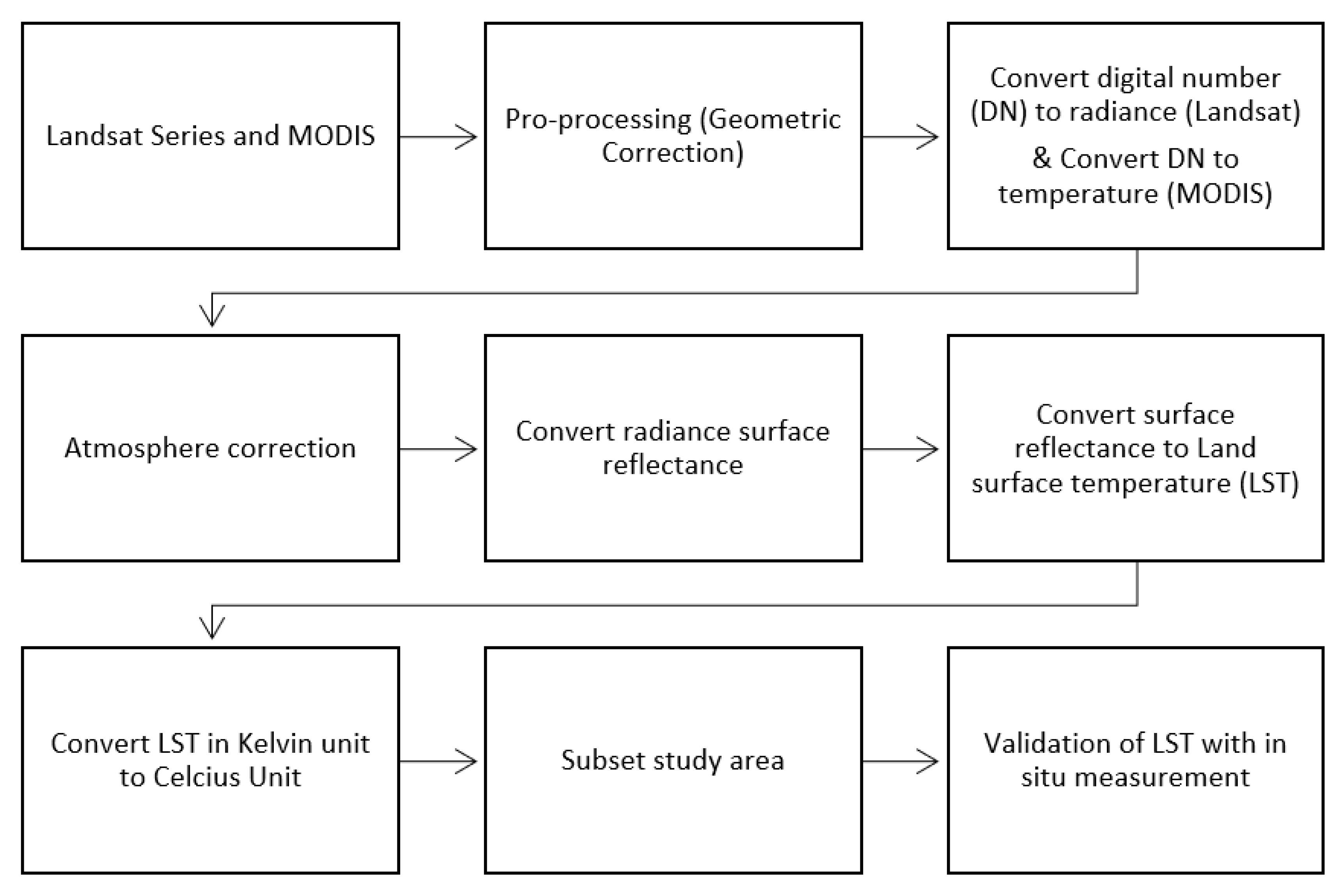
In addition to RS data, daily air temperature data from the Kuching Airport station were collected. The temperature measurements were recorded at latitude 01°29′ north and longitude 110°20′ east. The data, provided in °C, included minimum, maximum, and average monthly temperature values calculated from daily measurements. The meteorological data from the Malaysia Meteorology Department (MMD) covered the period from 1988 to 2019. These data served as a reference to evaluate the accuracy and effectiveness of RS data in studying the impact of ENSO on the temperature in Kuching City, Sarawak. The RS data required preprocessing, including geometric, radiometric, and atmospheric corrections, before converting the digital numbers to land surface temperature, as mentioned in Figure 2. The conversion process follows the method applied by Kemarau and Eboy [22].

Temporal or long-term geometric correction is important for accurately and effectively studying changes in remote sensing data analysis. This study utilizes a polynomial method to obtain low- and simple-resolution satellite image geometry. The relationship between image coordinates (X′, Y′) and cartography (X, Y) is defined by the following:

$${\mathrm{X}}^{\prime }={\mathrm{P}}_{\mathrm{I}}^{\mathrm{N}}\left(\mathrm{X},\mathrm{Y}\right){\mathrm{Y}}^{\prime }={\mathrm{P}}_2^{\mathrm{N}}\left(\mathrm{X},\mathrm{Y}\right){\mathrm{X}}^{\prime }$$

The polynomial ${\mathrm{P}}_{\mathrm{I}}^{\mathrm{N}}$ (where N is the order) is represented by the following:

$${\mathrm{P}}_{\mathrm{I}}^{\mathrm{N}}\left(\mathrm{X},\mathrm{Y}\right)={\displaystyle \sum }_{\mathrm{j}=0}^{{\mathrm{m}}_1}{\displaystyle \sum }_{\mathrm{k}=0}^{{\mathrm{m}}_2}{\mathrm{a}}_{\mathrm{jk}}{\mathrm{X}}^{\mathrm{j}}{\mathrm{Y}}^{\mathrm{k}}$$

with 0 ≤ m_i ≤ n_i, ≤ n, m₁ + m₂ ≤ n.

To determine the accuracy of polynomial geometric correction in Equation (1), ground control points (GCPs) for surface temperature within the image (X′, Y′) need to be selected accurately on the map (X, Y). The minimum number of GCPs depends on the polynomial order through the equation (n + 1) × (n + 2)/2, where n represents the polynomial degree. A large number of GCPs are used to achieve optimal conversion with the smallest overall positional error at the selected points [23].

Atmospheric correction for thermal channels aims to reduce and remove the atmospheric effects from thermal infrared data. The in-scene atmospheric correction (ISAC) algorithm, as proposed by Young et al. [24], is used in this study. ISAC utilizes radiance data at the aperture to estimate the atmospheric radiance and transmission according to Equation (3), employing Equation (1) for the total radiance at the aperture and assuming objects with the highest radiance are either black or blackbody emissive.

Lob = τB(T) + Lu

where Lob is the observed radiance at the aperture, τ represents atmospheric transmission, B(T) denotes the Planck function, and Lu represents the radiance due to the atmosphere. ISAC estimates the surface radiance from the brightness temperature of each pixel.

For each spectral channel, a scatter plot is constructed based on the Planck formula. A straight line is fitted to the upper part of the scatter plot, where pixels approach an emissivity value of 1.0. Subsequently, the estimation of transmission (slope) and upwelling (intercept) is performed. The terms transmission and upwelling are used to approximate the surface radiance leaving the Earth’s surface for each pixel in the original cube. The plotting of transmission and upwelling (τ, Lu) and the generation of the cube are input into the ENVI 5.3 algorithm to implement thermal atmospheric correction through ISAC.

In this study, ENVI 5.3 software is utilized for data pre-processing, including atmospheric correction and conversion of digital numbers to surface temperature. Atmospheric correction plays a vital role in mitigating and removing atmospheric effects on thermal infrared data. The thermal bands in Landsat 4 and 5 TM are located in Band 6. Initially, the sensor captures radiance values in digital numbers, which are then processed using calculations based on previous studies [25], such as Equation (1) below:

$${\mathrm{L}}_{\mathsf{\lambda }}=\left(\frac{{\mathrm{LMAX}}_{\mathsf{\lambda }}-{\mathrm{LMIN}}_{\mathsf{\lambda }}}{{\mathrm{Q}}_{\mathrm{calmax}}-{\mathrm{Q}}_{\mathrm{calmin}}}\right)-\left({\mathrm{Q}}_{\mathrm{cal}}-{\mathrm{Q}}_{\mathrm{calmin}}\right)+\left({\mathrm{LMIN}}_{\mathsf{\lambda }}\right)$$

(1)

As per Equation (1), the variables are defined as follows: L_λ represents the pixel value as radiance in W/(m² × sr × μm), LMAX_λ is the spectral radiance scale factor to Q_calmax in W/(m² × sr × μm), and LMIN_λ is the spectral radiance scale factor to Q_calmin in W/(m² × sr × μm). Q_calmax corresponds to the maximum calibrated pixel value (equivalent to LMAX) in DN, which is 255, while Q_calmin corresponds to the minimum calibrated pixel value (equivalent to LMIN) in DN.

The information regarding LMAX and LMIN was obtained from the downloaded metadata accompanying the remote sensing (RS) data (

Table 2. LMAX and LMIN information for Landsat 5 TM.

Information	Value
${\mathrm{LMAX}}_{\mathsf{\lambda }}$	15.303
${\mathrm{LMIN}}_{\mathsf{\lambda }}$	1.238

). In the case of Landsat 8 OLI TIRS, surface radiance in the thermal spectrum is captured by the Thermal Infrared Sensor (TIRS) 10. To convert digital numbers to radiance spectra L_λ above the atmosphere, Equation (2) is applied as follows:

$${\mathrm{L}}_{\mathsf{\lambda }}=\mathrm{ML}\times \mathrm{Qcal}+{\mathrm{A}}_{\mathrm{L}}$$

(2)

In this study, the radiance spectrum L_λ is measured in units of W/(m²·sr·μm), while ML represents the recalibrated gain for a specific band, also in units of W/(m²·sr·μm). A_L corresponds to the path radiance, measured in units of W/(m²·sr·μm). The ENVI 5.3 software is employed, which provides thermal functions specifically designed for atmospheric correction purposes. Before conducting atmospheric correction, it is necessary to convert the thermal images into radiance format.

The primary objective of atmospheric correction for thermal bands is to minimize and remove the atmospheric effects present in thermal infrared data. This study utilizes the in-scene atmospheric correction (ISAC) algorithm proposed by Young et al. [22]. ISAC relies on radiance data acquired at the aperture to estimate the upwelling radiance and atmospheric transmission, as described in Equation (3). Furthermore, Equation (1) is employed to calculate the radiance at the aperture, assuming that objects with the highest radiance are black.

Lob = τB(T) + Lu

(3)

The term “radiance” refers to the observed radiance at the aperture, while τ represents the atmospheric transmission. B(T) corresponds to the Planck function, and Lu represents the upwelling radiance due to the atmosphere. The in-scene atmospheric correction (ISAC) algorithm evaluates the surface radiance emitted based on the brightness temperature of each pixel. The scatter plot of radiance for each band follows the Planck formula. A linear regression line is fitted to the upper portion of the scatter plot, which represents pixels approaching an emissivity of 1.0. This process estimates the transmission (slope) and upwelling (intercept) factors. These factors, referred to as “transmission” and “upwelling”, approximate the surface radiance leaving the Earth for each pixel within the original cube. By plotting the transmission and upwelling (τ, Lu) and generating the cube, the ENVI 5.3 algorithm incorporates this information to perform thermal atmospheric correction using ISAC.

In the case of Landsat 5 TM, information regarding the sensor is stored in the Landsat 5 TM metadata file. Assuming the Earth’s surface behaves as a blackbody emitter with a spectral radiance, the radiance spectrum obtained from the sensor is then converted into an effective sensor brightness temperature using Equation (4) [25].

$${\mathrm{T}}_{\mathrm{B}}=\frac{{\mathrm{k}}_2}{\ln \left(\frac{{\mathrm{k}}_1}{{\mathrm{L}}_{\mathsf{\lambda }}}+1\right)}$$

(4)

In Equation (4), T_B represents the effective sensor brightness temperature in Kelvin (K), while ${\mathrm{k}}_1$ and ${\mathrm{k}}_2$ are calibration constants. For Landsat 5 TM, the values for ${\mathrm{k}}_1$ and ${\mathrm{k}}_2$ are set to 607.76 K and 1260.56 K, respectively. It is important to note that the sensor brightness temperature obtained from Equation (4) is related to a black body. To estimate the surface temperature of a gray body, the emissivity of the surface spectrum needs to be improved. This can be achieved by calculating the improved surface temperature emissivity using Equation (5) proposed by Artis and Carnahan [26].

$$\mathrm{LST}=\frac{{\mathrm{T}}_{\mathrm{B}}}{1+\left({\mathsf{\lambda }\mathrm{T}}_{\mathrm{B}}∕\mathsf{\alpha }\right)\mathrm{In}\mathsf{\epsilon }}$$

(5)

The surface temperature is typically measured in Kelvin (K). In the context of the equation mentioned above, T_B represents the effective sensor brightness temperature in K. The variable λ denotes the wavelength of the emitted light, expressed in meters. For the Landsat 5 TM thermal bands, the effective wavelengths are 11.457 μm, 11.269 μm, and 10.904 μm, based on Equation (6) with α = 1.438 × 10⁻² mk. The symbol ε represents the surface emissivity.

To convert the surface temperature from Kelvin to degrees Celsius (°C), Equation (6) is applied as follows:

Surface temperature (°C) = Surface temperature (K) − 273.15

(6)

The thermal surface radiance is captured by the thermal infrared sensor (TIRS) band 10 on Landsat 8 OLI. To eliminate atmospheric effects from the thermal data, preprocessing is conducted. The surface temperature is then derived using the algorithm proposed by He et al. [27].

To convert the digital numbers (DN) to spectral radiance L above the atmosphere, Equation (7) is applied as follows:

L_λ = ML × Qcal + A_L

(7)

In Equation (8), L_λ represents the spectral radiance in units of W/(m·sr·μm)². ML corresponds to the rescaled gain specific to a particular band, measured in units of W/(m·sr·μm)². A_L accounts for the band-specific rescaling bias, also measured in units of W/(m·sr·μm)². It is important to note that the rescaling bias is applied to a specific band.

To extract the sensor brightness temperature Tb in Kelvin (K) from TIRS band 10, similar to the OLI sensor, Equation (8) is utilized as follows:

T_b = K₂/(ln(K₁/L_λ) + 1

(8)

In Equation (9), K₁ and K₂ are predefined constants set to 774.89 (in W/(m·sr·μm)²) and 1321.08 (in W), respectively. The surface temperature is determined by correcting the emitted radiance of the ground (B) in Kelvin (K) using the mono-window algorithm proposed by Qin et al. [28].

NDVI (Normalized Difference Vegetation Index) is calculated using Equation (9), where ρNIR and ρRED represent the values of the near-infrared and red bands, respectively. Calculating NDVI is important as it closely relates to the vegetation cover fraction (Pv). Pv represents the percentage of vegetation in the pixel and is calculated based on Carlson and Ripley [29] using Equation (9):

Pv = ((NDVI − NDVIs)/(NDVIv − NDVIs))²

(9)

Pv is also related to the emissivity (E), which is calculated using Equation (10):

Ε = εv Pv + εg (1 − P) + 4 <dε> Pv (1 − Pv)

(10)

In Equation (10), ε represents the land emissivity, εv represents the emissivity of pure vegetation (set to 0.985), εg represents the emissivity of bare soil (set to 0.960), and <dε> is a parameter adjusted to an average of 0.01.

Finally, the surface temperature in Kelvin is converted to Celsius using Equation (11):

Surface temperature = (TB/(1 + (λ × TB/C2) × ln(ε))) − 273.15

(11)

In Equation (11), TB represents the sensor brightness temperature in Kelvin (K), ρ = hc/σ, where σ is the Boltzmann constant (1.38 × 10⁻²³ J/K), h is the Planck constant (6.626 × 10⁻³⁴ J/s), c is the speed of light (2.998 × 10⁸ m/s), and ε is the emissivity.

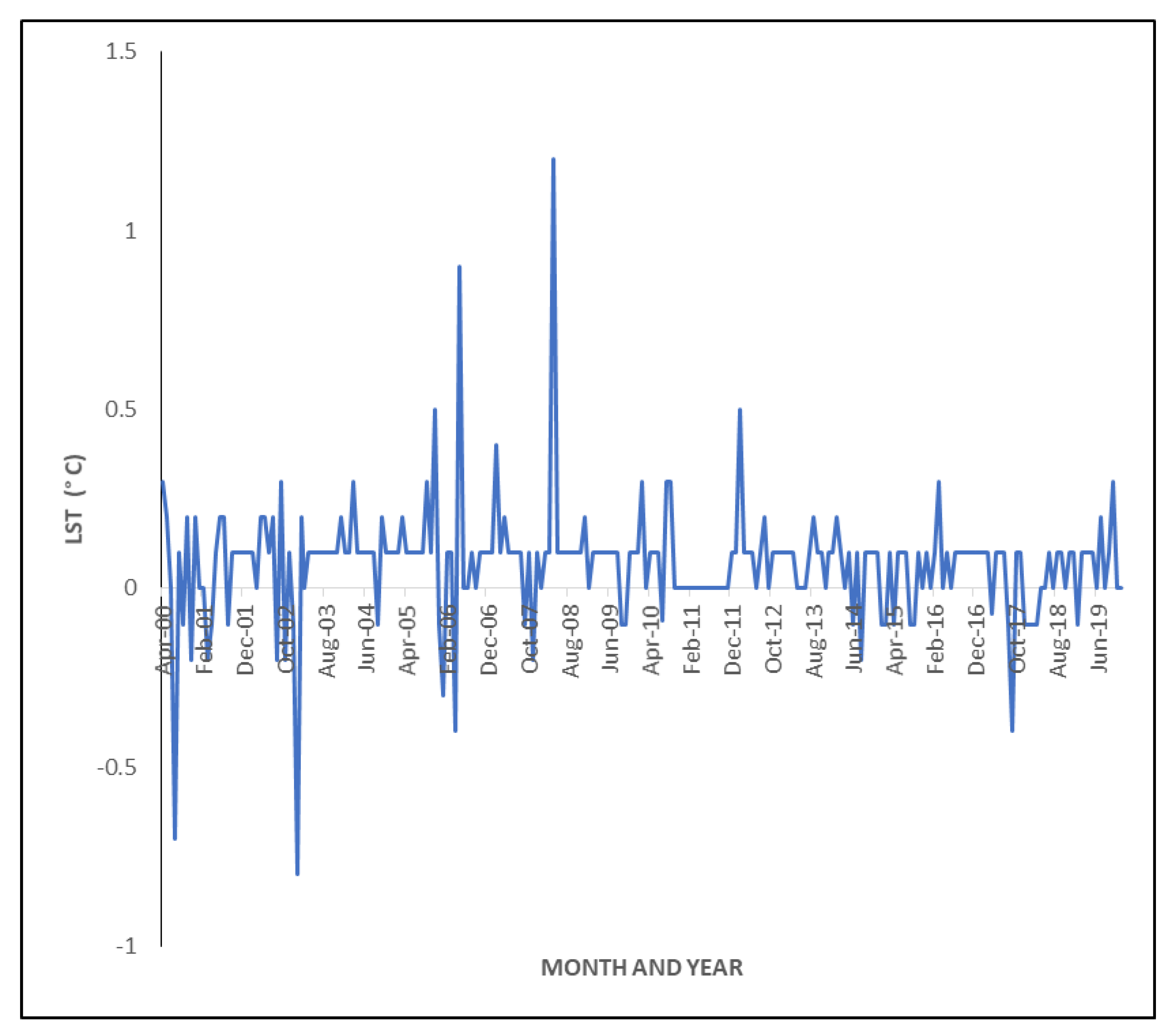
Overall, the temperature differences between MODIS satellite data and MMD data are lower compared to the differences between Landsat satellite data and MMD data. For example, MODIS satellite data have the largest temperature difference of +1.2 °C compared to that of the MMD data, while Landsat data has a difference of −1.7 °C (Figure 3). The 0.5 °C difference between the two RS datasets is due to the characteristics of the data. MODIS represents the monthly average temperature, while Landsat represents the daily average temperature. Daily average temperature data has higher variability due to daily weather fluctuations compared to monthly average temperature, which represents the overall average of daily temperatures [4].

The selection of RS data depends on the research objectives of the investigators. Previous studies have reported that MODIS data are highly suitable for studies involving regional and global scales due to their 5600 m resolution. Additionally, researchers can gain a detailed understanding of land surface temperature changes because MODIS data are obtained from two satellites, Aqua and Terra, which provide daily data both during the day and at night. MODIS data can be obtained in various time scales, including daily, 8-day average, weekly average, monthly average, and annual average temperatures. The continuous and freely available data provided to researchers worldwide have made MODIS data the second most important dataset for studying weather and climate changes, especially temperature data.

However, MODIS data were launched in 1999, and the data were usable from 2000 onwards. This means that researchers lost useful data before 2000. This is why the Landsat satellite is the preferred choice for studying temperature, as the Landsat series, including Landsat 4/5 TM, 7 ETM, 8 OLI TIRS, and 9 OLI TIRS 2, has been providing data from 1989 to 2021. This has allowed researchers to extensively study the impact of development changes on temperature [5,6]. Furthermore, Landsat data offer the highest thermal data resolution for temperature studies, currently at 100 m, compared to the 5600 m resolution of MODIS. With this moderate resolution advantage of 100 m, thermal data play a crucial role in studying the effects of land use and land cover on temperature.

3. Results

This section is divided into three sub-sections, the first and second of which detail the relationship between the LST from Landsat and MODIS, and monthly temperature of the Malaysia Meteorology Department. The third subsection is on the distribution of LST Landsat and MODIS data during ENSO.

3.1. Relationship between ONI with LST Landsat, LST MODIS, and Monthly Temperature of the Malaysia Meteorology Department

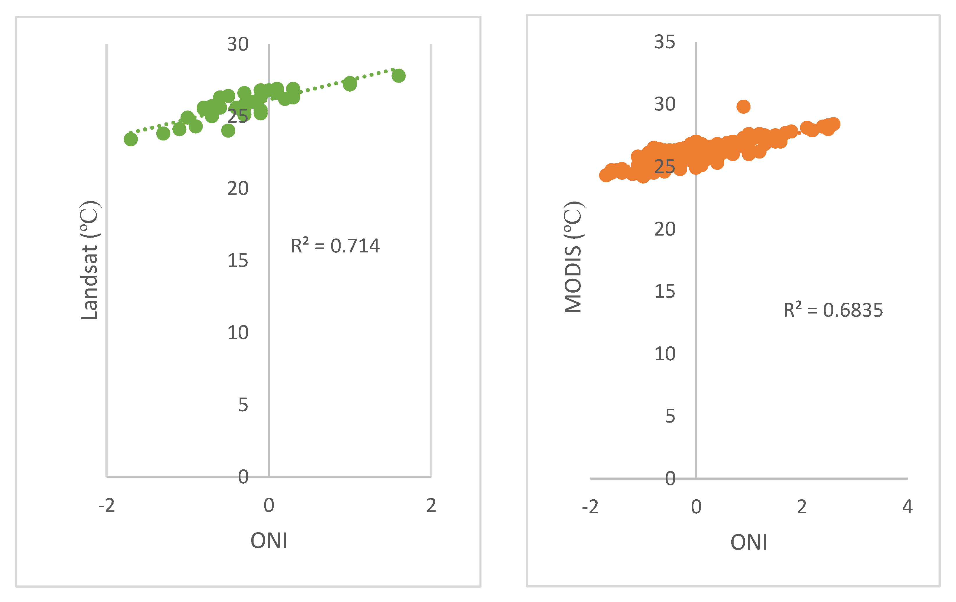
The correlation coefficient (R²) between the ONI and Landsat is 0.71, which is slightly higher than the correlation of 0.68 between the ONI and MODIS surface temperature (Figure 4). However, both correlations indicate a significant relationship between the ONI and the temperature data obtained from both satellite sources. The R² values exceeding 0.50 suggest that changes in the ONI correspond to temperature variations captured by both the MODIS and Landsat satellites.

The higher R² value between the temperatures from the ONI and MODIS satellites compared to that of the Landsat satellites can be attributed to the larger amount of MODIS data available, allowing for a more accurate representation of both variables [5]. The correlation graph in Figure 4 visually demonstrates the positive relationship between the ONI and surface temperature for both the MODIS and Landsat satellites. This indicates that an increase in the ONI is associated with higher surface temperatures recorded by both satellite systems. These findings provide evidence that ENSO, as indicated by the ONI parameters, influences the surface temperature captured by both the MODIS and Landsat satellites. This study utilizes a correlation analysis to accomplish our fourth objective.

The validation of data resulting from satellite remote sensing and ground observations is crucial to assess the accuracy and reliability of the remote sensing data in studying the impact of El Niño–Southern Oscillation (ENSO) on the temperature in Kuching City, Sarawak. The purpose of the correlation analysis is to establish a benchmark and evaluate the effectiveness of remote sensing (RS) data in this context.

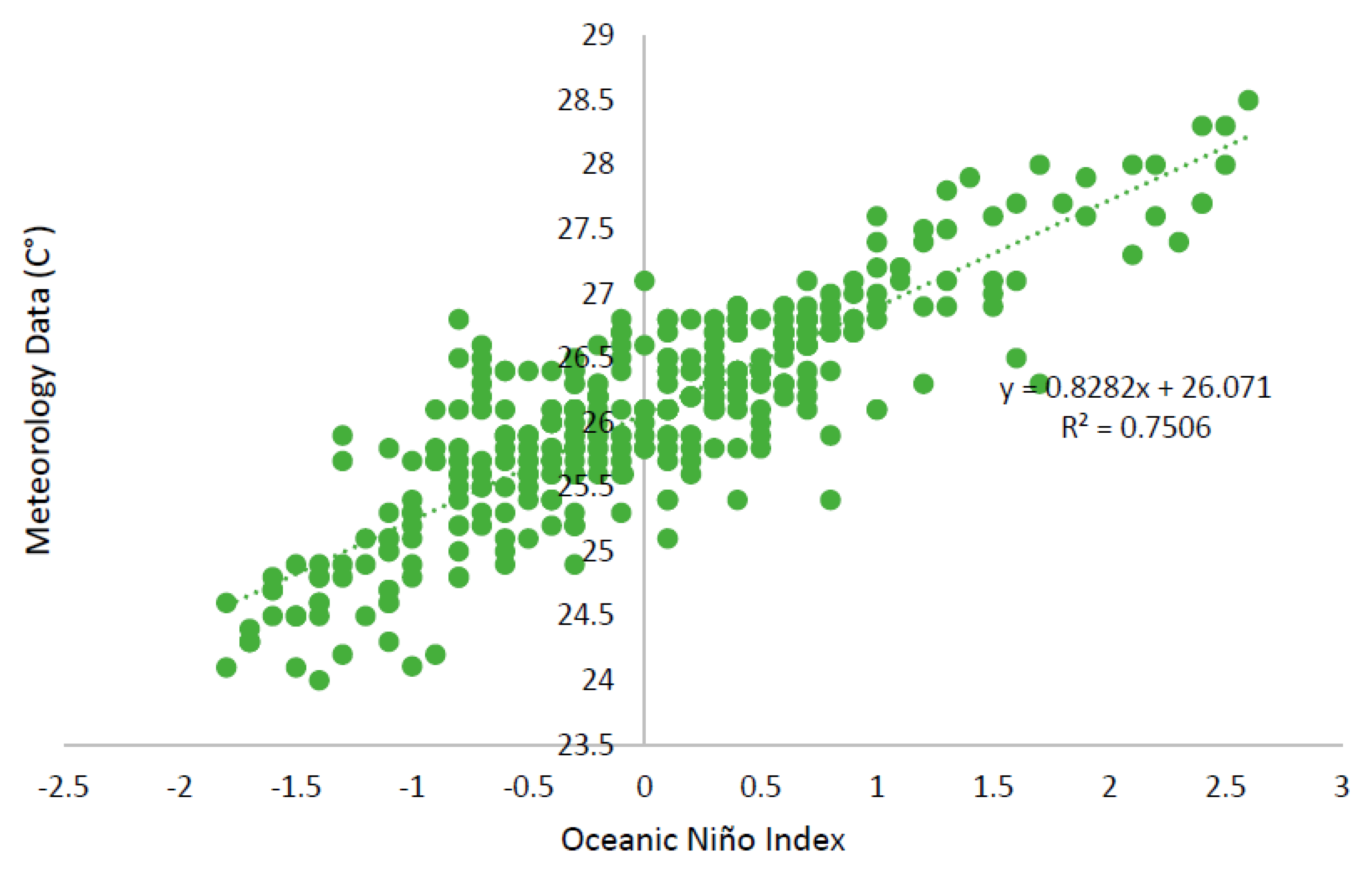
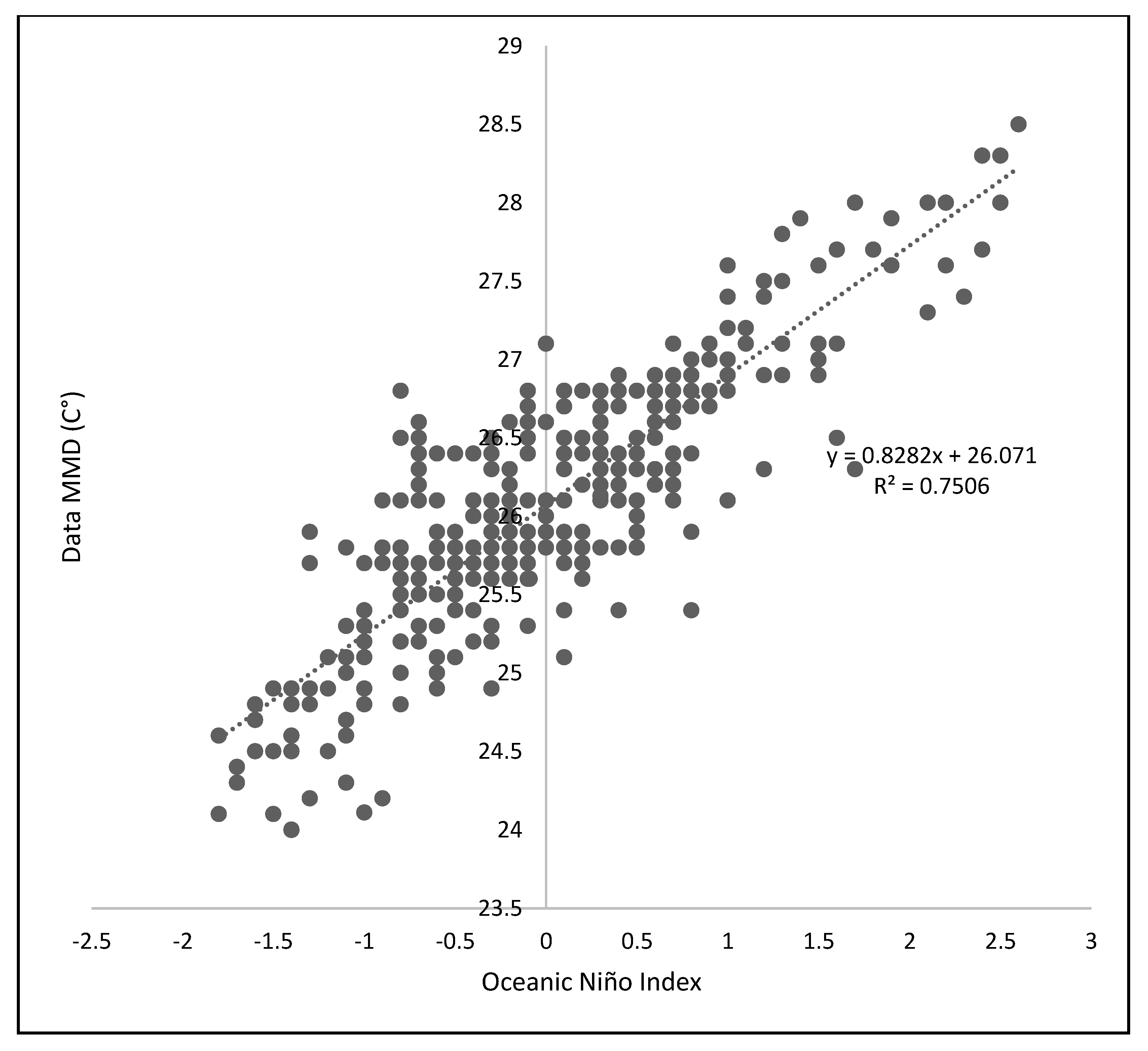
The correlation between the Oceanic Niño Index (ONI), which serves as an indicator of ENSO, and the air temperature for three months is shown in Figure 4. The analysis utilizes 385 monthly average temperature data from the Malaysian Meteorological Department (MMD) and corresponding ONI values from 1988 to 2019. Our expectation is to observe a positive relationship between the RS temperature and the ONI, with a correlation coefficient (R²) exceeding 0.5 (R² > 0.5). The results presented in Figure 4 demonstrate a strong positive correlation between the ONI and air temperature from the MMD, with an R² value of 0.75. This finding indicates that the occurrence of ENSO, as indicated by the ONI, directly influences the air temperature in Kuching City. Specifically, an increase in the ONI is associated with a rise in air temperature, while a decrease in the ONI corresponds to a decrease in air temperature.

It is important to note that an ONI value exceeding one signifies the presence of El Niño, which is often accompanied by elevated temperatures and the onset of drought conditions. Therefore, the higher-than-usual temperatures observed in Kuching City, Sarawak, can be attributed to the occurrence of El Niño events. By validating the correlation between the RS temperature and the ONI, this analysis confirms the impact of ENSO on the air temperature in the study area. These findings enhance our understanding of the relationship between ENSO and temperature dynamics, providing valuable insights for climate studies, environmental monitoring, and informing measures to mitigate the impact of El Niño events in Kuching City, Sarawak.

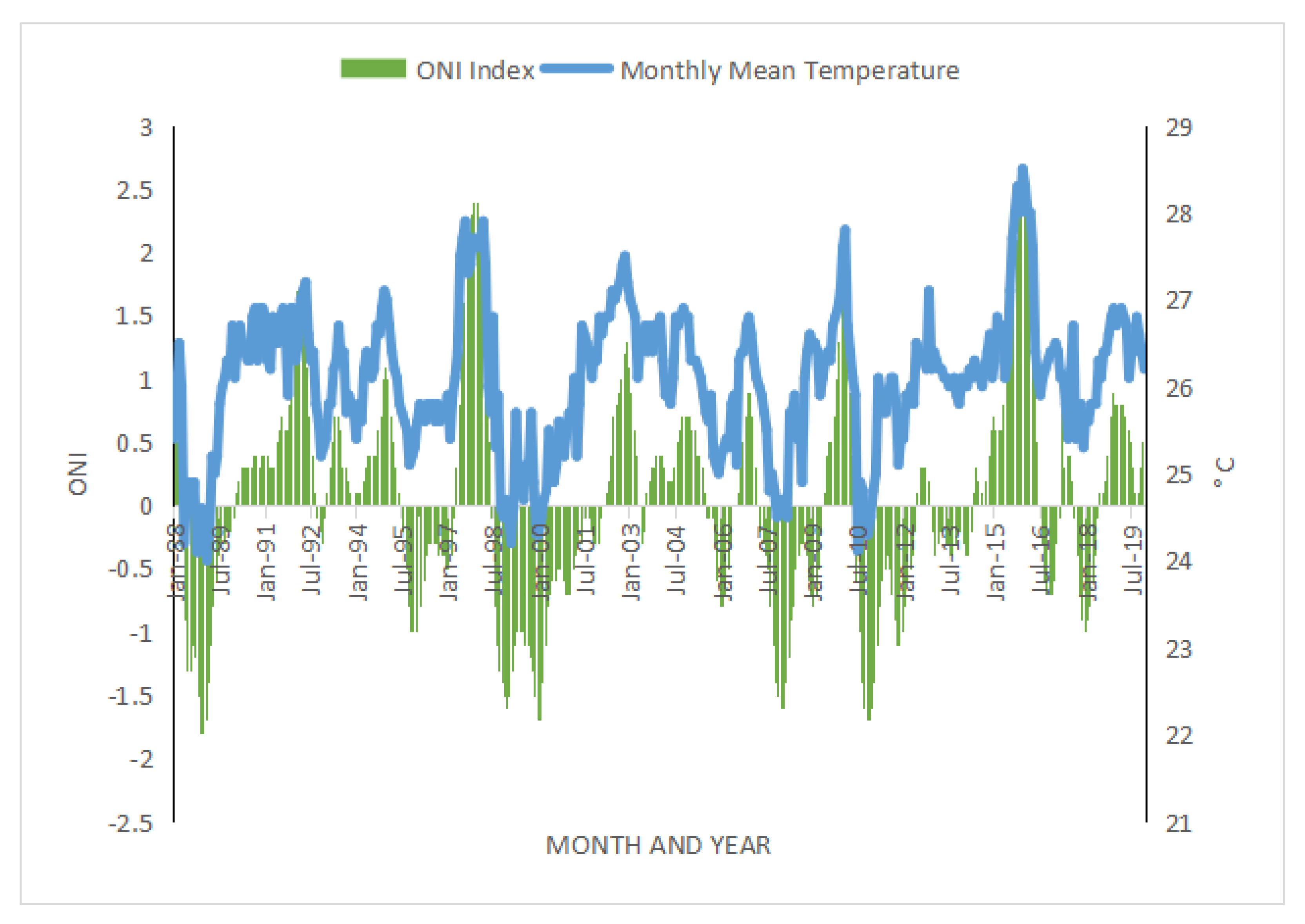
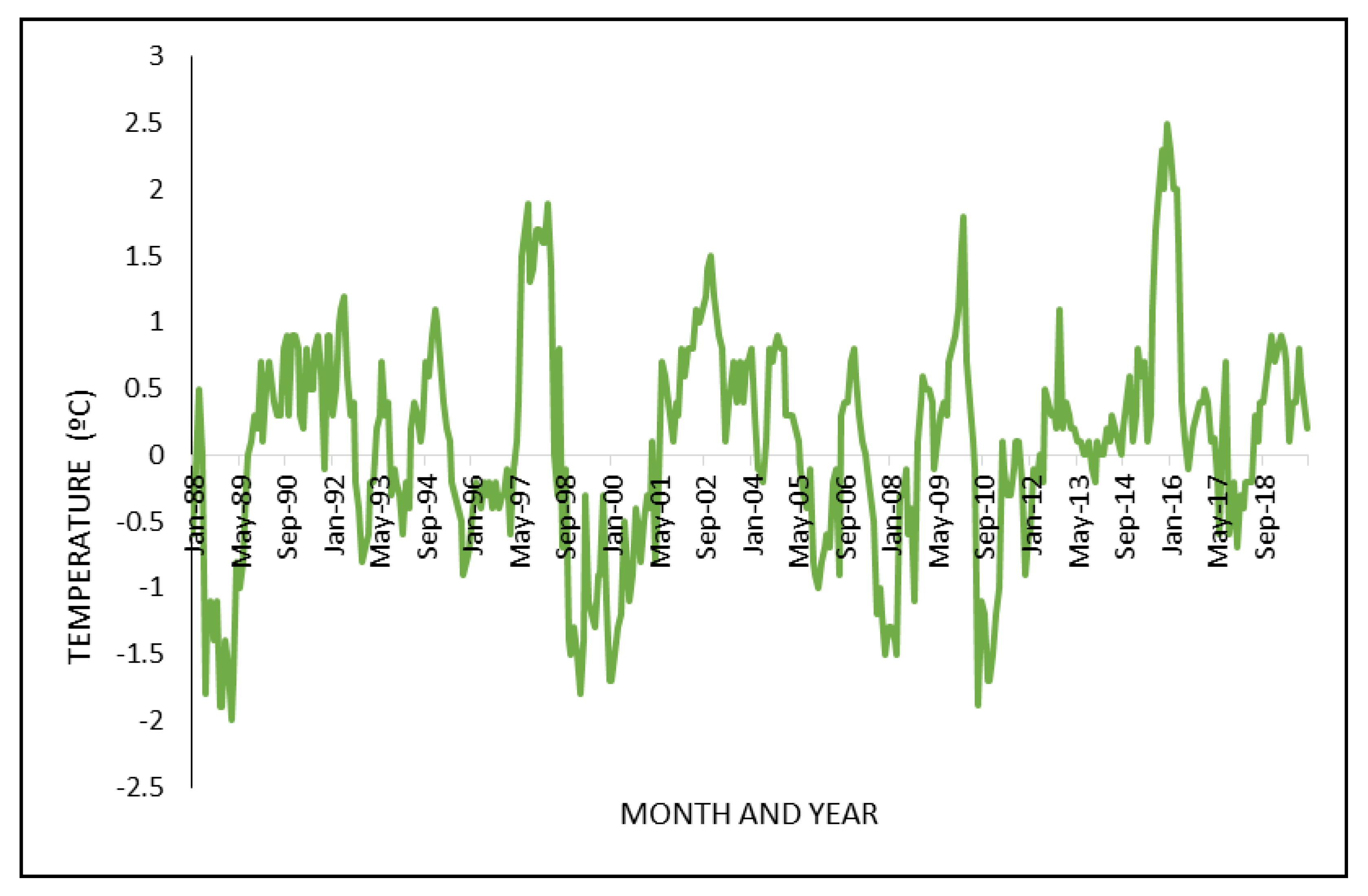
The temporal pattern of the ONI and air temperature, representing the average monthly temperature in Kuching City from 1988 to 2019, is shown in Figure 5. As depicted in Figure 6, a positive relationship between the ONI and monthly temperature from MMD is observed. From May 1988 to May 1989, the ONI values ranged from −1 to −1.8, resulting in a decrease in temperature from 24.8 °C to 24 °C. Negative ONI values indicate the occurrence of La Niña events, observed in December 1999, 2007, and 2010. In contrast, during El Niño events spanning from June 1997 to April 1998, the recorded ONI was 0.88, leading to an increase in temperature from 26.48 °C to 27.9 °C. A similar phenomenon recurred from late 2015 to March 2016. El Niño events also occurred in 1991, 1997–1998, and 2015–2016 [13,14,15].

To further understand the relationship between independent and dependent variables, this study employs a linear regression model. This model helps elucidate changes in the dependent variable using an independent variable. According to De Sá [30], the linear regression model is regarded as the most stable approach in scientific research.

Table 3. Results of the linear regression analysis of the impact of ENSO on air temperature obtained from the MMD in Kuching City, Sarawak.

Model	R	R2	Adjusted R2	The Standard Error for the Estimation
1	0.866	0.75	0.75	0.40861

presents the results of the linear regression analysis, aiming to comprehend the impact of ENSO on the air temperature obtained from the Meteorological Department in Kuching City, Sarawak.

(a)

Predictors: (Constant) ONI Index

Table 3 reports the coefficients of R and R². An R-value of 0.866 indicates a high correlation, indicating a significant relationship between the ONI and air temperature from the MMD. Moreover, an R² value of 0.75, which indicates the extent to which the total variation in the dependent variable (temperature from the MMD) can be explained by the independent variable (ONI), indicates that 75% of the temperature can be explained by the ONI.

Table 4. ANOVA for the effect of ENSO occurrence on temperature from MMD.

Model	Sum of Squares	Df	Mean Square	F	Sig
Regression	191.949	1	191.949 0.163	1149.6	0.00
Residual	63.779	382
Total	255.728	383

below illustrates the extent to which the regression equations correspond to the data to understand the dependent variables.

(a)

Dependent Variable: Monthly mean temperature

(b)

Predictors: (Constant): ONI Index

Table 4 presents the results of the linear regression model, which aims to understand the relationship between the dependent variables. In a regression analysis, the p-value is used to assess the significance of the regression model. If the p-value is less than 0.05 (p < 0.05), it indicates that the regression model corresponds well to the data and is considered statistically significant. In this study, the linear regression model between the ONI parameters and temperature from the MMD yielded a p-value of 0.000. This very low p-value indicates a highly significant relationship between the ONI parameters and MMD temperature data. Therefore, our results support the robustness and reliability of the ONI and temperature data used in the analysis. Overall, our findings suggest that the linear regression model effectively explains the relationship between the ONI parameters and temperature from MMD, providing valuable insights into the impact of ENSO on temperature patterns in the study area.

Table 5. Single regression formula for understanding the effect of ONI on three dependent parameters to predict the effect of ENSO occurrence on air temperature and land surface temperature.

The Dependent Variable (Y)	Model Prediction Impact ONI (X)	Adjusted R2	p Value
Monthly mean temperature MMD	Y = 0.828 × (X) + 26.071	0.75	0.000
LST MODIS	Y = 0.832 × (X) + 26.087	0.68	0.000
LST Landsat	Y = 1.139 × (X) + 26.610	0.55	0.000

shows a single regression formula for understanding the effect of the ONI on three dependent parameters to predict the impact of ENSO occurrences on air temperature and surface temperature. The table presents the adjusted R² values, which indicate the proportion of variation in the dependent variables that can be explained by the ONI. Based on Table 5, the highest adjusted R² value is observed for the monthly average temperature from the MMD, with a coefficient of 0.75. The second highest value is for the surface temperature from the MODIS satellite, with a coefficient of 0.68, followed by the surface temperature from the Landsat satellite, which has an adjusted R² value of 0.55.

The higher adjusted R² coefficient for the monthly average temperature from the MMD (0.75) can be attributed to the larger amount of data available for this parameter (386 data points), compared to 238 MODIS data points and 37 Landsat data points. The number of data points plays a significant role in determining the adjusted R² value. However, it is important to note that the adjusted R² for the surface temperature of the MODIS satellite is 0.68, and for the Landsat satellite, it is 0.55. Although the adjusted R² values differ among the variables, all three regression models are considered reliable as they exceed the threshold of 0.50 or 50% [31]. This means that 50% of the variation in the air temperature from the MMD, the surface temperature from MODIS, and the surface temperature from Landsat satellites can be explained by the ONI.

The positive relationship between the ONI and the dependent variables is demonstrated by the adjusted R² values. This indicates that an increase in the ONI is associated with an increase in parameters such as the air temperature from the MMD, the surface temperature from the MODIS satellite, and the surface temperature from the Landsat satellite. Thus, 50% of the variation in these variables can be explained by the ONI. In summary, the adjusted R² values in Table 5 illustrate a positive relationship between the ONI and the monthly average temperature from the MMD, as well as the surface temperature from the MODIS and Landsat satellites. This implies that an increase in the ONI corresponds to higher values for the mentioned parameters.

3.2. Land Surface Temperature Distribution during El Niño and La Niña in Kuching City from Landsat

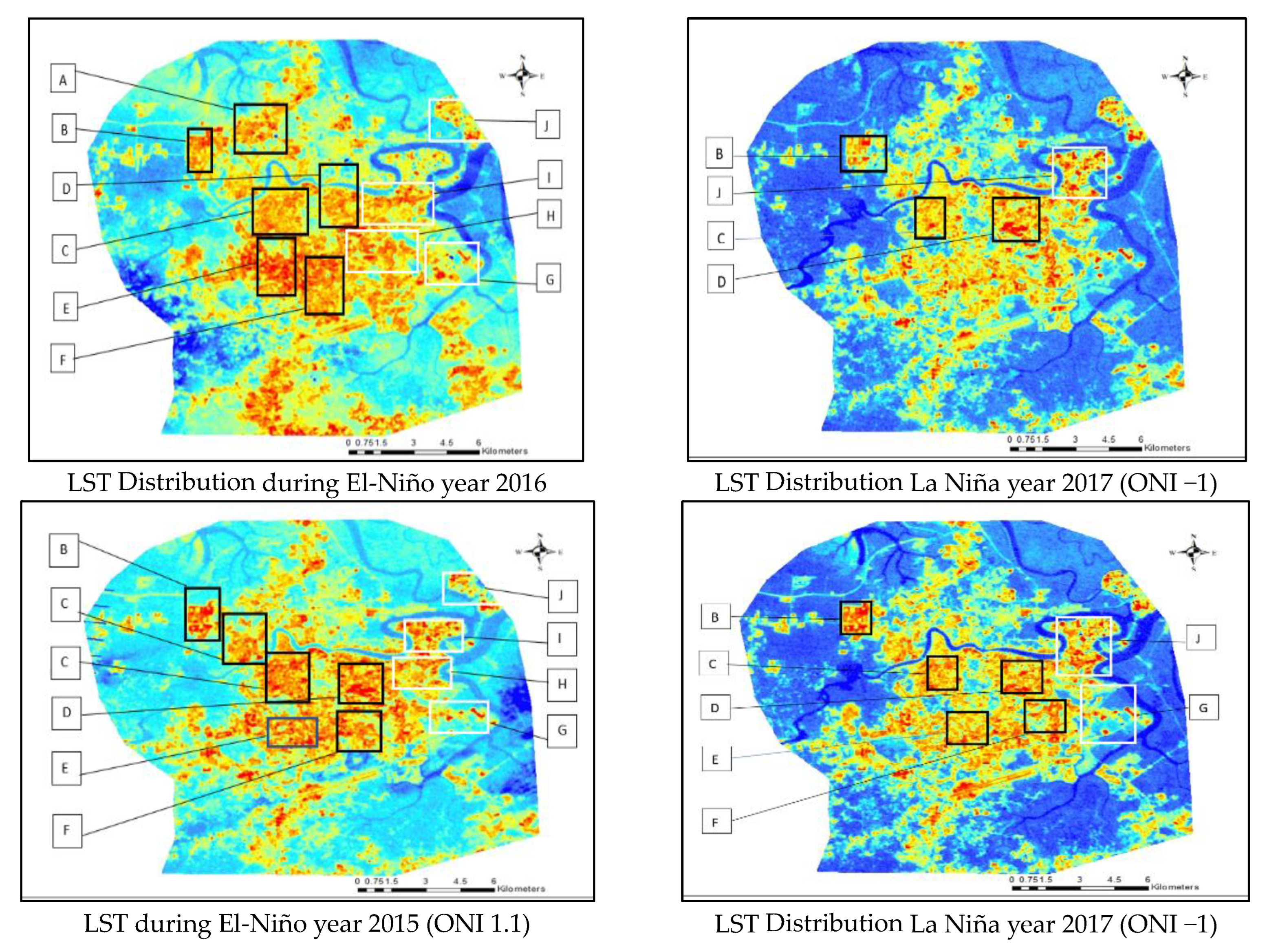
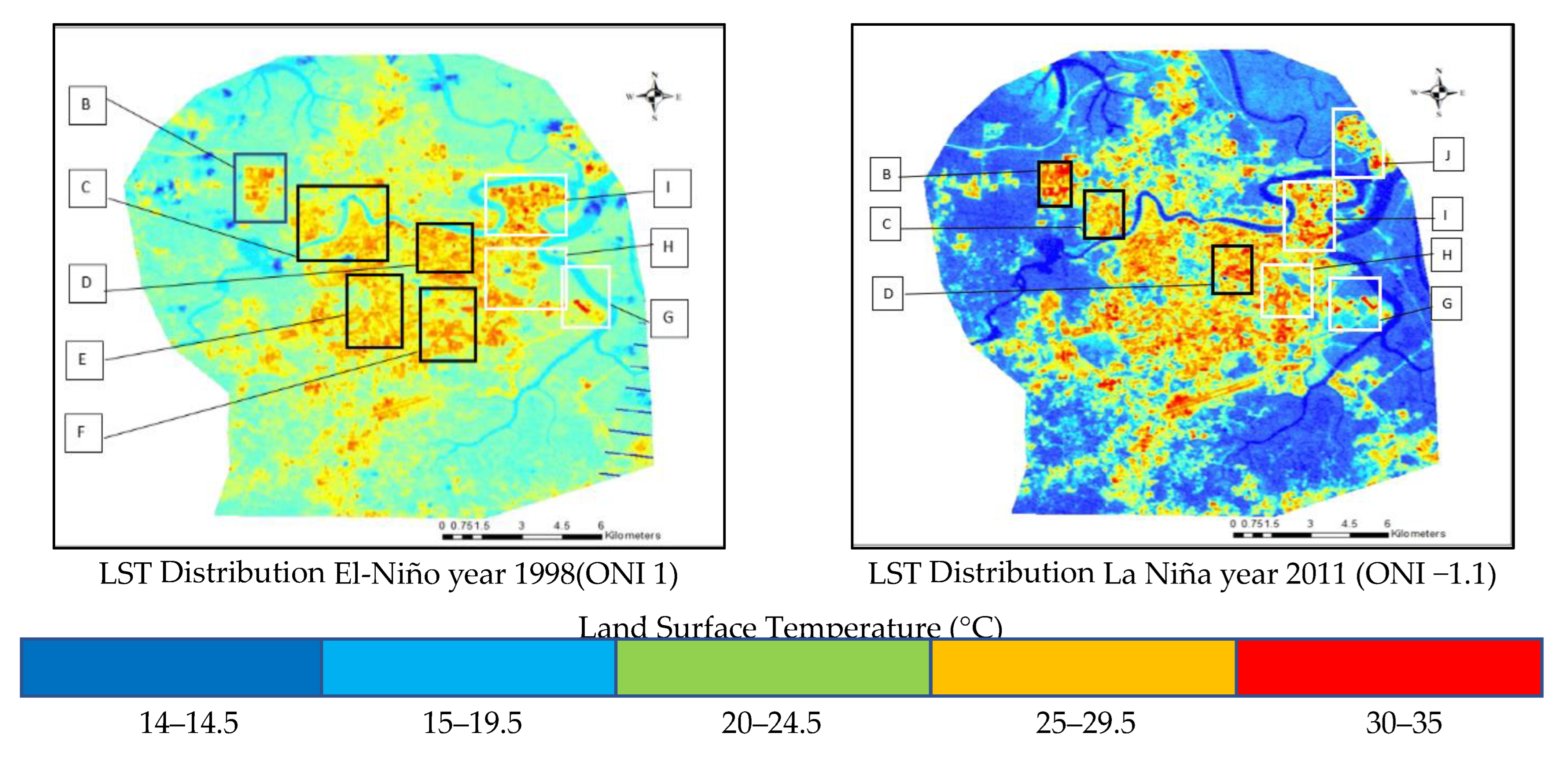
Based on Figure 7, the left side depicts the dates when the Landsat data were recorded during the El Niño event, with ONI values of 1 to 1.1. On the other hand, the right side of Figure 5 displays maps of the temperature distribution during La Niña, with negative ONI values ranging from −1 to −1.1. The temperature distribution map during El Niño illustrates that most study locations in Kuching City, Sarawak, are colored in shades of yellow, indicating higher-than-normal surface temperatures. Conversely, during the La Niña event, the temperature map shows bluish shades, representing lower local temperatures compared to the El Niño event.

To gain a clearer understanding of the areas experiencing higher temperatures, the study categorizes them into urban and industrial zones. In Kuching City, Sarawak, there are more clustered heat areas during El Niño compared to La Niña. For instance, during El Niño, almost all of the zones (B, C, D, E, F, G, H, I, and J) exhibit temperatures above 30 °C [31], causing discomfort to the population in Kuching City, as shown in Figure 8. Another example is illustrated in Figure 6. During El Niño, there are a total of eight focal point hot zones: B, C, D, E, and F (urban areas) and G, H, and I (industrial areas), while during La Niña, there are seven zones: B, C, D, G, H, I, and J. Figure 5, Figure 6 and Figure 7 demonstrate the increase in the area of concentrated heat where the temperatures exceed 30 °C, during both La Niña and El Niño events.

To further understand the impact of ENSO events on temperature distribution using remote sensing techniques in Kuching City, Sarawak, this study analyzes the statistical values of the maximum, minimum, and average temperatures derived from Landsat satellite data during La Niña and El Niño events.

Table 6. Information on the statistical values of maximum, minimum, and mean LST Landsat during ENSO events in Kuching City.

Date	ONI Value	Statistic Value LST (°C)	Date	ONI Value	Statistic Value LST (°C)	LST Difference (°C)
24 October 2018	−1 (La Niña)	Maximum (31.39)	6 July 2016	1 (El-Niño)	Maximum (35.90)	Maximum (4.51)
		Minimum (19.10)			Minimum (24.29)	Minimum (5.29)
		Mean (24.8)			Mean (26.90)	Mean (2.10)
21 August 2018	−1 (La Niña)	Maximum (31.71)	28 July 2015	1.1 (El-Niño)	Maximum (34.33)	Maximum (2.62)
		Minimum (23.45)			Minimum (25.19)	Minimum (2.74)
		Mean (24.2)			Mean (26.72)	Mean (2.52)
9 November 2011	−1.1 (La Niña)	Maximum (30.55)	3 April 1998	1 (El-Niño)	Maximum (33.31)	Maximum (2.76)
		Minimum (19.42)			Minimum (26.19)	Minimum (6.77)
		Mean (24.91)			Mean (27.81)	Mean (2.9)

provides comprehensive information on the statistical values of the maximum, minimum, and average temperatures during La Niña and El Niño events in Kuching City. These temperature differences are based on cloud-free Landsat satellite data and ONI values exceeding −1 for La Niña and 1 for El Niño in Kuching City, Sarawak.

The subsequent paragraph delves into a detailed explanation of the variations in the maximum, minimum, and average temperature statistical values derived from Landsat satellite data during La Niña and El Niño events in Kuching City, Sarawak. Table 6 presents statistical information values for the selected data when the ONI exceeds ±1 and there is no cloud coverage at the study location.

In Table 6, it is evident that the average, maximum, and minimum temperatures during El Niño are higher than during La Niña. For instance, during ONI 1.1 in April 1998 (El Niño), the average temperature is 27.81 °C, whereas during ONI −1.1 in November 2011 (La Niña), the average temperature is 24.91 °C. Similar temperature differences can be observed in July 2015, when the average temperature during ONI 1.1 was 26.90 °C (El Niño), which was higher than the average temperature of 24.2 °C during La Niña with an ONI of −1. The same trend applies to the maximum and minimum temperature values. During El Niño, the maximum temperature reached 35.90 °C, and the minimum temperature was 24.29 °C, while during La Niña, the maximum temperature was 31.39 °C, and the minimum temperature was 19.10 °C. These values correspond to ONI 1 in July 2016 (El Niño) and non-October 2017 (La Niña).

Table 6 provides further details on the differences in the maximum, minimum, and average temperatures, showing variances ranging from 2.10 °C to 2.90 °C for the average, 2.32 °C to 4.51 °C for the maximum, and 2.74 °C to 6.77 °C for the minimum values. ENSO events have a significant influence on local temperatures, and RS technology can effectively record and provide information on hot and cold focal spaces during La Niña and El Niño events, as depicted in Figure 7.

Before the advent of RS technology, predicting phenomena such as floods, earthquakes, hurricanes, and droughts was challenging. Researchers worldwide are actively developing specific models to alert the public and enhance preparedness for unexpected events, such as ENSO incidents. By utilizing RS data, the occurrence of natural disasters can be predicted, enabling responsible parties and residents in Kuching, Sarawak, to be better prepared to face events such as droughts and floods, thereby mitigating property damage and the loss of lives.

3.3. Land Surface Temperature Distribution during El Niño and La Niña in Kuching City from MODIS

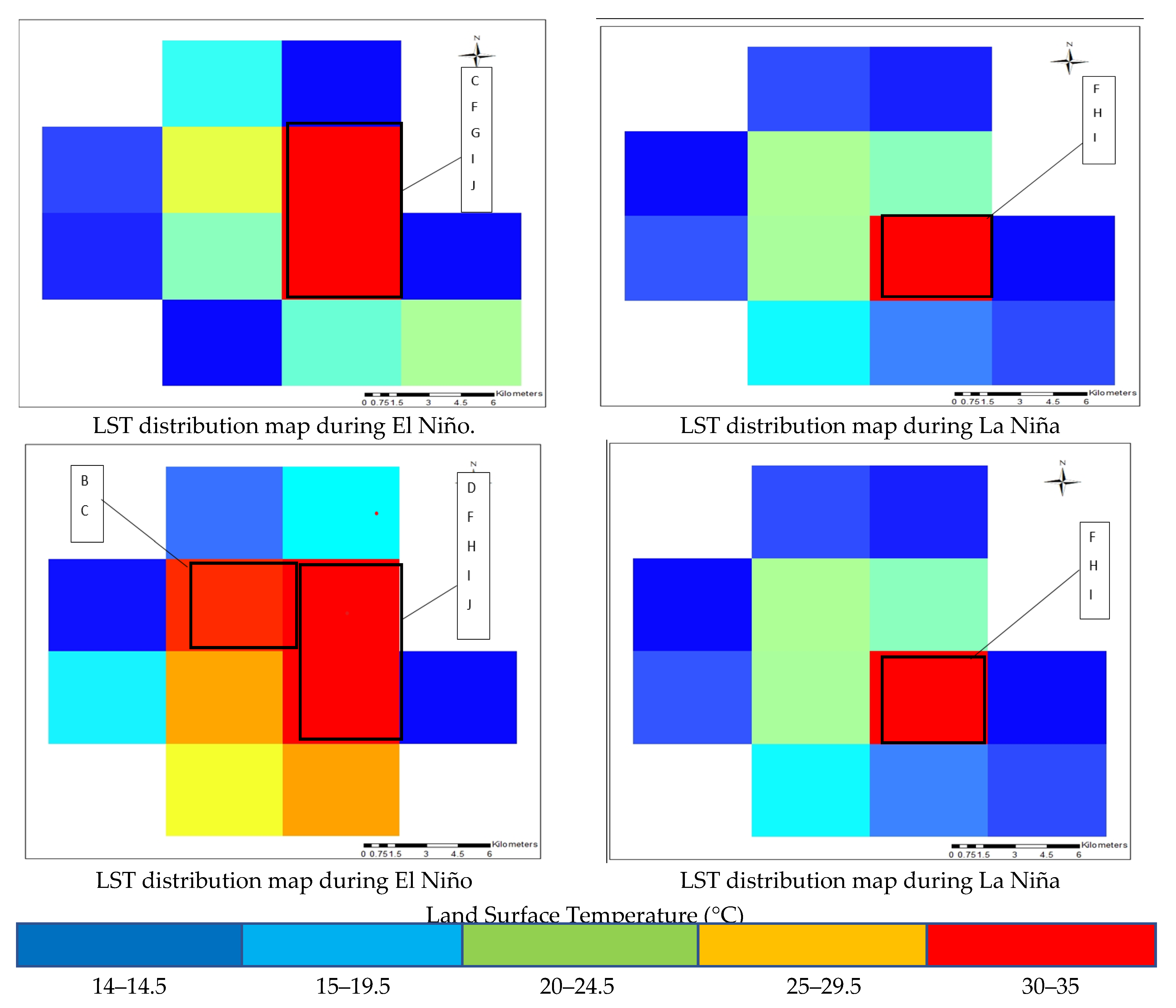
Figure 8 illustrates the pattern of surface temperature distribution in Kuching City, which varies during La Niña and El Niño events. During El Niño, a larger area of extreme land surface temperature is observed compared to that of the La Niña events. For example, during La Niña in January 2010, only one pixel representing zones H and I exceeded a surface temperature of 30 °C. In contrast, during El Niño in January 2016, there were three pixels representing zones B, C, D, F, G, H, I, and J that exceeded the threshold.

Table 7. Information on the statistical values of maximum, minimum, and mean LST MODIS during ENSO events in Kuching City.

Date	ONI Value	Statistic Value LST (°C)	Date	ONI Value	Statistic Value LST (°C)	LST Difference (°C)
December 2010	−1.6 (La Niña)	Maximum (30.05)	February 2016	2.2 (El-Niño)	Maximum (32.11)	Maximum (2.06)
		Minimum (20.87)			Minimum (26.23)	Minimum (5.36)
		Mean (24.5)			Mean (28.01)	Mean (3.51)
November 2010	−1.7 (La Niña)	Maximum (30.71)	January 2016	2.6 (El-Niño)	Maximum (35.31)	Maximum (4.6)
		Minimum (20.51)			Minimum (27.02)	Minimum (6.65)
		Mean (24.3)			Mean (29.01)	Mean (4.71)

presents statistical information values for each ONI difference for the selected data when the ONI exceeds ± 1 and there is no cloud coverage at the study location. Based on the maximum, minimum, and average statistical values from Table 7, it is evident that the average, maximum, and minimum temperatures during El Niño are higher than during La Niña. For instance, during ONI 2.2 in February 2016 (El Niño), the average temperature was 28.01 °C, compared to ONI -1.6 in December 2010 (La Niña), when the average temperature was 24.51 °C.

Furthermore, in January 2016, the average temperature was recorded as 29.1 °C during ONI 2.5 (El Niño), while in November 2010, the average temperature was 24.3 °C during ONI −1.7 (La Niña). This indicates that during El Niño events, the average temperature was higher compared to that of La Niña events. Another example is the maximum temperature values, which reach 32.11 °C and 35.31 °C in January and February 2016, respectively, during El Niño, compared to 30.01 °C and 30.71 °C in November and December 2010 during La Niña.

Based on Table 7, there are notable differences in the maximum, minimum, and average temperatures during El Niño and La Niña events. For the average temperature, the difference ranges from 3.51 °C to 4.71 °C, while for the maximum temperature, the difference ranges from 2.06 °C to 4.6 °C, and for the minimum temperature, the difference ranges from 5.36 °C to 6.65 °C. These comparisons are evident in Table 7, in which the ONI values of −1 and 1 correspond to a moderate level of ENSO strength, resulting in lower maximum, minimum, and average temperatures compared to the MODIS satellite statistical values, which indicate a higher level of ENSO strength when the ONI exceeds −1.5 and 1.5.

4. Discussion

4.1. Analysing the Impact of ENSO on Temperature Distribution Using Remote Sensing Techniques in the City of Kuching (Landsat Satellite and MODIS)

The temperature distribution map during El Niño and La Niña events in Kuching City, Sarawak is depicted in Figure 7 and Figure 8. El Niño is characterized by higher surface temperatures, represented by yellow shades, while La Niña exhibits lower temperatures, represented by blue shades. The heat concentration zones are divided into urban and industrial areas. During El Niño events, there are hotter zones compared to those of La Niña events. For example, almost all zones (B, C, D, E, F, G, H, I, and J) have temperatures exceeding 30 °C during El Niño, causing discomfort to residents. Figure 9 highlights the specific heat concentration zones during El Niño, which are more extensive than during La Niña. This increase in concentrated hot areas exceeding 30 °C occurs during both El Niño and La Niña events.

To analyze the impact of ENSO events on the temperature distribution in Kuching City, statistical values derived from Landsat satellite remote sensing (RS) data are used. Table 5 provides detailed information on these statistical values during La Niña and El Niño events in the city. The statistical values are based on cloud-free Landsat satellite RS data when the Oceanic Niño Index (ONI) exceeds −1 for La Niña and +1 for El Niño events in Kuching City, Sarawak.

Table 6 confirms that the average, maximum, and minimum temperatures are higher during El Niño than during La Niña events. For instance, an ONI of 1.1 in April 1998 (El Niño) corresponds to an average temperature of 27.81 °C, whereas an ONI of −1.1 in November 2011 (La Niña) corresponds to an average temperature of 24.91 °C. This demonstrates the impact of El Niño on the temperature in the study area when compared with climatology data from the Meteorological Department (MMD). Similarly, El Niño events exhibit higher maximum and minimum values compared to La Niña events.

The temperature distribution patterns during El Niño and La Niña events in Kuching City, Sarawak are captured in Figure 7 and Figure 8. The analysis of statistical values derived from Landsat satellite RS data reveals higher average, maximum, and minimum temperatures during El Niño compared to those during La Niña. This increase in temperature during El Niño events has a direct impact on the land surface, leading to the occurrence of hotspots where the temperature exceeds 30 degrees Celsius. These extreme land surface temperatures of more than 30 degrees Celsius are more prevalent during El Niño events compared to La Niña events, as demonstrated in Figure 7 and Figure 8.

Our study found that there were more core hotter areas during El Niño events, indicating higher temperatures in the study area compared to those of La Niña events. This observation further supports the finding that the rise in temperature during El Niño events directly influences the land surface temperature in the study area.

Overall, our research indicates that the temperature distribution in Kuching City, Sarawak is influenced by ENSO events, with El Niño events leading to higher temperatures compared to La Niña events. The analysis of satellite RS data provides valuable insights into these temperature variations, which can help in understanding and monitoring the impact of ENSO events on the study area.

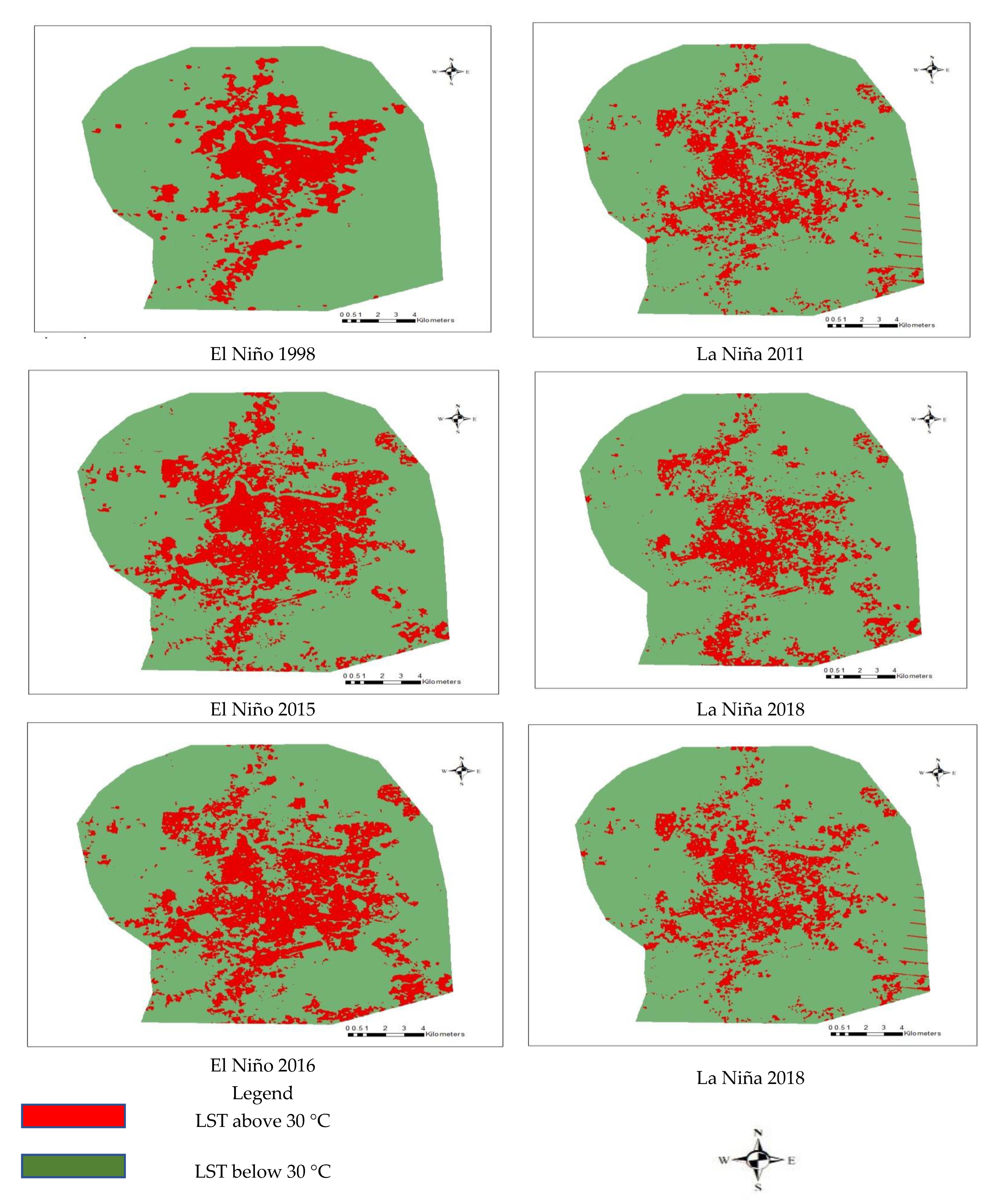
The distribution of surface temperatures exceeding 30 °C (heat concentration) during the La Niña and El Niño events is shown in Figure 9. Based on our observations, it is clear that the extent of concentrated hot areas during El Niño events is higher compared to that of La Niña events. Figure 9 provides a more detailed explanation of the differences in the extent of concentrated hot areas during the La Niña and El Niño events.

The left side of Figure 9 displays the temperature distribution during El Niño events, characterized by ONI values ranging from 2.2 to 2.6. On the right side of Figure 9, the temperature distribution during La Niña events is depicted, with negative ONI values ranging from −1.6 to −1.7. Based on the findings presented in Table 6, significant differences in the maximum, minimum, and average temperatures were observed between El Niño and La Niña events. During El Niño events, the average temperature showed a difference ranging from 3.51 to 4.71 °C, while the difference in the maximum temperature ranged from 2.06 to 4.6 °C, and the difference in the minimum temperature ranged from 5.36 to 6.65 °C. Table 6 also reveals that when the ONI values are between −1 and +1, indicating moderate strength, the maximum, minimum, and average temperatures are lower compared to the statistics derived from the MODIS satellite.

The extent of focal point areas of extreme heat during El Niño events is higher compared to that during La Niña events. During the El Niño events in 2015 and 2016, the areas of hotspots were 89.32 km² and 97.8 km², respectively, compared to the La Niña events in August 2018 and October 2018, which had clustered hotter areas of 61.23 km² and 59.73 km² (Figure 10). The pattern of the heat concentration area extent remains the same for the El Niño event in 1998, with a hot area of 89.32 km², compared to that of La Niña in 2011, which had an area of 55.82 km². This indicates the influence of ENSO on the change in the extent of the focal point areas of extreme heat. The increase in the nucleus heat area by 34 to 36 km² during El Niño events led to an increase in electricity usage by 20–30% from normal levels to balance the temperature in residential and office areas in Kuching City, Sarawak. These findings are supported by previous studies that state the increase in temperature during El Niño events is due to El Niño’s ability to raise global temperatures [1,5,32,33]. The indirect increase in global temperature can result in a local temperature increase, particularly in the study location. This is supported by Mou et al. [34], Maura et al. [14], and Song et al. [35], who state that the influence of local climate cannot affect the warming effect of El Niño when it is dominant, particularly at a mature stage. This explains why the statistical values of the maximum, minimum, and average temperatures, as well as the extent of hotter areas, are higher around Kuching City during El Niño compared to those during La Niña.

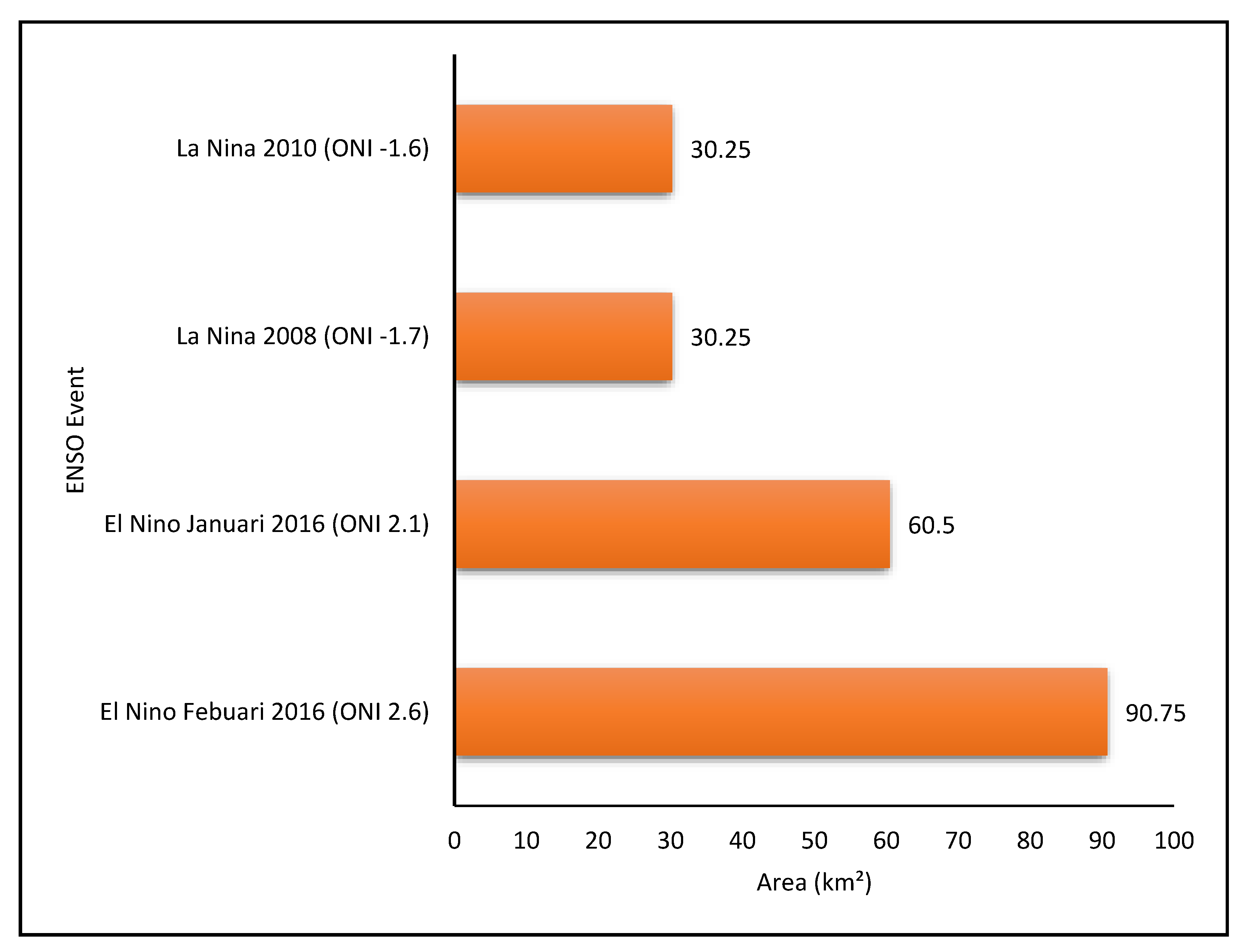
The extent of concentrated hot areas during El Niño events is higher compared to that during La Niña events (Figure 11). During the El Niño event in February 2016 with an ONI of 2.6 and in January 2016 with an ONI of 2.1, the respective cluster hotter areas were 90.75 km² and 60.5 km², compared to 30.25 km² during the La Niña events in 2008 and 2010. The extent of hotter areas during El Niño and La Niña events is consistent with the findings using the Landsat satellite, in which the extent of the focal point areas of extreme heat during El Niño is higher than that during La Niña events (Figure 11). The increase in hotspot areas during El Niño events will lead to an increased demand for electricity to compensate for the higher temperatures in residential and office areas in Kuching City, Sarawak.

The left side of Figure 9 displays the temperature distribution during El Niño events, characterized by ONI values ranging from 2.2 to 2.6. On the right side of Figure 9, the temperature distribution during La Niña events is depicted, with negative ONI values ranging from −1.6 to −1.7. Based on the findings presented in Table 7, significant differences in the maximum, minimum, and average temperatures were observed between El Niño and La Niña events. During El Niño events, the average temperature showed a difference ranging from 3.51 to 4.71 °C, while the difference in maximum temperature ranged from 2.06 to 4.6 °C, and the difference in minimum temperature ranged from 5.36 to 6.65 °C. Table 6 also reveals that when the ONI values are between −1 and 1, indicating moderate strength, the maximum, minimum, and average temperatures are lower compared to the statistics derived from the MODIS satellite.

Based on Table 6, the average temperatures during the El Niño events in 1997 and 1998 were 27.8 °C and 26.9 °C, respectively, while the average temperature during the La Niña events in November 2011 and September 2010 was 24 °C. This indicates a temperature difference of 2 to 3 °C between the ONI events. Kemarau and Eboy [36] state that rainfall decreases during El Niño events, which can lead to an increase in temperature, while high rainfall during La Niña events causes a decrease in temperature in Kuching City. Kemarau and Eboy [5,36] report that the effect of El Niño can cause a temperature increase ranging from 0.5 °C to 1.5 °C, while La Niña can cause a temperature decrease ranging from 0 °C to 1.2 °C. This explains why the extent of hotter areas during El Niño events is higher compared to that during La Niña events.

The findings of this study differ from the findings of Moura et al. [14], who studied the Amazon and reported a temperature difference of 7.5−8 °C between El Niño and La Niña events using MODIS data. The variation in the impact of ENSO events on the temperature in the study by Moura et al. [14] depends on factors such as topography, with higher temperatures observed in lowland areas compared to areas near the Andes Mountains. Kogan and Guo [15] also used MODIS data to study the effect of El Niño on global temperature and vegetation systems and found that El Niño resulted in temperature increases ranging from 0.5 to 2.50 °C depending on the location. The findings of Kogan and Guo [15] are similar to the findings of this study. The differences in temperature changes are due to factors such as topography and the location of the place studied, as stated by Kemarau and Eboy [5,36]. This demonstrates that remote sensing techniques can identify the effects of El Niño and La Niña events on the temperature distribution at the study location, namely Kuching City, Sarawak. Through remote sensing techniques, it was found that urban and industrial areas are concentrated hot areas. Concentrated hot areas refer to areas with surface temperatures exceeding 30 °C, which can cause discomfort to humans [31].

The use of Landsat satellite to study the effects of ENSO on the urban climate for selected data with strong ENSO magnitude values of −1 (La Niña) and 1 (El Niño) revealed a temperature increase of 2.10−2.80 °C. This explains the urban heat island effect in the temperature increase during El Niño events, which is 1.30−1.50 °C after subtracting the overall temperature increase pattern for Malaysia without considering the influence of the urban heat island effect on the temperature increase due to ENSO, as found in the study by Mou et al. [34]. The findings of this study are consistent with the findings of Tawang and Tengku [37], who reported temperature increases of 0.1−1.9 °C in Kedah and 0.1−2.4 °C in Perlis during the El Niño event of 1997, based on meteorological data.

On the other hand, areas near bodies of water and areas covered with vegetation are concentrated cool areas. Industrial areas are one of the concentrated hot areas and record the highest temperatures compared to those of the surrounding urban environment, as expected due to high heat emissions [38,39].

The industrial areas in the white-shaded areas in Figure 7 include zones H, I, J, and K. Additionally, urban areas become concentrated hot areas due to the presence of buildings and human-made structures, resulting in surface temperature increases [40]. Anthropogenic heating significantly contributes to the urban heat island effect, especially due to the use of air conditioning in buildings [41] in urban central areas. Urban areas represented by the black-shaded areas consist of zones B, C, D, E, F, and G [39]. Furthermore, Kemarau and Eboy [20] state that the emission of carbon dioxide (CO₂) and carbon monoxide (CO) in industrial areas contributes to temperature increases in the surrounding areas.

This study found that bodies of water and vegetated areas are concentrated cool areas, characterized by relatively lower temperatures. Previous studies such as those by Berger et al. [40], Coutts et al. [41], and Feyisa et al. [42] have also found that vegetation and bodies of water can reduce surface temperatures in urban areas. This explains why concentrated cool areas consist of bodies of water and vegetation. Examples of concentrated cool areas include water bodies such as the Sarawak River, as well as vegetation areas like wetland areas, botanical gardens, and Kuching Cultural City Forest.

Furthermore, the effect of bodies of water in mitigating temperature due to the urban heat island effect has been considered by a small number of researchers. The Normalized Difference Water Index (NDWI) has been studied by Kemarau and Eboy [38,39] using the Land Water Surface Index (LWSI) to investigate the relationship between bodies of water and the surface temperature in urban areas. Previous studies have found that the selected water indices have a positive relationship with the temperature, meaning that temperatures decrease as the index value increases. Additionally, the distance between bodies of water or coastlines and green areas affects the surface temperature, as proximity to water sources or green vegetation leads to lower surface temperatures [38,39,41,42].

4.2. Validation of LST MODIS and Landsat with MMD

Figure 4 displays the difference in correlation coefficients between meteorological temperature data and surface temperature obtained from the MODIS and Landsat satellites. The graph indicates a higher correlation value for the Landsat satellite (0.97) compared to that of the MODIS satellite (0.90). This difference can be attributed to the higher resolution of the Landsat (30 m) satellite compared to that of the MODIS (5600 m) satellite. These findings suggest that the data of both the Landsat and MODIS satellites accurately represent the surface temperature for studying the effects of ENSO on the temperature in Kuching City using remote sensing techniques. The accuracy of RS data and techniques in assessing the impact of ENSO events on temperature is 97% for Landsat and 90% for MODIS.

Referring to Figure 3 there are differences in daily temperatures between the MMD data and the daily temperatures derived from the Landsat satellite. This study found the largest difference in December 1995, with a negative (−) 1.7 °C difference. The second-largest difference occurred in August 2004, with a negative (−) 1.4 °C difference, followed by negative (−) 1.3 °C in February 2011 as well as negative (−) 1.2 °C in September 2005 and October 2005. These differences arise because RS sensors, such as Landsat and MODIS, measure surface temperature, while meteorological stations measure air temperature [43].

Overall, the Landsat RS data shows differences of lower than positive (+) 0.5 °C or negative (−) 0.5 °C. This indicates that 97% of the data have small differences below 0.5 °C. There is a positive relationship with a correlation coefficient of 0.97 between the Landsat RS data and temperature data from the MMD. This indicates that the majority of daily data from the MMD and the Landsat satellite have differences below positive (+) 0.5 °C or negative (−) 0.5 °C.

Regarding the differences between the monthly average temperatures from the MMD and the monthly average temperatures from MODIS (shown in Figure 12), the largest difference between the two datasets is observed in April 2008, with a positive (+) 1.2 °C difference. This is followed by a negative (−) 0.9 °C difference in January 2003, a positive (+) 0.9 °C difference in May 2006, and the third-largest difference of negative (−) 0.7 °C in July 2000. These differences arise because satellite RS, such as that by Landsat and MODIS, measures the surface temperature, whereas meteorological stations measure the air temperature [44]. This study found that nearly all of the 216 data points have differences below positive (+) 0.5 °C and negative (−) 0.5 °C. This means that 91% of MODIS data have differences of less than 0.5 °C compared to the MMD temperature data. This explains the positive correlation between the monthly temperatures from the MODIS satellite and the MMD, with a correlation coefficient (R) of 0.90.

The findings of this study are consistent with the study conducted by Hereher [44], which examined the effect of global warming on global temperature patterns using 273 MODIS images and meteorological data. Hereher [44] reported that global warming leads to an increase in global temperatures. In order to evaluate the accuracy and validity of the data, Hereher [44] compared MODIS data with meteorological data and found an 84% accuracy rate for MODIS data in measuring the temperature, with a correlation coefficient of 0.84 (R²) between the MODIS satellite surface temperature data and the temperature data from the meteorological department. This result is similar to the 90% correlation reported by Zhou et al. [6] and the 85% correlation reported by Varentsov et al. [45], both of whom also used MODIS or Landsat data. This explains why the correlation coefficient between the surface temperature from the MODIS or Landsat satellites and the temperature data from the MMD exceeds 0.80.

The correlation relationship between meteorological data (temperature) and the ONI (Oceanic Niño Index) as an indicator for assessing the effectiveness of RS (remote sensing) techniques and data in studying the impact of ENSO events on the temperature in Kuching, Sarawak is shown in Figure 13. We found a direct and positive correlation pattern between the surface temperature from the MODIS and Landsat satellites and the ONI. The correlation coefficients were 0.71 for the Landsat satellite and 0.73 for the MODIS satellite (Figure 4).

The findings of this study align with the research conducted by Nour Eldeen et al. [46], who also utilized MODIS data to measure temperatures in Africa and assessed their effectiveness in desert areas. Nour Eldeen et al. [46] reported a 90% accuracy rate for MODIS data in measuring temperatures in Africa, based on a correlation analysis with meteorological data. The correlation coefficient between the MODIS RS data and the temperature data from the MMD was 0.90, which is consistent with the findings of this study. This confirms that MODIS data are suitable for measuring surface temperature in desert and tropical regions. Both the Landsat and MODIS RS datasets have high correlation coefficients of 0.97 and 0.90, respectively, indicating their potential for studying land surface temperature characteristics in specific locations [13,14,15,46,47]. The quality of MODIS data undergoes rigorous processing and validation by experts, ensuring an accuracy rate of nearly 90% compared to that of the MMD’s temperature data. RS technology bridges data gaps in areas without weather stations, especially remote and inaccessible regions, allowing us to access weather and climate information related to global climate change. The findings of Garfinkel et al. [48] also support the conclusions of Nour Eldeen et al. [46], as they conducted a global-scale study with similar results.

The direct correlation between the ONI and air temperature over three months is shown in Figure 13, based on the ONI formula. The analysis includes 385 monthly average temperature data points from the MMD and ONI values from 1988 to 2019, organized in the format of three-month averages. The results reveal a strong positive correlation (R² = 0.75) between the ONI and temperature from the MMD, indicating the impact of ENSO events on air temperature. El Niño events, associated with increased temperatures, lead to drought and aridity, resulting in higher temperatures in Kuching, Sarawak. On the other hand, La Niña events, characterized by increased rainfall, lead to a decrease in temperature. Table 5 demonstrates a positive correlation between the ONI and the temperature from MODIS and Landsat satellites, although with slightly lower correlation coefficients (0.68 for MODIS and 0.71 for Landsat) compared to that of the MMD (0.75). Nonetheless, RS data remains effective in studying the relationship between the ONI and temperature, with correlation coefficients exceeding 50% (68% for MODIS and 71% for Landsat).

Changes in the ONI (Oceanic Niño Index) values are reflected in the temperature changes observed by the MODIS and Landsat satellites. When the ONI exceeds 0.5, indicating El Niño events, it corresponds to increased temperatures. On the other hand, La Niña events lead to decreased temperatures due to increased rainfall. These findings align with previous studies, such as those by Drosdowsky [49] and Kemarau and Eboy [4,5], which reported similar effects of rainfall on temperature. El Niño events cause drought and below-average rainfall, resulting in temperature increases. Conversely, the increased rainfall during La Niña events contributes to a temperature reduction. El Niño conditions also shorten the monsoon season, leading to lower rainfall. Furthermore, Freychet et al. [50] found that the highest meteorological temperatures occurred during the peak of the 2015 El Niño, which can be attributed to the heat absorption and release properties of building materials.

The average monthly temperature during normal or neutral conditions is 26 °C when the ONI is between −0.5 and 0.5. Based on Figure 14, it can be observed that monthly temperature changes depend on the type of ENSO event. For example, during the El Niño events of 1997–1998 and 2015/2016, temperature increases were observed. The El Niño event of 1997–1998 caused a temperature change of 1.8 °C, while the El Niño event of 2015/2016 saw an increase of 2.5 °C. Overall, this study found that El Niño events caused temperature increases ranging from 0.5 °C to 1.5 °C based on RS data and data provided by the Kuching Meteorological Station. On the other hand, temperature decreases ranged from 0 °C to 1.2 °C during La Niña events. Thus, it was found that El Niño events caused temperature increases, while La Niña events caused temperature decreases in Kuching, Sarawak [4,5].

In the context of meteorological data, it was found that Malaysia as a whole experienced a general increase in temperature of 0.38 to 0.5 °C [51]. Previous studies reported an average temperature increase of 0.09 to 0.34 °C per decade from 1971 to 2001 [52]. Similarly, Tangang et al. [52] found a similar increase of 0.27 to 0.40 °C per decade between 1961 and 2002 in Peninsular Malaysia and Northern Borneo. Comparing the findings of these studies, it was found that the urban heat island effect contributed to a 2 °C increase.

On a global scale, Lin et al. [3] confirmed that El Niño has caused temperature increases in Indochina ranging from 0.53 °C to 0.60 °C during peak El Niño periods. The study by Lin et al. (2018) also found that El Niño events weakened the northeast Monsoon season. This statement was also supported by Luo and Lau [53], who found that El Niño events caused a general temperature increase of 0.50 to 0.65 °C. Lin et al. [1] also stated that El Niño events led to heatwaves in Indochina, resulting in higher surface temperatures than usual. This was due to reduced rainfall in Indochina during El Niño compared to La Niña. These findings align with previous studies, such as those of Lin et al. [1] and Lou and Lau [53]. Comparing the findings of these studies, it was found that the urban heat island effect contributed to a 2 °C increase.

This study’s findings are also similar to those of Kogan and Guo [15], who studied the effects of El Niño on global plant systems and climate and found that the 2015/2016 El Niño event caused temperature increases ranging from 0.5 to 2.50 °C depending on the location. The conclusion is that the effect of ENSO events on the temperature in Kuching City, Sarawak is that El Niño events lead to an increase in temperature, while La Niña events result in a decrease in temperature. For example, during the El Niño event in 2015/2016, there was an increase in temperature ranging from 0.5 to 1.5 °C. Additionally, in 2009 and 1997–1998, El Niño events also caused temperature increases of 0.5 to 1.5 °C. The temperature increase during El Niño is due to a decrease in rainfall in the study area, resulting in drought conditions. In 2009, the temperature increased due to a 25–30% decrease in rainfall in the Kuching City area [36].

5. Conclusions

This study aimed to investigate the impact of ENSO on temperature using remote sensing (RS) data. Our key findings revealed that ENSO events have a significant effect on the surface temperature, as observed through the Landsat and MODIS satellite data during El Niño and La Niña events. The surface temperature was found to be influenced by the Oceanic Niño Index (ONI), with El Niño events leading to a temperature rise of 0.5–2.5 °C when the ONI value exceeded +0.5. The study also analyzed the impact of ENSO on the spatial distribution of the surface temperature in Kuching City, Sarawak and found that ENSO events affect both the maximum and average temperatures in the city.

The effectiveness of RS data from the MODIS and Landsat satellites in studying the impact of ENSO events on the surface temperature in Kuching City was assessed, revealing a high effectiveness with correlation coefficients of 0.97 for the MODIS satellite data and 0.90 for the Landsat satellite data when compared to temperature data provided by the Kuching branch of the Malaysian Meteorological Department (MMD). These findings have important implications for stakeholders and the community in Kuching City, enhancing public awareness of the threats posed by temperature increases during ENSO events. This study also highlights temperature variations in different areas of the city, emphasizing the need for preparedness measures to mitigate the effects of urban heat islands and ENSO on the local environment. This knowledge is crucial for disaster management agencies, such as the Sarawak State Disaster Management Committee, natural disaster management agencies, and the National Security Council, enabling them to implement targeted steps and assistance in hotspot areas such as industrial zones and city centers to reduce the impact of ENSO on the community.

However, this study had limitations primarily due to its reliance on MODIS and Landsat satellite data, which require cloud-free study locations. Cloud cover poses a persistent challenge in Malaysia’s equatorial climate, obstructing thermal wave measurements and leading to data loss. Therefore, collecting RS data comprehensively and accurately remains difficult. For future research, it is recommended to utilize high-resolution data, such as drones/UAVs with a resolution of 1 m or less, which can provide more detailed information, particularly for studying the effects of ENSO events on built-up areas. Additionally, researchers anticipate the availability of satellites with high-resolution thermal wave capabilities in the future, enabling more precise, detailed, and long-term investigations into the impact of ENSO on urban climates.

References

1. Lin, L.; Chen, C.; Luo, M. Impacts of El Niño–Southern Oscillation on heat waves in the Indochina peninsula. Atmos. Sci. Lett. 2018, 19, e856. [Google Scholar] [CrossRef] [Green Version]
2. Sum, L.P. El-Niño: A Review of Scientific Understanding and the Impact of 1997/98 Event in Malaysia; Sum, L.P., Tangang, F., Eds.; Academy of Sciences: Warsaw, Poland, 2018; Volume 20. [Google Scholar]
3. Thirumalai, K.; DiNezio, P.N.; Okumura, Y.; Deser, C. Extreme temperatures in Southeast Asia caused by El Niño and worsened by global warming. Nat. Commun. 2017, 8, 15531. [Google Scholar] [CrossRef] [PubMed] [Green Version]
4. Kemarau, R.A.; Eboy, O.V. The Impact of El Niño–Southern Oscillation (ENSO) on Temperature: A Case Study in Kuching, Sarawak. Malays. J. Soc. Sci. Humanit. 2021, 6, 289–297. [Google Scholar] [CrossRef]
5. Kemarau, A.R.; Eboy, O.V. The influence of El Niño Southern Oscillation on urban heat island formation at tropical city: Case of Kuching City, Sarawak. Malays. J. Soc. Space 2021, 17, 288–304. [Google Scholar]
6. Zhou, D.; Xiao, J.; Bonafoni, S.; Berger, C.; Deilami, K.; Zhou, Y.; Frolking, S.; Yao, R.; Qiao, Z.; Sobrino, J.A. Satellite Remote Sensing of Surface Urban Heat Islands: Progress, Challenges, and Perspectives. Remote Sens. 2018, 11, 48. [Google Scholar] [CrossRef] [Green Version]
7. Kovacs, P.; Kunreuther, H. Managing Catastrophic Risk: Lessons from Canada; Institute for Catastrophic Loss Reduction: Toronto, ON, Canada, 2001. [Google Scholar]
8. Sharma, J.; Ravindranath, N.H. Applying IPCC 2014 framework for hazard-specific vulnerability assessment under climate change. Environ. Res. Commun. 2019, 1, 051004. [Google Scholar] [CrossRef]
9. Clay, R.; Guan, H.; Wild, N.; Bennett, J.; Vinodkumar; Ewenz, C. Urban Heat Island traverses in the City of Adelaide, South Australia. Urban Clim. 2016, 17, 89–101. [Google Scholar] [CrossRef]
10. Mirzaei, P.A.; Haghighat, F. Approaches to studying urban heat island–abilities and limitations. Build. Environ. 2010, 45, 2192–2201. [Google Scholar] [CrossRef]
11. Smoliak, B.V.; Snyder, P.K.; Twine, T.E.; Mykleby, P.M.; Hertel, W.F. Dense Network Observations of the Twin Cities Canopy-Layer Urban Heat Island. J. Appl. Meteorol. Clim. 2015, 54, 1899–1917. [Google Scholar] [CrossRef]
12. Wang, S.; Ma, Q.; Ding, H.; Liang, H. Detection of urban expansion and land surface temperature change using multi-temporal landsat images. Resour. Conserv. Recycl. 2018, 128, 526–534. [Google Scholar] [CrossRef]
13. Eboy, O.V.; Kemarau, R.A. Study Variability of the Land Surface Temperature of Land Cover during El Niño Southern Oscillation (ENSO) in a Tropical City. Sustainability 2023, 15, 8886. [Google Scholar] [CrossRef]
14. Moura, M.M.; Dos Santos, A.R.; Pezzopane, J.E.M.; Alexandre, R.S.; da Silva, S.F.; Pimentel, S.M.; de Andrade, M.S.S.; Silva, F.G.R.; Branco, E.R.F.; Moreira, T.R.; et al. Relation of El Niño and La Niña phenomena to precipitation, evapotranspiration, and temperature in the Amazon basin. Sci. Total Environ. 2019, 651, 1639–1651. [Google Scholar] [CrossRef] [PubMed]
15. Kogan, F.; Guo, W. Strong 2015–2016 El Niño and implication to global ecosystems from space data. Int. J. Remote Sens. 2017, 38, 161–178. [Google Scholar] [CrossRef]
16. Kuok, K.K.; Chiu, P.C. Space-saving rainwater harvesting tanks for double-story houses in Kuching, Sarawak. Int. J. Eng. Technol. 2019, 8, 38–43. [Google Scholar]
17. Mahmud, M. Peristiwa El Niño dan pengaruh IOD terhadap hujan di Malaysia. e-BANGI 2018, 13, 166–177. [Google Scholar]
18. Available online: https://earthexplorer.usgs.gov/ (accessed on 23 September 2019).
19. Available online: https://ladsweb.modaps.eosdis.nasa.gov/search/ (accessed on 18 September 2019).
20. Wan, Z.; Zhang, Y.; Wang, R.; Li, Z. Early Land-Surface Temperature Product Retrieved from MODIS Data. IGARSS 2001, 3, 1067–1069. Available online: https://bit.ly/2V3SllY (accessed on 26 December 2018).
21. Available online: https://origin.cpc.ncep.noaa.gov/products/analysis_monitoring/ensostuff/ONI_v5.php (accessed on 7 July 2023).
22. Kemarau, R.A.; Eboy, O.V. Urbanization And Its Impacts On Land Surface Temperature On Small Medium Size City For Years 1991, 2011 And 2018: Case Study Kota Kinabalu. J. Borneo Soc. Transform. Stud. 2020, 6, 957. [Google Scholar] [CrossRef]
23. Emmanuel, P.B.; Pateraki, M.N.; Zhang, L. Radiometric and geometric evaluation of Ikonos GEO images and their use for 3D building modeling. In Joint Workshop of ISPRS Working Groups I/2, I/5, and IV/7 High-Resolution Mapping from Space 2001; ETH Hönggerberg, Institute of Geodesy and Photogrammetry: Singapore, 2001. [Google Scholar]
24. Young, S.J.; Johnson, B.R.; Hackwell, J.A. An in-scene method for atmospheric compensation of thermal hyperspectral data. J. Geophys. Res. Atmos. 2002, 107, ACH-14. [Google Scholar] [CrossRef]
25. Gyanesh, C.; Markham, B.L.; Helder, D.L. Summary of current radiometric calibration coefficients for Landsat MSS, TM, ETM+, and EO-1 ALI sensors. Remote Sens. Environ. 2009, 113, 893–903. [Google Scholar]
26. Artis, D.A.; Carnahan, W.H. Survey of emissivity variability in thermography of urban areas. Remote Sens. Environ. 1982, 12, 313–329. [Google Scholar] [CrossRef]
27. He, J.; Zhao, W.; Li, A.; Wen, F.; Yu, D. The impact of the terrain effect on land surface temperature variation based on Landsat-8 observations in mountainous areas. Int. J. Remote Sens. 2019, 40, 1808–1827. [Google Scholar] [CrossRef]
28. Zhi-Hao, Q.; Zhang, M.-H.; Karnieli, A.; Berliner, P. Mono-window algorithm for retrieving land surface temperature from Landsat TM6 data. Acta Geogr. Sin. 2001, 56, 456–466. [Google Scholar]
29. Carlson, T.N.; Ripley, D.A. On the relation between NDVI, fractional vegetation cover, and leaf area index. Remote Sens. Environ. 1997, 62, 241–252. [Google Scholar] [CrossRef]
30. De Sá, J.P. Applied Statistics Using SPSS, Statistica, MatLab, and R; Springer Science & Business Media: Berlin/Heidelberg, Germany, 2007. [Google Scholar]
31. Baum, S.; Horton, S.; Low Choy, D.; Gleeson, B. Climate change, health impacts, and urban adaptability: A case study of Gold Coast City. Res. Monogr. 2009, 11, 68. [Google Scholar]
32. Min, S.K.; Cai, W.; Whetton, P. Influence of climate variability on seasonal extremes over Australia. J. Geophys. Res. Atmos. 2013, 118, 643–654. [Google Scholar] [CrossRef]
33. Chen, R.; Wen, Z.; Lu, R. Large-Scale Circulation Anomalies and Intraseasonal Oscillations Associated with Long-Lived Extreme Heat Events in South China. J. Clim. 2017, 31, 213–232. [Google Scholar] [CrossRef]
34. Tan, M.L.; Juneng, L.; Tangang, F.T.; Chung, J.X.; Firdaus, R.B.R. Changes in temperature extremes and their relationship with ENSO in Malaysia from 1985 to 2018. Int. J. Clim. 2020, 41, E2564–E2580. [Google Scholar] [CrossRef]
35. Yang, S.; Li, Z.; Yu, J.-Y.; Hu, X.; Dong, W.; He, S. El Niño–Southern Oscillation and its impact in the changing climate. Natl. Sci. Rev. 2018, 5, 840–857. [Google Scholar] [CrossRef] [Green Version]
36. Kemarau, R.A.; Eboy, O.V. Application Remote Sensing in Study Influence of El Niño Incident in 2015/2016 on the Amount of Rainfall in Sarawak. J. Techno-Soc. 2021, 13, 12–22. [Google Scholar]
37. Tawang, A.B.; Tengku Ahmad, T.A.B.; Abdullah, M. Stabilization of Upland Agriculture under El Nino-Induced Climatic Risk: Impact Assessment and Mitigation Measures in Malaysia, Working Paper No. 61; CGPRT Centre: Bogor, Indonesia, 2002. [Google Scholar]
38. Kemarau, R.A.; Eboy, O.V. Analyses Water Bodies Effect in Mitigation of Urban Heat Effect: Case Study Small Size Cities Kuching, Sarawak. In IOP Conference Series: Earth and Environmental Science; IOP Publishing: Bristol, UK, 2020; Volume 540, p. 012010. [Google Scholar]
39. Kemarau, R.A.; Eboy, O.V. Spatial-Temporal of Urban Green Space in Tropical City Of Kuching, Sarawak, Malaysia. J. Appl. Sci. Process Eng. 2021, 8, 660–670. [Google Scholar] [CrossRef]
40. Berger, C.; Rosentreter, J.; Voltersen, M.; Baumgart, C.; Schmullius, C.; Hese, S. Spatio-temporal analysis of the relationship between 2D/3D urban site characteristics and land surface temperature. Remote Sens. Environ. 2017, 193, 225–243. [Google Scholar] [CrossRef]
41. Coutts, A.M.; Harris, R.J.; Phan, T.; Livesley, S.J.; Williams, N.S.G.; Tapper, N.J. Thermal infrared remote sensing of urban heat: Hotspots, vegetation, and an assessment of techniques for use in urban planning. Remote Sens. Environ. 2016, 186, 637–651. [Google Scholar] [CrossRef]
42. Feyisa, G.L.; Dons, K.; Meilby, H. Efficiency of parks in mitigating urban heat island effect: An example from Addis Ababa. Landsc. Urban Plan. 2014, 123, 87–95. [Google Scholar] [CrossRef]
43. United States Of America (USA) Environmental Protection Agency. 2020. Available online: https://www.epa.gov/sites/production/files/2014-06/documents/basicscompendium.pdf (accessed on 1 September 2019).
44. Hereher, M.E. Effect of land use/cover change on land surface temperatures—The Nile Delta, Egypt. J. Afr. Earth Sci. 2017, 126, 75–83. [Google Scholar] [CrossRef]
45. Varentsov, M.I.; Grishchenko, M.Y.; Wouters, H. Simultaneous assessment of the summer urban heat island in Moscow megacity based on in situ observations, thermal satellite images and mesoscale modeling. Geogr. Environ. Sustain. 2019, 12, 74–95. [Google Scholar] [CrossRef] [Green Version]
46. NourEldeen, N.; Mao, K.; Yuan, Z.; Shen, X.; Xu, T.; Qin, Z. Analysis of the Spatiotemporal Change in Land Surface Temperature for a Long-Term Sequence in Africa (2003–2017). Remote Sens. 2020, 12, 488. [Google Scholar] [CrossRef] [Green Version]
47. Naeem, S.; Cao, C.; Qazi, W.A.; Zamani, M.; Wei, C.; Acharya, B.K.; Rehman, A.U. Studying the Association between Green Space Characteristics and Land Surface Temperature for Sustainable Urban Environments: An Analysis of Beijing and Islamabad. ISPRS Int. J. Geo-Inf. 2018, 7, 38. [Google Scholar] [CrossRef] [Green Version]
48. Garfinkel, C.I.; Butler, A.H. Reviews of Geophysics the Teleconnection of el Niño Southern Oscillation to the Stratosphere. Rev. Geophys. 2018, 57, 547. [Google Scholar]
49. Drosdowsky, W.; Wheeler, M.C. Predicting the Onset of the North Australian Wet Season with the POAMA Dynamical Prediction System. Weather. Forecast. 2014, 29, 150–161. [Google Scholar] [CrossRef]
50. Freychet, N.; Sparrow, S.; Tett, S.F.B.; Mineter, M.J.; Hegerl, G.C.; Wallom, D.C.H. Impacts of Anthropogenic Forcings and El Niño on Chinese Extreme Temperatures. Adv. Atmos. Sci. 2018, 35, 994–1002. [Google Scholar] [CrossRef] [Green Version]
51. Tangang, F.T.; Juneng, L.; Ahmad, S. Trend and interannual variability of temperature in Malaysia: 1961–2002. Theor. Appl. Clim. 2006, 89, 127–141. [Google Scholar] [CrossRef]
52. Wai, N.M.; Camerlengo, A.; Wahab, A.K. A study of global warming in Malaysia. J. Teknol. 2005, 42, 1. [Google Scholar]
53. Luo, M.; Lau, N.-C. Amplifying effect of ENSO on heat waves in China. Clim. Dyn. 2019, 52, 3277–3289. [Google Scholar] [CrossRef]
Figure 1. Location of study (Google Earth).
Applsci 13 08861 g001
Figure 2. Flowchart steps to achieve the objectives of the study.
Applsci 13 08861 g002
Figure 3. Difference in daily temperature values with LST (land surface temperature) from the Landsat satellite.
Applsci 13 08861 g003
Figure 4. The correlation between land surface temperature (LST) derived from Landsat, LST from MODIS, and the Oceanic Niño Index (ONI).
Applsci 13 08861 g004
Figure 5. ONI time series and air temperature during 1988−2019.
Applsci 13 08861 g005
Figure 6. Correlation analysis between ONI and air temperature.
Applsci 13 08861 g006
Figure 7. LST distribution during El Niño and La Niña from Landsat.
Applsci 13 08861 g007aApplsci 13 08861 g007b
Figure 8. LST distribution during El Niño and La Niña from MODIS.
Applsci 13 08861 g008
Figure 9. The areas with surface temperatures exceeding 30 °C during La Niña and El Niño events in Kuching City can be observed from Landsat satellite data.
Applsci 13 08861 g009
Figure 10. Areas of land surface temperature Landsat above 30 °C.
Applsci 13 08861 g010
Figure 11. The area of hotter areas during El Niño events is higher compared to that during La Niña events based on MODIS data.
Applsci 13 08861 g011
Figure 12. Temperature differences between LST (land surface temperature) MODIS satellite data and MMD (Malaysian Meteorological Department) data.
Applsci 13 08861 g012
Figure 13. Direct correlation between ONI (Oceanic Niño Index) and air temperature from MMD over three months based on the ONI formula.
Applsci 13 08861 g013
Figure 14. The monthly mean temperature pattern changes from MMD from 1988 to 2019 in the city of Kuching.
Applsci 13 08861 g014