Abstract
To address the complexity of siting and sizing for the renewable energy and energy storage (ES) of offshore oil–gas platforms, as well as to enhance the utilization of renewable energy and to ensure the power-flow stability of offshore oil–gas platforms, this paper proposes a hierarchical clustering-and-planning method for wind turbine (WT)/photovoltaic (PV) ES. The proposed strategy consists of three stages. First, the WT/PV power generation is forecast by a LightGBM model. The WT/PV siting and sizing at each node of the distribution network is optimized with a particle swarm optimization (PSO) algorithm, with the objectives of economy and stability. In the second stage, the distribution network is partitioned into sub-clusters, based on a voltage and loss-sensitivity index. Finally, the ES siting and sizing is optimized with PSO to minimize the line loss and the voltage fluctuation for each sub-cluster. The relationship between the economic and stability indicators is conducted quantitatively in the joint-planning approach. Considering the 10 kV distribution network of an oil–gas platform in the Bohai Sea of China as an example, our experiments demonstrated that by adjusting the WT/PV ES capacity for different gas-turbine power outputs, line losses can be reduced by 55–66% and voltage fluctuations can be reduced by 30.4–47.5%.
1. Introduction
In recent years, offshore oil–gas platforms have tended to reduce carbon emissions. Currently, the joint power-supply technology of renewable energy and traditional energy is being explored. As an abundant but unstable renewable-energy source, offshore wind power has the advantages of high average wind speed, high utilization hours, and easy large-scale development. Since offshore solar energy complements wind energy [1,2], offshore wind turbine (WT) and photovoltaic (PV) units have become global hotspots at the frontier of renewable energy development [3,4,5]. As the number of WT/PV units increases, energy storage (ES) systems with a two-way energy-flow capacity must be properly introduced to reduce the impact of the instability of WT/PV output on a power system [6]. Therefore, to achieve the low-carbon-emission goal for offshore oil–gas platforms, it is necessary to introduce WT/PV ES into the existing offshore oil field power grid to form a power-supply mode of new-energy access, multi-energy complementation, and low-carbon operation, which is necessary for the future construction of “carbon-neutral” oil fields.
Recently, many scholars studied the method of WT/PV ES for distribution networks and proposed a variety of distributed generation (DG) and ES optimization methods. In [7], the siting and sizing of DG were divided into two levels. The first level considered line losses and voltage fluctuations and the second level considered the income of operators. In [8], an PV ES-capacity-optimization model was established with the goal of optimizing the loss-of-load probability and the energy-overflow ratio, but the influence of line loss was not considered in the capacity planning. In [9], a distribution network with numerous nodes was divided into clusters. That study proposed an initial planning of the capacity of each cluster, with the cluster as the unit and a reduction in the comprehensive cost as the goal, followed by the planning of the capacity of each node, with the node as the unit and reducing line loss as the goal. In [10], a heuristic strategy based on voltage sensitivity was proposed to realize the optimal planning of ES to solve the voltage-limit violation of a distribution network upon the connecting of DG to the distribution network. A particle swarm optimization (PSO) algorithm was employed in [11,12,13,14] to determine the location and capacity of a single DG unit or multiple DG units, focusing on optimizing voltage fluctuation and line losses. However, ES was not considered. A model was developed in [15] to optimize ES capacity planning by considering investment costs and battery lifespan to achieve overall economic efficiency. An improved particle swarm optimization (IPSO) algorithm was used in [16] to optimize energy storage capacity, with the objectives of minimizing voltage fluctuations and enhancing economic factors. However, the siting of ES was not considered. A model based on multiple scenarios for siting and sizing for PV and ES planning was established in [17], and the planning problem was solved by a centroid opposition-based learning-particle swarm optimization (COBL-PSO) algorithm; however, that study did not consider multiple forms of DGs.
These studies established reasonable planning methods for the connection of DG to a distribution network and effectively improved the penetration rate of new energy in a distribution network, but they did not consider the offshore situation. The marine environment is very harsh, with a high salt–fog concentration, high humidity, and the possibilities of extreme cold, high heat, typhoons, tsunamis, and other disastrous events [18]. When WT, PV, and other power-generation equipment are located offshore in a marine environment, corrosion and aging are significantly accelerated by the harsh conditions. Compared with land equipment, offshore equipment is more likely to fail, leading to equipment downtime. From the perspective of power flow, it is likely that the failure of a power-generation unit in the power grid will lead to a voltage-limit violation of the distribution network, an active-power-limit violation of the line, and load loss [19], which will have a huge impact on the stable operation of offshore oil–gas platform clusters. Hence, there must be stricter requirements for determining the siting and sizing of offshore renewable energy.
In view of the shortcomings of the existing research, this study describes a method to improve voltage stability and reduce line losses by siting and sizing WT/PV ES to increase the renewable-energy penetration of offshore oil and gas platforms. The optimization strategy comprehensively considers the static power-flow voltage stability, the principle of cluster partition, the initial investment budget, and other indicators. The strategy can be briefly summarized as follows:
- The first stage is capacity optimization for WT and PV. After obtaining the forecasting of wind and solar resources based on the prediction model of the LightGBM network, the WT/PV-connected capacity at each node of the distribution network is optimized, with the goals of power-flow stability and economy.
- The second stage is cluster partition. Sensitivity analysis is carried out on the distribution network after WT/PV planning. The voltage and line-loss sensitivity of each node is calculated and nodes with similar impacts are grouped into sub-clusters.
- The third stage is the optimization of ES planning. Taking each sub-cluster as a unit, the optimal location of ES is determined according to the sensitivity-analysis method and, then, the optimal capacity planning of ES is carried out with the goals of minimizing voltage fluctuation, reducing active power loss, and achieving optimal capacity.
- An algorithm based on a PSO algorithm and a power-flow calculation are used to solve the optimal planning of WT/PV ES following the methods of gas-turbine power constraints and economical constraints for an existing offshore oil-gas platform distribution network. The feasibility of offshore WT/PV ES for an offshore oil-gas platform is assessed.
Here, we considered the example of an oil-gas platform in the Bohai Sea of China. With proper manipulation of the WT/PV ES capacity, based on various gas-turbine power outputs, we achieved a 55–66% reduction in line losses and a 30.4–47.5% decrease in voltage fluctuations.
2. Modeling of Offshore Oil and Gas Platform Cluster System
The offshore oil–gas platform cluster mentioned in this paper refers to the electrification- and information-based power-supply system composed of offshore wind power, PV power, gas, load, and ES. Based on the original gas-turbine and conventional-power distribution network, the system incorporates distributed energy such as WT, PV, and ES, forming a unique electrification cluster power-supply mode for offshore oil–gas platforms that integrates renewable energy and traditional energy. To explore the outputs of different power sources, the DG model is analyzed as follows:
2.1. Wind-Turbine Model
The output power of a WT is affected by wind speed and the maximum power of WT, which can be described by a linear approximation equation [20]:
where Pw is the output power of the wind turbine, x is the actual wind speed, M is the maximum power of the WT, α and β are linear parameters, and vci, vco, and vr denote the cut-in wind speed, cut-out wind speed, and rated wind speed, respectively.
2.2. Photovoltaic Model
PV power generation is mainly affected by temperature and solar intensity. The PV-output power model can be established as follows [21]:
where Ps and Ppv are the PV-output power and the actual PV-output power under standard conditions (illumination intensity of 1000 W/m2, temperature of 25 °C), respectively; Gs and Ga are the illumination intensity and the actual illumination intensity under standard conditions, respectively; Tr and Ta are the nominal temperature (25 °C) and the actual temperature of PV, respectively; and k is the power–temperature coefficient.
2.3. Energy Storage Model
ES can enable the voltage of distribution network nodes to be adjusted, reduce losses, and improve the stability of the power grid. The charge/discharge state of charge (SOC) model of ES is as follows [21]:
where σ is the self-discharge rate of ES; ηc and ηd are the charging and discharging efficiencies of ES, respectively; Eess is the ES capacity; t is the time; Δt is a scheduling cycle; and Pch and Pdis are the charging and discharging powers of ES, respectively.
2.4. Topology Model
The cluster distribution network of offshore oil–gas platforms with n nodes is shown in Figure 1.
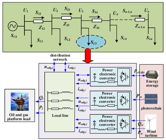
Figure 1.
A cluster-distribution network with n nodes for offshore oil–gas platforms.
In Figure 1, SG1 is the apparent power of the upper distribution network, Zi−1,i denotes the line impedance from node i − 1 to node i, Ui is the voltage of node i, Si−1,i is the line-flow power from node i − 1 to node i, Si is the apparent injection power of node i, and SLi is the sum of the load power Pl/Ql of node i and the connected power of the distributed generation units. WT/PV ES and other distributed generation units are connected to the local line through the power electronic converter and supply power to the load of the offshore oil–gas platform, together with the distribution network. The excess renewable energy can also be transmitted through the distribution network to supply power for other loads.
The injection power of any node m and the flow power between nodes can be derived from Figure 1:
where ΔSi is the power loss of the line, which can be expressed as follows:
where Ui is the voltage amplitude of node i; Pi and Qi are the injected active and reactive powers, respectively, of node i; and Ri−1,i and Xi−1,i are the resistance and reactance, respectively, between nodes i − 1 and i.
Node 1 is a slack bus, and the voltage of node m can be expressed as follows:
2.5. Prediction of Typical Output of Wind/Sunlight
LightGBM was first proposed in 2017. It inherits the practice of the XGBoost integration model and continuously performs residual fitting on multiple regression trees to integrate strong regression trees. Because of its fast running speed and high accuracy, it is becoming widely used.
To predict the typical daily output power of an offshore WT/PV system, based on the local wind meteorologically typical day, the PV meteorologically typical day, the historical meteorological data of the existing wind-farm solar field, and the corresponding power generation data, this study trained the WT and PV meteorologically typical daily-output power-prediction model based on the LightGBM network and, then, used the trained prediction model to predict the typical daily power generation according to the meteorologically typical days. The meteorological data of wind-power generation prediction included wind speed at different heights and wind direction corresponding to each wind speed, temperature, and humidity. Meteorological data for PV power generation prediction included short-wave radiation intensity, long-wave radiation intensity, cloud cover, temperature, and humidity.
The LightGBM prediction model can be expressed as follows:
where fw/pv refers to the prediction model of wind-power or PV-power generation based on LightGBM, and Xi is the i-th meteorological sample point for wind-power or PV-power generation. is the predicted generation power corresponding to the i-th sample point.
The objective function of the training was to minimize the mean square value (MSE) of prediction, as follows:
where Pi is the real power generation corresponding to sample i and N is the number of samples.
Finally, the trained wind-power-generation prediction model fw and the PV-power-generation prediction model fpv were used, respectively, to predict the wind-power generation and the PV-power generation on a typical day.
Xwind and Xpv denote the meteorological weather forecasting data used to predict the wind- and solar-power generation of a typical day, respectively, and their corresponding power predictions are determined by the following equations:
where Xw,i and Xpv,i are the i-th sample points of meteorological wind power and meteorological solar power of a typical day, respectively.
The reasonable prediction of local wind/solar sequential-power generation can provide a reasonable basis for the connected capacity of WT and PV cells. It can also guide the siting and sizing of ES to effectively reduce the system’s power fluctuation and line loss, stabilize the voltage, achieve the dispatching balance relationship (as shown in Equation (11)), improve the timing matching of each power supply in the system, and reduce the impact of the randomness of wind and solar energy, while improving the penetration of new energy:
where PG and PP are the dispatching output power of the gas-turbine and power grids, respectively, Pe,i is the ES dispatching output power, PL is the load-power forecasting, and npv/nw/ne are the total numbers of PV/WT ES, respectively. The ideal planning operation results are shown in Figure 2.
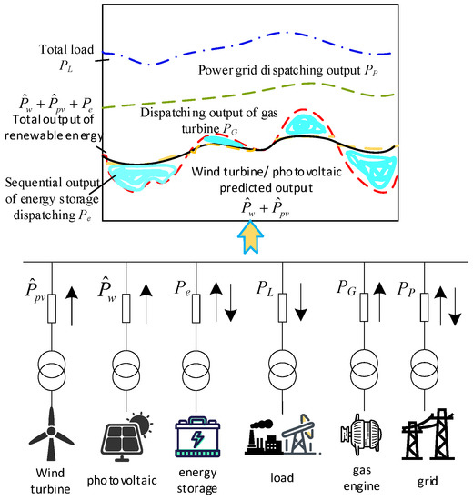
Figure 2.
Combined power supply structure of renewable and traditional power sources.
3. Stability Analysis and Cluster-Partition Principles of Offshore Oil–Gas Platform Cluster System
3.1. Stability Analysis
In [22], Jasmon proposed a method to judge the stability of power flow, mainly by studying the power and the line-impedance between the nodes of the distribution-network branch to judge whether the power flow had a solution. However, in the derivation process, the simple equivalent of the complex distribution network, from the perspective of loss, led to large errors and the influence of voltage fluctuation was not considered. Therefore, some scholars proposed an improved derivation of power-flow stability [23], which can more comprehensively reflect the power-flow relationship between nodes and more accurately judge the existence of power-flow solutions. The expression of static voltage-stability indicator Lij of the branches between nodes i and j is as follows:
where Ui is the voltage amplitude of node i; Pj and Qj are the injected active power and reactive power, respectively, of node j; and Rij and Xij are the resistance and reactance, respectively, between nodes i and j. When Lij < 1, the branch power flow is solvable and stable. The smaller the value of Lij, the greater the stability margin of the branch. When Lij > 1, the branch power flow has no solution and the power flow is unstable.
For a distribution network with n nodes, the static voltage-stability indicator of the whole distribution network should be the maximum value of the stability indicator Lij of all branches:
L denotes the weakest branch of the whole distribution network, which can reflect the stability of the whole distribution network, since voltage collapse in the system must start from the weakest branch.
3.2. Sensitivity Analysis
3.2.1. Voltage Sensitivity
If the line loss is ignored, the injected active power and reactive power of any node can be obtained:
Combining Equations (6) and (7) to simplify the expression, let
Then, the relationship between node-voltage change and power change can be obtained:
In Equation (16), the partial derivative of the voltage of any node m to the power of any node k can be expressed as follows:
The two Jacobian matrices in Equation (16) are called voltage-sensitivity matrices, and the sum of the absolute values of their row vectors represents the influence of the power changes of different nodes on the voltage of the same node. The larger the result, the more vulnerable the node voltage is to the power changes. The sum of the column vectors represents the influence of the power change of the same node on the voltage of other nodes. The larger the result, the greater the influence of the power of this point on the voltage of the whole system node.
3.2.2. Loss Sensitivity
According to Equation (6), the distribution network loss with n nodes can be expressed as follows:
To simplify the expression, let
Then, the relationship between the change-of-system loss and the change of power can be obtained as follows:
where
From Equations (19) and (20), it can be determined that in a distributing network with radial topology, the loss sensitivity is strongly related to the node injection power. The greater the absolute value of the node injection power, the greater the sensitivity and the stronger the ability to adjust the loss. In addition, Equation (18) shows that the loss has a quadratic relationship with the injection power of the node. The smaller the absolute value of the injection power, the smaller the loss.
3.3. Cluster-Division Principle Based on Voltage and Loss-Sensitivity Index
The partition of a power-system cluster is based on the electrical distance between each node and the slack bus, and the nodes with similar distance to the slack bus are classified into one category. Therefore, the entire distribution network is partitioned into multiple voltage-control clusters, as shown in Figure 3. The nodes in each cluster have close electrical coupling. For the control of distribution network node voltage and loss, after the cluster is partitioned, it can be more effective; at the same time, it can also more effectively improve the matching of the timing of power and voltage stability within each cluster.
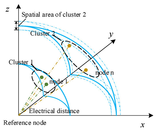
Figure 3.
Cluster regional structure.
Electrical distance is based on voltage and loss-sensitivity-matrix analysis, which is used to measure the coupling closeness of voltage changes between nodes. The output form of DG connected to the distribution network is mainly active power; the 10 kV submarine cable has small geometric distance and close connection and the reactance is smaller than that of the overhead line of the same grade. Therefore, its resistance and reactance are not much different. Therefore, based on the voltage-active power-sensitivity matrix and the loss-sensitivity matrix, the control ability of the active power of node m to the voltage and loss of each node can be expressed by the column vector VSm of the voltage-active power-sensitivity matrix and the column vector LSm of the loss-sensitivity matrix:
In Equation (22), the derivative of the power of each node with respect to node m can be regarded as a dimension of spatial coordinates. Matrix VSm reflects the relationship between voltage and active power and LSm reflects the relationship between loss and active power. The specific solving process of electrical distance is shown in the following equations:
where VSmin and VSmax are the minimum and maximum values of voltage-active power sensitivity matrix elements, respectively; LSmin and LSmax are the minimum and maximum values of loss-sensitivity matrix elements, respectively; xvmk is the k-th spatial coordinate of node m after the normalization of voltage-sensitivity matrix elements; xlm is the spatial coordinate of node m after the normalization of loss-sensitivity matrix elements; dij is the electrical distance between nodes i and j; p and q are the weight coefficients of different indicators; and p + q = 1. Equations (23) and (24) unify the data of voltage sensitivity and loss sensitivity to one standard through minimum–maximum normalization transformation and combined with the Euclidean distance calculation method of Equation (25), the size of the electrical distance between nodes i and j can be solved when the degrees of influence of loss sensitivity and voltage sensitivity are different.
Nodes with relatively close electrical distance have a similar influence of active power on voltage and loss, and these nodes can be grouped into a sub-cluster that can be controlled with one voltage controller. According to Equations (15) and (19), the factors affecting the electrical distance mainly include the impedance of the line, the voltage amplitude of the node, and the injected power of the node.
4. WT/PV ES Optimization Decision
4.1. General Idea
To make full use of the abundant wind and solar resources on the sea, this study proposes a WT/PV ES siting and sizing optimization strategy for offshore oil–gas platforms. The detailed process is shown in Figure 4.
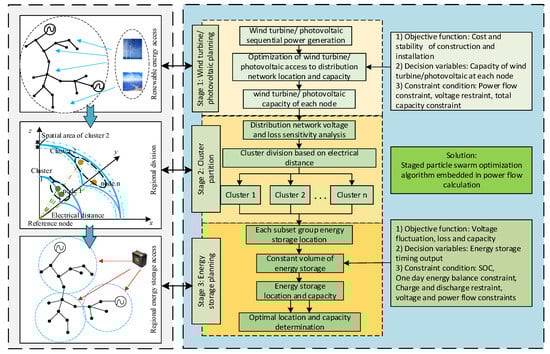
Figure 4.
Hierarchical planning process.
This WT/PV ES planning mode not only considers the static stability of the distribution network, but also takes into account the voltage fluctuation and loss. Therefore, it can effectively improve the stability margin of the distribution network and reduce the impact of uncertainty in wind/solar availability.
4.2. Stage 1: WT/PV Siting and Sizing
In the first stage, the WT/PV capacity planning aims to determine the optimal connected WT and PV capacity of each distribution network node to improve the power-flow stability of the distribution network and minimize the total cost of offshore WT/PV investment.
4.2.1. Objective Function
The objective function of the upper optimal programming is determined by:
- Power-flow voltage stability F1
Reasonable WT/PV connection will improve the voltage distribution of the entire distribution network and enhance the power-flow stability margin of the distribution network. The goal is to maximize the power-flow voltage stability indicator L within a day, as follows:
- 2.
- Total investment cost F2
Considering the initial investment budget of WT/PV and offshore construction, F2 is defined as the total cost of offshore WT/PV investment and construction; that is:
where C1 and C2 are the per-capacity purchase and construction costs of WT and PV units, respectively, and PW and PPV are the installed capacities of WT and PV units, respectively.
4.2.2. Constraint Condition
- Power-flow constraint of distribution network
When the distribution network operates stably, its voltage and power must satisfy the power-flow equations:
where Gij and Bij are the conductance and susceptance, respectively, between nodes i and j and θij is the phase-angle difference between nodes i and j.
- 2.
- Node voltage constraint
To ensure the power quality of the distribution network, according to the relevant regulations, the node voltage of the power-grid system should be within a reasonable range during operation:
where Ui,min and Ui,max are the minimum and maximum allowable values of node voltage deviation, respectively.
- 3.
- Total capacity constraint of WT/PV access
After the WT/PV unit is connected, to avoid curtailment of wind and solar power, the total capacity minus the total load capacity should not exceed the maximum power that the transformer of the upper power grid can bear:
where PDG is the actual capacity of WT/PV connected to the distribution network and PDG,max is the maximal permitted connected capacity of renewable energy.
4.3. Stage 2 and 3: Cluster Partition and ES Siting and Sizing
In the second stage, after the distribution network is connected to the WT/PV system, the whole distribution network is partitioned into several sub-clusters, according to the electrical-distance calculation method. In the third stage, the ES siting is selected, according to the sensitivity analysis; the voltage fluctuation, active-power loss, and capacity are selected as the objective function, and the output time sequence of ES is selected as the decision variable to plan the ES capacity.
4.3.1. Objective Function
The objective function of ES planning is determined by
- Voltage fluctuation f1
After the storage is connected, the voltage of each node is expected to be more stable and the fluctuation with time is small. The node voltage fluctuation is selected as the objective function:
where n is the number of nodes and U1 and Ui,t are the amplitudes of node 1 (slack bus) and node i, respectively, at time t.
- 2.
- Line loss f2
The line loss of the system can be effectively adjusted by adjusting the storage output, and the total line loss is defined as the objective function; that is:
where Pi,t and Qi,t are the active and reactive power injection of node i, respectively, at time t.
- 3.
- Capacity of storage system f3
While considering the voltage fluctuation and loss of ES regulation, the cost of ES unit capacity should also be considered. Therefore, the total ES capacity is selected as an important indicator to measure the economy of ES, and the corresponding objective function can be obtained by examining the maximum charge/discharge capacity and the upper and lower limits of the SOC of ES in a day:
where tj,s is the starting time of continuous charge/discharge of the j-stage ES; tj,e is the end time of continuous charging/discharging of the j-stage ES; Pch/dis,i is the charge/discharge power of the i-th ES period; SOCmax and SOCmin are the upper and lower limits of the SOC of ES, respectively; and Ne is the amount of ES.
4.3.2. Constraint Condition
When connecting ES capacity, it is necessary to consider not only the power-flow constraints and the node voltage constraints, but also the SOC constraints of ES, the one-day energy balance constraints, and the charge/discharge constraints.
- SOC constraint
Overcharge and discharge of stored energy will affect the service life, so its state of charge should not exceed the upper and lower limits during the use of stored energy.
where SOCi,max and SOCi,min are the upper limit and lower limit of the SOC of the i-th ES, respectively.
- 2.
- Charging and discharging constraints of ES
The SOC of the ES refers to the ratio of the remaining capacity of the ES to the rated capacity at a certain time. Its charge and discharge states are shown in Equation (3).
- 3.
- ES energy balance constraint
To meet the requirements of a day’s dispatching operation, it is hoped that the SOC at the beginning of the day and the SOC at the end of the day will be equal; that is:
4.4. Multi-Objective Interactive Decision-Making Model
To optimize each objective and make its synthesis optimal, a multi-objective interactive decision-making model is introduced:
In this model, f1(x), f2(x), and fn(x) are different objectives. The satisfaction function can be obtained by normalizing the optimal solutions f1, min, f2, min, …, fn, min of multiple objectives ξ1, ξ2, …, ξn:
Let ξ(x) = [ξ1 ξ2 … ξn]T be the overall satisfaction function, where ξ1, ξ2, …, ξn are the best expectations of objective function 1,…,n, with a theoretical value of 1. The best expected value of ξ(x) is ξ*(x*) = [ξ*1 ξ*2 … ξ*n]T. To solve the decision vector solution x*, the overall equilibrium decision function f is defined as follows:
The greater the ξ, the smaller the f, and the closer the target is to its optimum value. Therefore, f can achieve the overall balance of multiple objectives, while taking into account the contradictions of all parties. Therefore, it can obtain a satisfactory solution that is acceptable to all parties.
4.5. An Algorithm Based on a PSO Algorithm and Power-Flow Calculation
In this study, two optimization methods of planning are proposed, according to the actual needs and the above-mentioned objectives, and two algorithms based on a PSO algorithm and a power-flow calculation are used to solve them.
4.5.1. Method I: Single-Objective Power-Limited Mode of Gas Turbine
Considering the working condition of traditional gas-turbine power generation, the original gas-turbine output power is reduced by some percentage so that the turbine has a reserve capacity, and renewable energy such as WT/PV ES is incorporated to supply power to the distribution network load. A single-objective algorithm, based on a PSO algorithm and a power flow calculation, is proposed. Its process is as follows.
- Step 1
Initialize the particle swarm in the first stage, as shown in Figure 4. According to the upper layer constraints and the hourly power generation of WT/PV per unit capacity, initialize the particle velocity, the position, the iteration times, and the gas-turbine working condition and substitute them into the fitness function to calculate the power flow and the objective function to obtain the initial individual optimal decision and the initial global optimal decision.
- 2.
- Step 2
Update the particle swarm of the first stage. Update the speed and position of each particle within the constraint range, update the individual optimal decision and the initial global optimal decision, and increase the number of iterations by one.
- 3.
- Step 3
Check the number of iterations. If the set maximum number of iterations is reached, proceed to Step 4; otherwise, return to Step 2 to continue the iterative calculation.
- 4.
- Step 4
Select the site for ES. According to the second stage, as shown in Figure 4, voltage and loss-sensitivity indicators partition the whole distribution network into clusters and determine the locations of ES for each cluster.
- 5.
- Step 5
Initialize the particle swarm in the third stage (the sizing of ES). According to the WT/PV planning results in the first stage, initialize the particle swarm in the third stage and calculate the ES capacity.
- 6.
- Step 6
Update the Stage 3 particle swarm, as shown in Figure 4. Update the velocity and position of each particle within the constraint range and calculate the power flow and the objective function to update the ES capacity. Increase the iteration number by 1 and update the iteration number.
- 7.
- Step 7
Check the number of iterations. If the maximum number of iterations is reached, output the optimal result of WT/PV ES capacity planning; otherwise, return to Step 6 to continue the iteration.
4.5.2. Method II: Multi-Objective Economic-Limited Mode
According to budget of the investment, the Pareto optimality of WT/PV capacity is solved, and the ES capacity is calculated as a fixed percentage of the total WT/PV capacity. A multi-objective PSO algorithm is proposed, which is based on a niche multi-objective PSO algorithm [24] and power-flow calculation. The specific capacity planning process is as follows.
- Step 1
Initialize the first stage particle swarm. Initialize the WT/PV capacity and location and set the size and iterations of the external archive.
- 2.
- Step 2
Initialize the noninferior solution and the global optimum decision. Calculate the power flow and each objective value according to the initial value to obtain the first noninferior solution, then randomly select the individuals in the external archive as the global optimal decision, according to the roulette method proportional to the fitness.
- 3.
- Step 3
Update the first stage particle swarm. Update the WT/PV capacity and location within the constraint range and calculate the power flow and objective function.
- 4.
- Step 4
Update the external archives and the global optimum decision. Update the external archive with the noninferior solution of the current particle. If the number of individuals in the archive reaches the maximum, replace the individuals with the minimum fitness, according to the roulette method in Step 2, and update the global optimal decision. Increase the number of iterations by one.
- 5.
- Step 5
Check the number of iterations. If the maximum number of iterations is reached, output the Pareto optimal solution set; otherwise, return to Step 3 to continue the iteration.
- 6.
- Step 6
Determine ES location and capacity. According to the results of Step 5, partition the distribution network cluster in the second stage, select the ES for the third stage, and obtain the output capacity optimization planning results.
After the above planning, it is necessary to evaluate the planned WT/PV ES using the stability-evaluation indicator and the power-, capacity-, and energy-penetration indicators of renewable energy [25].
5. Example Analysis
5.1. Example Conditions
The 10 kV system of an oilfield in the Bohai Sea of China was analyzed. The system grid consisted of 16 nodes. Node 16 belonged to the 35 kV distribution network and the other 15 nodes were of 10 kV, as shown in Figure 5. The whole system was connected to the higher-level distribution network through submarine cables. The total load of the network was 103.892 MW and the load of the entire oil field hardly changed over time. Under the existing working conditions, among the eight (total) gas turbines, six were designated for use and two for standby, which were able to meet the power-load consumption of the whole oilfield with the output of the higher-level distribution network. The system structure is shown in Figure 5.
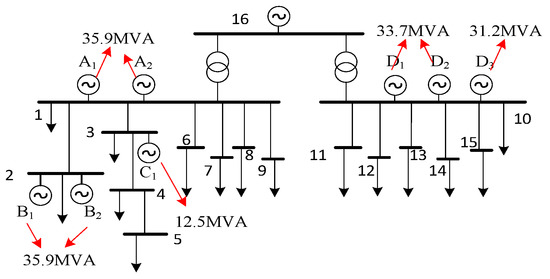
Figure 5.
10 kV distribution network structure.
Based on this topology, this study investigated the rationality of WT/PV ES siting and sizing. Considering the actual demand, Method I and Method II, defined in the previous section, were used to plan the WT/PV ES. Then, comparisons with the original working conditions and analysis were carried out.
5.2. Results and Analysis of Siting and Sizing
5.2.1. Original Working Condition
The eight generators (six for use and two for standby) in the distribution network area were able to meet the load demand with the cooperation of the higher-level distribution network. The load hardly changed with time, and the power flow distribution was relatively stable, as shown in Figure 6.
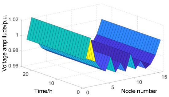
Figure 6.
Power-flow distribution under original condition.
Since the load hardly changed with time, the power flow hardly changed in 1 day when only the gas-turbine output power. The stability indicator F1 was 0.094, the penetration indicator was 0, the voltage fluctuation indicator f1 was 11.96, and the total loss in 1 day was 103.2 MWh.
5.2.2. Scheme I: Power-Limited Mode of Gas Turbine
The output power of the original gas turbine was reduced proportionally and, simultaneously, renewable energy such as wind and solar were incorporated. Considering that the economic and stability indicators were equally important, ξ1(x) and ξ2(x) were each assumed to be 1. When the gas-turbine output decreased by 50%, the optimization curve of the overall WT/PV was as shown in Figure 7. With the increase in the number of iterations, the overall balance decreased, and the optimal scheme which was acceptable to each optimization goal was reached. Considering the different capacities at each node, the WT/PV planning results obtained, based on varying output curves for WT/PV systems, are shown in Figure 8.
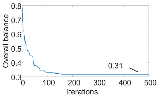
Figure 7.
Iterative curve.
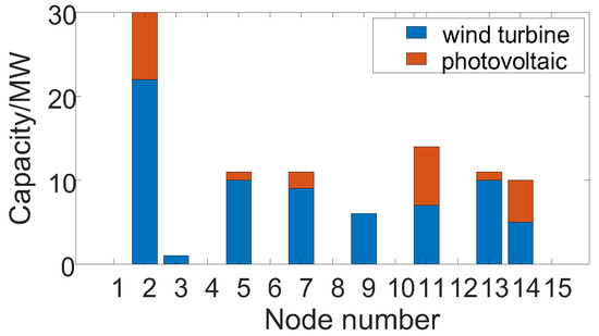
Figure 8.
Wind-turbine and photovoltaic capacity.
The total WT capacity was 70 MW and the total PV capacity was 24 MW. Based on the optimized WT/PV capacity and the predicted output curves, power-flow calculations were performed during each time period. The power-flow distribution result is illustrated in Figure 9, where the x-axis represents the node number, the y-axis represents the per-unit voltage of the node, and the z-axis is the time measured in hours.
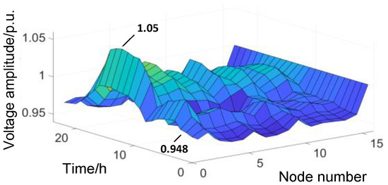
Figure 9.
Power-flow distribution after WT/PV planning.
According to the capacity after WT/PV planning and the load distribution of the distribution network, the second stage of cluster partition was carried out. Based on node 1 and node 10, the electrical distances between nodes 2–9 and 1 and between nodes 11–15 and 10 were calculated. The results are presented in Figure 10, where the x-axis indicates the node number and the y-axis indicates the electrical distance between each node and the reference node.
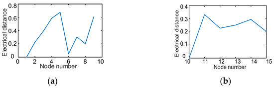
Figure 10.
Electrical distance between nodes: (a) nodes 2–9; (b) nodes 10–15.
Based on the electrical distance between nodes, we grouped together nodes whose electrical distance did not exceed 0.4 and partitioned them into sub-clusters. Nodes 1, 2, 6–8, nodes 3–5, node 9, and nodes 10–15 were partitioned into four sub-clusters, as shown in Figure 11.
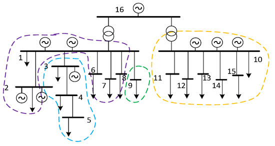
Figure 11.
Cluster-partition results.
According to the cluster-partition results, as well as the internal voltage and loss sensitivity of each sub-cluster, it was decided to connect the ES to nodes 2, 5, and 14. Subsequently, through the optimization algorithm in the third stage, the ES capacities at node 2, 5, and 14 were calculated as 12, 13, and 8 MWh, respectively. Based on the configured energy-storage capacity, we conducted power-flow calculations for each hour to obtain the distribution of power flow, as shown in Figure 12.
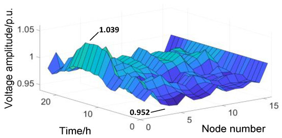
Figure 12.
Distribution of power flow after WT/PV ES planning.
According to the operation state, the power penetration of the system was calculated as 62.80%. Since the load hardly changed, the power penetration and the capacity penetration were always the same. The energy penetration was 39.42% and the stability indicator was 0.057. The maximum values of the node voltage before and after the ES connection were 1.05 and 1.039, respectively, and the minimum values were 0.948 and 0.952, respectively. The fluctuation was significantly reduced. The single-objective optimization process of loss and voltage fluctuation in the total objective is shown in Figure 13. The losses before and after the ES connection were 49.1 MWh and 41 MWh, respectively, and the total voltage fluctuation of all the nodes’ indicators before and after the ES connection were 9.23 and 8.04, respectively. Each objective was optimized through iteration.
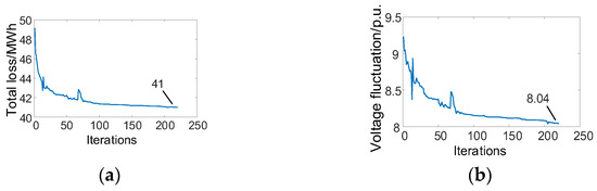
Figure 13.
Distribution of power flow in distribution network with gas-turbine output power reduced by 50%: (a) one-day total loss optimization; (b) voltage-fluctuation optimization.
Using the same methodology, we first performed the siting and sizing of the WT/PV for different scenarios.
The WT/PV planning results obtained when the gas-turbine output power decreased by 30% and 70% are shown in Figure 14.
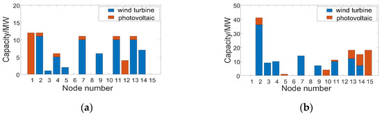
Figure 14.
WT/PV planning results: (a) WT/PV planning results after 30% reduction in gas-turbine output power; (b) WT/PV planning results after 70% reduction in gas-turbine output power.
When the output power of the gas turbine decreased by 30%, the total capacity of WT planned was 62 MW and the total capacity of PV was 21 MW. When the output power of the gas turbine decreased by 70%, the total capacity of WT planned was 105 MW and the total capacity of PV was 43 MW. Similarly, based on the calculation of the electrical distance, we continued to choose nodes 2, 5, and 14 as ES connection points. When the output power of the gas turbine decreased by 30% and 70%, the distribution grid power currents per hour before and after the ES connection were calculated, respectively, and the results are shown in Figure 15 and Figure 16.
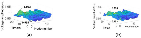
Figure 15.
Distribution of power flow in distribution network with gas-turbine output power reduced by 30%: (a) before ES connection; (b) after ES connection.
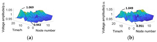
Figure 16.
Distribution of power flow in distribution network with gas-turbine output power reduced by 70%: (a) before ES connection; (b) after ES connection.
When the output power of the gas turbine decreased by 30%, the maximum values of node voltage before and after ES connection were 1.033 and 1.028 p.u., respectively, and the minimum values before and after ES connection were 0.954 and 0.96 p.u., respectively, as shown in Figure 15. The loss decreased from 53.5 MWh to 46.2 MWh and the total voltage fluctuation decreased from 7.58 to 6.17, as shown in Figure 17.
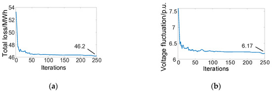
Figure 17.
Optimization of ES connection when the output power of the gas turbine is reduced by 30%: (a) one-day total loss optimization; (b) optimization of total voltage fluctuation of all the nodes.
When the output power of the gas turbine decreased by 70%, before and after ES connection, the maximum values of node voltage were 1.069 and 1.049 p.u., respectively, and the minimum values were 0.942 and 0.951 p.u., respectively, as shown in Figure 16. The loss was reduced from 44.6 MWh to 35.1 MWh and the total voltage fluctuation was reduced from 9.57 to 8.18, as shown in Figure 18.
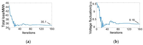
Figure 18.
Optimization of ES connection when the output power of gas turbine is reduced by 70%: (a) one-day total loss optimization; (b) optimization of total voltage fluctuation of all the nodes.
Table 1 presents the results of various indicators before and after the connection of WT/PV ES. When the gas turbine output power decreased by 30%, the planning results of ES capacity were 7.6, 6.1, and 3.3 MWh, the power/capacity penetration was 55.43%, the energy penetration was 34.84%, and the stability indicator was 0.053. When the gas turbine output power decreased by 70%, the ES capacity planning results were 15, 15.2, and 6.3 MWh, the power/capacity penetration was 99.40%, the energy penetration was 61.10%, and the stability indicator was 0.073.

Table 1.
Comparison of various indicators before and after WT/PV ES connection.
It can be seen from the data in Table 1 that, compared with the original working condition, reducing the output power of gas turbine and incorporating renewable energy such as distributed WT/PV ES effectively improved the renewable power, the renewable capacity, and the renewable-energy penetration of the entire oil–gas platform, improved the power flow distribution in the distribution network, and enhanced the static voltage/power-flow stability of the distribution network. Moreover, the addition of WT/PV reduced the active power loss of the system, and the addition of ES in the sub-cluster further reduced the active-power loss and the voltage fluctuation, thereby improving the economy and reliability of the distribution network operation.
5.2.3. Scheme Ⅱ: Economical Customization
According to initial investment budget, when planning WT/PV, considering the economic indicators (in millions of yuan) and stability, the ES is planned to be 30% of the total WT/PV capacity. The multi-objective particle swarm optimization algorithm embedded in the power flow calculation was used to obtain the Pareto optimality-of-economic-and-stability indicator, when the investment budget was limited between RMB 250 million and RMB 350 million (approximately USD 60 million), as shown in Figure 19.
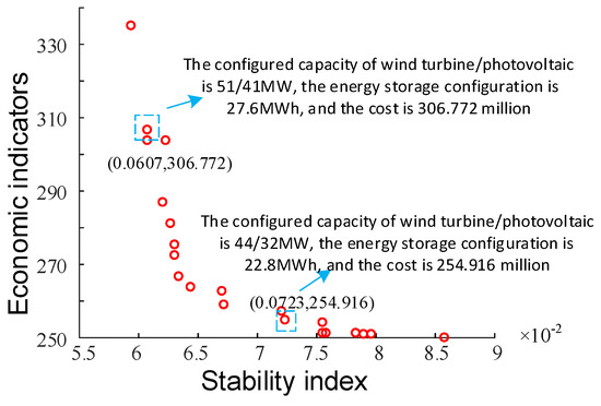
Figure 19.
Multi-objective Pareto optimality.
It can be seen from Figure 19 that when the total WT/PV planning was 92 MW and the total ES planning was 27.6 MWh, the initial investment was RMB 306.772 million and the stability indicator was 0.0607. When the sizing of total WT/PV was 76 MW and the sizing of total ES was 22.8 MWh, the initial investment was RMB 258.607 million and the stability indicator was 0.0723. With the increase in the initial investment, the stability of the distribution network system improved. The sizing optimization results of WT/PV ES were selected according to the weighting of different objectives in the actual scenario.
6. Conclusions
This study proposes a joint planning method of WT/PV ES connected to offshore oil–gas platforms. Based on the power-flow stability indicator, the cluster-partition principle of voltage and loss-sensitivity analysis, and the initial investment, an algorithm based on a PSO algorithm and power-flow calculation was used to solve the two proposed methods. The findings are summarized as follows:
- The optimal planning method of WT/PV ES proposed in this paper can effectively improve the power-flow stability of offshore oil–gas platform distribution networks, improve the penetration of renewable energy, reduce the burden of the distribution network and gas turbines, and improve the economic indicators.
- The cluster-partition principle and the ES connection method proposed in this paper can effectively improve the impact of the uncertainty of WT/PV output power on the distribution network and reduce the distribution network loss and voltage fluctuation.
Through experiments, it was proven that the method proposed in this paper increased the new-energy penetration rate by 55.43–99.4%, reduced the voltage fluctuation by 18.6–35.5%, and reduced the total power loss by 48.2–56.8% by rationally siting and sizing the WT/PV under circumstances in which the output of the gas turbine was reduced by 30–70%. At the same time, after rational siting and sizing for ES, voltage fluctuation was again reduced by 12.9–18.6%, and total power loss was reduced by 13.6–21.3%.
Overall, the WT/PV ES siting and sizing method proposed in this paper can effectively utilize the abundant offshore wind/solar resources, proving the feasibility of offshore large-scale access to decentralized WT/PV power generation projects, which is conducive to the “carbon-neutral” operation of offshore oil–gas platforms in the future.
Author Contributions
Conceptualization, C.H. and C.L.; investigation, C.L.; writing—original draft preparation, J.D.; supervision, C.H. and S.L.; writing—review and editing, J.D. and X.L.; validation, H.L. All authors have read and agreed to the published version of the manuscript.
Funding
The National Key R&D Program of China (2021YFE0103800); the Basic Research Business Fee Project of the Municipal Education Commission (KM201710009002).
Institutional Review Board Statement
Not applicable.
Informed Consent Statement
Not applicable.
Data Availability Statement
Not applicable.
Conflicts of Interest
The authors declare no conflict of interest.
References
- Huang, B.B.; Zhang, Y.Z.; Wang, C.X. Judgment of China’s “14th five-year plan” new energy development and issues needing attention. Electr. Power 2020, 53, 1089–1094. [Google Scholar]
- Jia, T.; Wang, X.Y. Power capacity optimization of multi energy complementary system for offshore platform. Mar. Electr. Electron. Eng. 2017, 37, 55–59. [Google Scholar] [CrossRef]
- Huang, L.L.; Cao, J.L.; Zhang, K.H.; Fu, Y.; Xu, H.L. Status and Prospects on Operation and Maintenance of Offshore Wind Turbines. Proc. Chin. Soc. Electr. Eng. 2016, 36, 729–738. [Google Scholar] [CrossRef]
- Yao, S.G.; Liu, W.; Zhao, Y.H.; Sun, X.F.; Cheng, J. Modeling and Simulation of island / offshore independent photovoltaic power generation system. Ship Eng. 2018, 40 (Suppl. S1), 358–362. [Google Scholar] [CrossRef]
- Yao, G.; Yang, H.M.; Zhou, L.D.; Li, D.D.; Li, C.B.; Wang, J. Development Status and Key Technologies of Large-capacity Offshore Wind Turbines. Autom. Electr. Power Syst. 2021, 45, 33–47. [Google Scholar]
- Sun, Y.S.; Yang, M.; Shi, C.G.; Jia, D.Q.; Pei, W.; Sun, L.J. Analysis of Application Status and Development Trend of Energy Storage. High Volt. Eng. 2020, 46, 80–89. [Google Scholar]
- Moradi, M.H.; Abedini, M.; Hosseinian, S.M. A Combination of Evolutionary Algorithm and Game Theory for Optimal Location and Operation of DG from DG Owner Standpoints. IEEE Trans. Smart Grid 2016, 7, 608–616. [Google Scholar] [CrossRef]
- Li, J.L.; Tan, Y.L.; Wang, H.; Huang, J. Configuration optimization strategy for energy storage system of distribution network and optical storage microgrid. High Volt. Eng. 2022, 48, 1893–1902. [Google Scholar] [CrossRef]
- Ding, M.; Fang, H.; Bi, R.; Liu, X.F.; Pan, J.; Zhang, J.J. Optimal Siting and Sizing of Distributed PV-storage in Distribution Network Based on Cluster Partition. Proc. Chin. Soc. Electr. Eng. 2019, 39, 2187–2201. [Google Scholar] [CrossRef]
- Giannitrapani, A.; Paoletti, S.; Vicino, A.; Zarrilli, D. Optimal Allocation of Energy Storage Systems for Voltage Control in LV Distribution Networks. IEEE Trans. Smart Grid 2017, 8, 2859–2870. [Google Scholar] [CrossRef]
- Ameli, A.; Bahrami, S.; Khazaeli, F.; Haghifam, M. A Multiobjective Particle Swarm Optimization for Sizing and Placement of DGs from DG Owner’sand Distribution Company’s Viewpoints. IEEE Trans. Power Deliv. 2014, 29, 1831–1840. [Google Scholar] [CrossRef]
- Motling, B.; Paul, S.; Dey, S.H.N. Siting and Sizing of DG Unit to Minimize Loss in Distribution Network in the Presence of DG Generated Harmonics. In Proceedings of the 2020 International Conference on Emerging Frontiers in Electrical and Electronic Technologies (ICEFEET), Patna, India, 10–11 July 2020; pp. 1–5. [Google Scholar] [CrossRef]
- Ibrahim, N.N.B.; Jamian, J.J.; Rasid, M.B.M. Penetration Level Limited of Single and Multiple DG Siting and Sizing using PSO Algorithm. In Proceedings of the 2021 3rd International Symposium on Material and Electrical Engineering Conference (ISMEE), Bandung, Indonesia, 10–11 November 2021; pp. 190–195. [Google Scholar] [CrossRef]
- Akbar, M.I.; Kazmi, S.A.A.; Alrumayh, O.; Khan, Z.A.; Altamimi, A.; Malik, M.M. A Novel Hybrid Optimization-Based Algorithm for the Single and Multi-Objective Achievement with Optimal DG Allocations in Distribution Networks. IEEE Access 2022, 10, 25669–25687. [Google Scholar] [CrossRef]
- Yao, Z.; Wu, K.; Zhang, Y.; Yan, Q.; Shi, J.; Sun, J.; Hu, H.; Li, B.; Ye, J. Optimal Allocation and Economic Analysis of Energy Storage Capacity of New Energy Power Stations Considering the Full Life Cycle of Energy Storage. In Proceedings of the 2022 IEEE 6th Conference on Energy Internet and Energy System Integration (EI2), Chengdu, China, 11–13 November 2022; pp. 2592–2599. [Google Scholar] [CrossRef]
- Li, Y.; Lv, Q.; Zhang, Z.; Dong, H. Optimal Allocation of Energy Storage Capacity of Distribution Grid Based on Improved Particle Swarm Optimization Algorithm. In Proceedings of the 2022 3rd International Conference on Advanced Electrical and Energy Systems (AEES), Lanzhou, China, 23–25 September 2022; pp. 291–296. [Google Scholar] [CrossRef]
- Zhao, L.; Zhang, X.; Han, L.; Sun, Y.; Wang, J.; Liu, Z.; Yu, P. Distributed Photovoltaic Generation and Energy Storage Planning of Distribution Network Based on Multi Scenarios. Mod. Electr. Power 2022, 39, 460–468. [Google Scholar] [CrossRef]
- Diamond, K.E. Extreme weather impacts on offshore wind turbines: Lessons learned. Nat. Resour. Environ. 2012, 27, 37. [Google Scholar]
- Li, J.H.; Zuo, J.J.; Wang, S. Risk assessment and analysis of large-scale wind power grid connected power system operation. Power Syst. Technol. 2016, 40, 3503–3513. [Google Scholar] [CrossRef]
- Wen, S.; Lan, H.; Fu, Q.; Yu, D.C.; Zhang, L. Economic allocation for energy storage system considering wind power distribution. IEEE Trans. Power Syst. 2015, 30, 644–652. [Google Scholar] [CrossRef]
- Gao, Y.; He, X.; Ai, Q. Multi Agent Coordinated Optimal Control Strategy for Smart Microgrid Based on Digital Twin Drive. Power Syst. Technol. 2021, 45, 2483–2491. [Google Scholar] [CrossRef]
- Jasmon, G.B. New contingency ranking technique incorporating a voltage stability criterion.IEE Proceedings Generation. Transm. Distrib. 1993, 140, 87–90. [Google Scholar]
- Liu, J.; Bi, P.X.; Dong, H.P. Simplified Analysis and Optimization of Complex Distribution Networks [m]; China Electric Power Press: Beijing, China, 2002. [Google Scholar]
- Liu, W.Y.; Xie, C.; Wen, J.; Wang, J.M.; Wang, W.Z. Optimization of Transmission Network Maintenance Scheduling Based on Niche Multi-objective Particle Swarm Algorithm. Proc. Chin. Soc. Electr. Eng. 2013, 33, 141–148. [Google Scholar] [CrossRef]
- Zhao, B.; Xiao, C.L.; Xu, C.; Zhang, X.S.; Zhou, J.H. Penetration Based Accommodation Capacity Analysis on Distributed Photovoltaic Connection in Regional Distribution Network. Autom. Electr. Power Syst. 2017, 41, 105–111. [Google Scholar]
Disclaimer/Publisher’s Note: The statements, opinions and data contained in all publications are solely those of the individual author(s) and contributor(s) and not of MDPI and/or the editor(s). MDPI and/or the editor(s) disclaim responsibility for any injury to people or property resulting from any ideas, methods, instructions or products referred to in the content. |
© 2023 by the authors. Licensee MDPI, Basel, Switzerland. This article is an open access article distributed under the terms and conditions of the Creative Commons Attribution (CC BY) license (https://creativecommons.org/licenses/by/4.0/).