1. Introduction
Due to the rapid development of semiconductor integrated circuits and digital control technology as well as the many problems existing in traditional airborne actuation systems, more electric aircraft (MEA) technology has become the main trend of modern aviation development. It emphasizes the usage of electric power instead of hydraulic power, pneumatic power, etc.; consequently, it has the advantages of light weight, high power density and efficiency, low cost, simple testing and maintenance, etc. [
1]. At present, the most representative MEA of civil aircraft are Airbus A380 and Boeing 787 aircraft, and that of military aircraft is the F-35 fighter. Airbus A380 and F-35 fighter have already used electro-hydrostatic actuators to drive the primary flight control surface. Boeing 787 aircraft, on the other hand, applies electromechanical actuators (EMAs) to the secondary flight controls, like slat actuators and spoiler actuators [
2]. With the advancement of power-by-wire technology, EMA, which completely abandons the hydraulic system, is bound to have better application prospects. EMA can be divided into two forms according to different driving methods: ball screw EMA with gear reduction mechanism and direct-drive ball screw EMA. The direct-drive EMA, which directly integrates the ball screw pair with the motor in its structure, eliminates the need for a gear reduction mechanism, so it has the advantages of high reliability, high efficiency, and high integration. However, as an emerging technology, achieving the same level of reliability as hydraulic servo systems is challenging for direct-drive EMA, thus limiting its large-scale application [
3]. In order to ensure the safe operation and economic maintenance of aircraft, it is of great significance to accurately and timely diagnose and predict the real-time status of direct-drive EMA.
In recent years, data-driven intelligent fault diagnosis are widely used in the field of fault diagnosis. In most of the existing data-based EMA fault-diagnosis methods, feature extraction and classification are designed and perform separately rather than as a single entirety, so both cannot be optimized simultaneously. For example, dynamic response indicators derived from vibration and current signals of EMA can be utilized as classification features [
4,
5]. Mode decomposition [
6] and information entropy [
7] are also used to constitute the feature vector of EMA. Additionally, principal component analysis (PCA) is often used for the selection and fusion of EMA fault features [
8,
9]. After selecting the appropriate features, these features are fed into a classifier, such as BP neural network, support vector machine, and random forest, for fault classification [
10,
11]. The features of the aforementioned traditional data-based methods usually rely on manual design, requiring certain signal processing technology and diagnostic expertise, which can be unreliable and time-consuming. Moreover, they are mostly used in specific fields and cannot be updated online with changes in application equipment or fields. To address the defects of traditional fault-diagnosis approaches, deep learning methods such as stacked denoising autoencoder, deep belief network, and convolutional neural network (CNN) [
12,
13] have demonstrated great vitality in these years. Unlike traditional methods, deep learning can directly learn the effective fault features adaptively from monitoring signals and perform the fault classification at the same time, thereby achieving end-to-end fault diagnosis. Particularly, the CNN has achieved superior performance in various fault-diagnosis tasks [
14,
15,
16] due to its features of weight sharing, local connection, and multiple convolution kernels. The superior performance of one-dimensional CNN (1DCNN) in the EMA fault-diagnosis problem compared to traditional data-based methods has been demonstrated in prior work [
17]. Therefore, this paper aims to develop a CNN-based intelligent fault-diagnosis model for EMA.
Due to the interaction between the subsystems of fault-identification objects, the fault signals usually appear in multi-scale form. Therefore, conventional CNN methods, which only contain single-scale convolution kernels, may ignore the fault-related information. To address the challenge, several multi-scale network structures have been proposed and have achieved impressive performance. Introducing multi-scale transformation into conventional CNN can enable the network to acquire features of different receptive fields at the same level and improve the diversity and complementarity of fault-related features. For example, Jiang et al. [
18] proposed a multi-scale convolutional neural network structure that can effectively extract multi-scale high-level features. The method was verified on a WT gearbox. Liu et al. [
19] proposed a multiscale kernel CNN to capture the patterns of motor faults. Peng et al. [
20] used a similar multi-branch structure in the feature learning process.
Despite the good performance, those multi-scale CNNs mentioned above simply combine the captured multi-scale features without taking into account differences in the importance of different branches. Therefore, the information related to the fault may not be used effectively, especially in the case of noise interference and load variation. In this paper, the fault-diagnosis object EMA often needs to operate under complex working conditions, such as the complexity and variability of work tasks, the non-linearity and non-stationarity of the signal caused by changes in speed and load, as well as strong environmental noise. To reduce the influence of the above factors, it is required that the intelligent diagnosis algorithm has better adaptability and can reduce the sensitivity to various uncertainty sources. In recent years, attention mechanisms have been widely utilized to achieve efficient resource allocation and information-capture capability of models for intelligent fault diagnosis [
21], natural language processing, machine vision, and the broader fields of deep learning [
22,
23]. Li et al. [
24] demonstrated the effectiveness of attention mechanisms in bearing intelligent fault diagnosis by locating input data segments and visualizing network-learned diagnosis knowledge. Ding et al. [
25] proposed a wind turbine blade intelligent anomaly-detection method based on attention mechanism, which solves the memory occupancy problem of the input sequence and improves the accuracy of anomaly detection. Kong et al. [
26] proposed an attentional recursive autoencoder hybrid model classification algorithm for the early fault diagnosis of rotating machinery. The network is able to extract the most valuable features from the input signal.
In order to make the network fully capture the fault-related features at different scales and levels and reduce sensitivity to various sources of uncertainty, a multi-scale feature fusion CNN (MSFFCNN) is herein proposed to diagnose EMA faults. The multi-scale network structure is applied to EMA fault diagnosis for the first time. Moreover, unlike the aforementioned multi-scale methods, an attention mechanism module is used. Firstly, the attention module enables effective recalibration of feature channels, enhancing essential features and suppressing invalid ones. This improves the model’s ability to focus on the most relevant information. Secondly, it further recalibrates features learned by each branch and multiscale fusion features, aiming to aggregate the optimal multiscale features. This results in improved feature representation and better model performance. To verify the performance of the proposed algorithm, an EMA system experimental platform was built, and the fault injection experiment was carried out for several common faults. The collected data were used to train and test the proposed method compared with the state-of-the-art algorithms, especially under variable load and noise conditions. This paper is organized as follows.
Section 2 describes the structure of the direct-drive EMA and introduces its common faults.
Section 3 details the proposed MSFFCNN for EMA fault diagnosis.
Section 4 details different experiments to verify the effectiveness and superiority of the MSFFCNN.
Section 5 summarizes this paper.
2. Structure and Faults Analysis of the Direct-Drive EMA
2.1. Structure of the Direct-Drive EMA
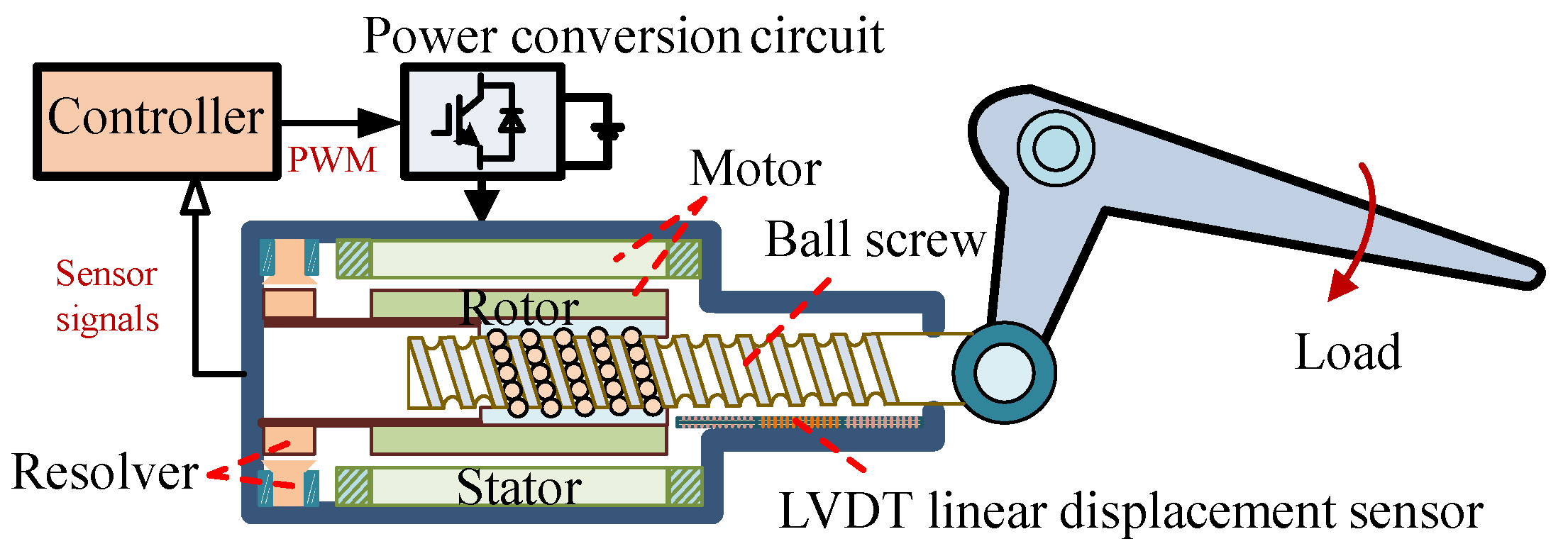
The actuator is essentially a position servo control system, which drives the load by controlling the operation of the motor to achieve the target position control. The difference between EMA and other actuators is that there is only one type of energy transmission in the electromechanical actuation system, and mechanical transmission is used instead of hydraulic transmission. The structure of the direct-drive EMA is shown in
Figure 1. It is mainly composed of a controller, power conversion circuit, motor, ball screw, and load and feedback components (current sensor, resolver, and LVDT linear displacement sensor).
Among them, the motor adopts a switched reluctance motor (SRM) with a certain fault tolerance and is matched with a direct-drive structure that cancels the gearbox, which greatly improves the reliability of EMA. When the EMA works, the controller controls the power converter by processing the flight commands as well as the feedback sensor signals, and the switching signals generated by the power converter control the motor rotation. The ball screw then converts the rotational motion of the rotor into a straight-line motion, which drives the swing of the aircraft control surface. In the whole process, the real-time measured position, velocity, and current information are fed back to the controller by the current sensor, i.e., the rotary transformer and the linear variable differential transformer (LVDT) so as to realize the closed-loop control.
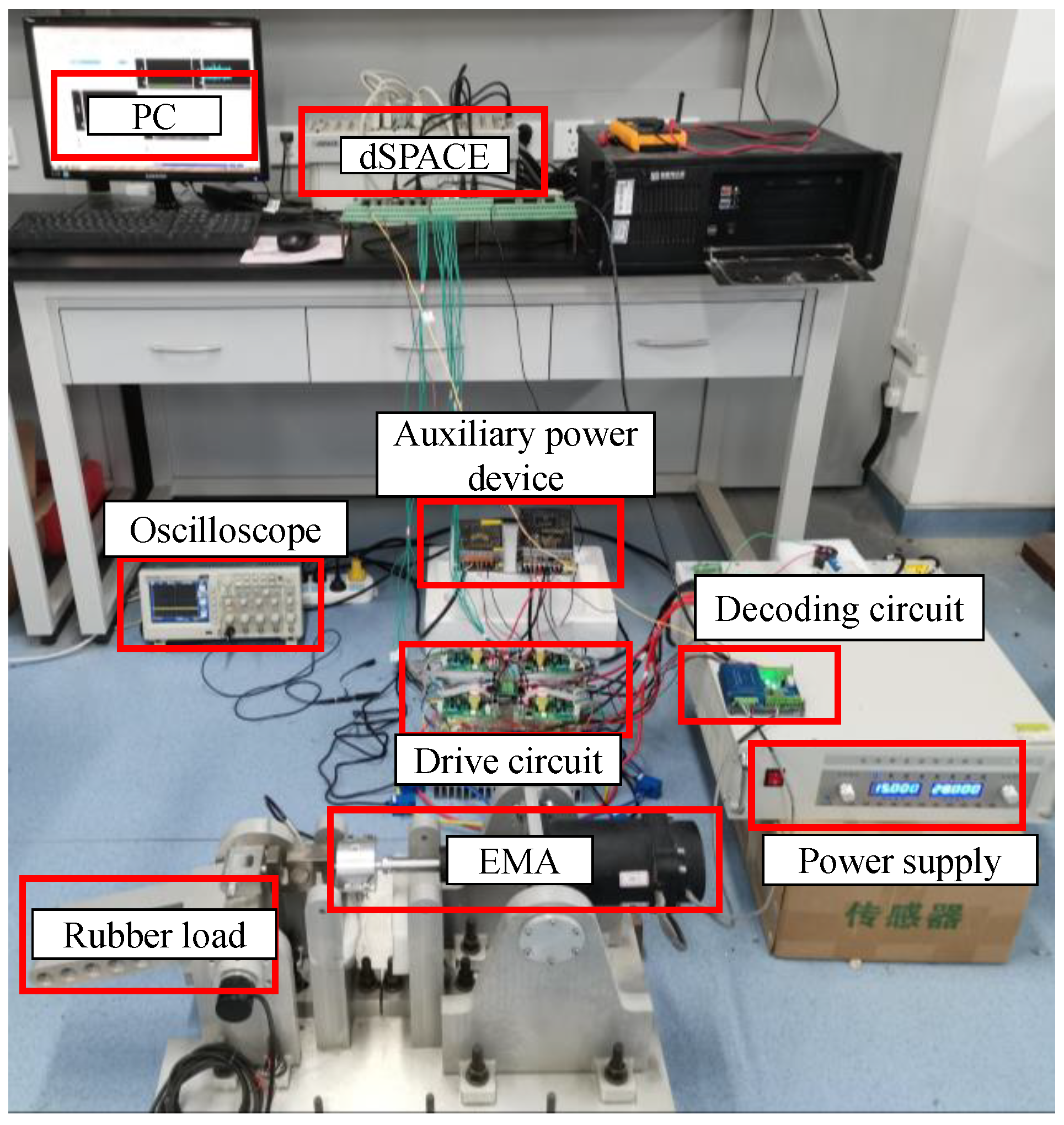
This study built an dSPACE-based EMA system experimental platform, as shown in the
Figure 2. The experimental platform is composed of PC, dSPACE, auxiliary power supply, IGBT drive circuit, rotary decoding circuit, power supply, EMA, load rudder, sensors, and oscilloscope. The dSPACE hardware platform is mainly used to provide a real-time control platform for semi-real objects. In this experiment, DS1103PPC was used to output 8 PWM motor control signals through the digital I/O port of the main processor to control the opening and closing of IGBT. The SRM current analog signal output by the Hall sensor and the LVDT position signal output by the decoder board are collected by the ADC module. In addition, through the incremental encoder interface, the rotary signal of the motor can be directly input to the DS1103PPC through the rotary decoding board so as to be used for the measurement of the motor position and speed.
2.2. Fault Categories and Data Processing
From the perspective of the composition of EMA, there are four types of failures that may occur during operation: motor failure, electrical failure, mechanical failure, and sensor failure. Due to the harshness of the actual application conditions of EMA, such as overload, harsh environment, lubrication problems, and manufacturing defects, it is prone to mechanical failures. Furthermore, as a key component of the drive servo actuation system, the motor usually runs at a higher speed, accompanied by temperature rise in the housing and obvious mechanical stress, so the motor is prone to a winding short circuit and rotor-shaft eccentricity. Electrical faults mainly refer to faults in EMA’s power supply and controller and sensor faults.
This paper comprehensively considers the three factors of EMA fault-occurrence frequency, degree of influence, and similarity of fault performance. The four faults of motor winding turn-to-turn short circuit, ball screw wear and jam, IGBT open circuit, and sensor deviation were selected for research. The specific experimental data and status labels are shown in
Table 1. Among them, after the faults have been determined, the IGBT open circuit and the winding turns short circuit can be specific to the fault of a certain phase or a few phases according to the value of each phase’s current sensor.
Taking the IGBT fault as an example, the open-circuit fault of IGBT is simulated by setting the driving signal of the IGBT to low at a certain time.
Figure 3 shows the current and position signals of EMA before and after the fault. It can be seen that the fault-phase current of IGBT fault increases rapidly, and the position response is slightly deviated from that before the fault, which affects the performance of the EMA system.
Under different fault conditions of EMA, the four-phase current signal output of EMA is collected at the sampling frequency of 10 kHz, and then, the sum of the four-phase current constitutes a signal.
Figure 4 shows an example of the combined signals in five states, all of which have been normalized.
In order to facilitate the training of the convolutional neural network and reduce the interference of different working conditions on the model, each segment of the signal x is normalized. The size of the data is an important factor of the success of deep learning. Generally speaking, the more training samples of a network model, the better its generalization performance. Therefore, in the process of deep learning model training, data augmentation technology is often used; that is, without a substantial increase in data, limited data can generate value equivalent to more data. Taking into account that the output of the electromechanical actuator is a one-dimensional sequence signal, this paper adopts the overlapping sampling method to achieve the purpose of data amplification. The sampling method is shown in
Figure 5.
The above combined signals are segmented with a certain overlap ratio so that the training set, verification set, and test set are obtained. The specific methods are as follows:
where
m is the maximum number of divisible samples of each signal segment;
L is the length of each signal;
l is the set sample length;
λ is the overlap rate;
xi′ is the
i-th data sample after segmentation,
i ∈ [1,
m];
x′ is the normalized signal.
In this study, the sample length l = 4096 and the signal with L = 180,000 were divided with overlap rate λ = 1/3 to achieve sample-set amplification, resulting in a set of 6144 samples. From this set, 800 samples were randomly selected for each state as the training set, while 200 samples were reserved for validation, and 24 samples were used for test. The validation set can be utilized to monitor the occurrence of overfitting during model training. Typically, when the validation set’s performance stabilizes, further training will cause the training set’s performance to continue to improve, while the validation set’s performance will plateau or even decline, indicating overfitting. All model accuracy tests were conducted solely on the test set to evaluate its generalization ability and ensure the reliability of the final results.
3. Proposed MSFFCNN-Based Fault-Diagnosis Method
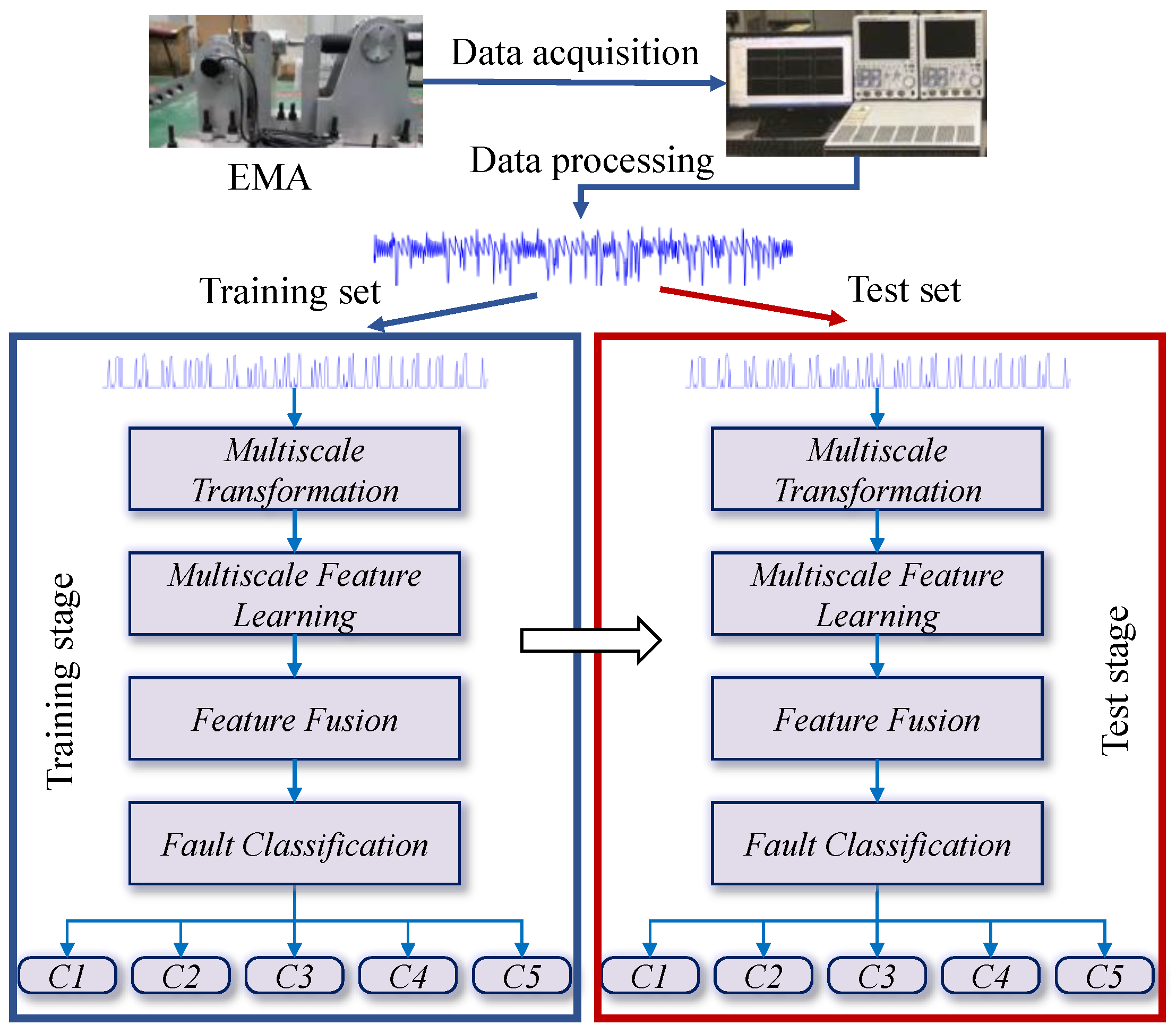
The MSFFCNN is designed for fault diagnosis of EMA, which consists of four sequential stages: multi-scale transformation, feature learning, feature fusion, and fault classification. The overall process of the fault-diagnosis system is shown in the
Figure 6.
3.1. Multiscale Transformation
The so-called multi-scale is actually the sampling of different granularities of the signal. Typically, different features can be observed at different scales to complete different tasks. The multi-scale transformation stage in this paper adopts a parallel multi-branch topology. For a given 1-D signal
x (
), multiple consecutive signals {
y(
k)} with different granularities are constructed by a simple process of down-sampling. The representation method of multi-scale down-sampling is shown in
Figure 7, and its mathematical description is as follows:
where
k is the length of the non-overlapping window in down-sampling (also called the scale factor), and multiple filtered signals with different scales, respectively (i.e., scale1, scale2, and scale3) can be obtained. Typically, the size of
k is related to the details and trends of feature learning later.
Following
Figure 7, the original signal was sampled on three different scales to feed into the trunk and branch module (TBM) in the multi-scale feature learning stage.
3.2. Multiscale Transformation
After obtaining three granular signals with different scales, each granular signal {
y(k)} (
k = 1, 2, 4) will be fed into the TBM separately to learn useful and advanced features. As shown in
Figure 8, each TBM consists of three sets of alternately stacked convolution layers and max-pooling layers.
The signals pass through three pairs of stacked convolutional layers in parallel (C1(k), C2(k), and C3(k)) and pooling layers (P1(k), P2(k), and P3(k)), learning in an advanced and effective way from multiple granular signals of different time scales’ fault characteristics. Specifically, each granular signal uses filters (convolution kernels) of different sizes so that each parallel convolutional layer at the same level can obtain the characteristics of different receptive fields and enhance its capture range of high- and low-frequency features taking into account the overall details of the input signal, thereby improving the diagnostic performance of the model.
The first convolutional layers (C1
(1), C1
(2), and C1
(4)) have signal lengths of
N,
N/2, and
N/4, respectively. For each first convolution, the size
m of the corresponding convolution kernel decreases as the value of
k increases, which is beneficial to better extracting useful features. Taking the
i-th element
ai of the
j-th output feature map
aj of the first convolutional layer ((C1
(k)) as an example, the following is obtained:
Among them, w is the weight vector of the j-th convolution kernel; b is the bias term; yi:i+m−1 is the m-length sub-signal of the input signal y starting from the i-th time step; σ(·) is a nonlinear activation function, namely the rectified linear unit (ReLU); s is the moving stride of the j-th convolution kernel on the signal y.
In order to increase the sparsity of the model and improve the speed of network training, maximum pooling is used to perform nonlinear down-sampling of the input feature map. Its advantage is that position-independent features can be obtained. Suppose that one input feature map is traversed with the pooling step size
w, and one can be calculated for each sliding step
w. For the corresponding local maximum
pj, there will be (
L-
m)/
ws + 1 local maximum at the end of the traversal and will finally constitute the feature map
pt output by the maximum pooling layer (P1
(k)). The specific mathematical formulas are as follows:
For each granular signal {
y(k)} after C1
(k) and P1
(k), a certain number of new feature maps are generated. Then, these feature maps are used as the input of C2
(k), and the same operations in Equations (3)–(6) are repeated, outputting a new feature map. Similarly, assuming that
K convolution kernels are used in C3
(k), the output of the max-pooling layer (P3
(k)) is
K new feature maps, and take
q(k) as the concatenation result of the corresponding feature maps obtained after each granularity signal {
y(k)} through the above process, formalized as follows:
Finally, the feature representation
q(k) output after each granularity signal {
y(k)} undergoes continuous feature learning is flattened into a one-dimensional feature vector
q. Since the scale factor
k = 1, 2, 4 is selected in this paper, vector
q can be represented by the following:
It can be seen from (8) that the final feature representation q has three different scales. Therefore, compared with the traditional single-scale representation, multi-scale feature learning has a larger feature-capture range, which is conducive to extracting rich and complementary features. The characteristics of the system provide a better distinguishing effect for the next step of fault classification.
3.3. Feature Fusion
Multi-scale feature learning realizes simple concatenations of different scale features. However, it cannot represent the difference in the importance of features. Therefore, an effective feature fusion mechanism is needed.
In this paper, an attention mechanism module is used after the feature fusion layer to distribute the weight of multi-scale feature channels. The network can selectively strengthen the useful features for fault identification and suppress invalid or even wrong information. The structure of the efficient channel attention module is shown in
Figure 9.
Assume that the input feature graph of the attention module is
, where
W and
C are size and channel dimension of the feature graph. By using global average pooling
FAvg to compress information of the feature graph
Y, the channel statistical vector
z is obtained:
After that, two fast one-dimensional convolutions are used to self-adaptively encode the channel correlation. The importance of different channels is quantified by activating function σ, thus generating the weight vector
z′ of channels. The mathematical description of this process is shown as follows:
where
Fconv is the convolution operation using the convolution kernel of 1 × k and channel vector
z;
F′
conv is the convolution operation using the convolution kernel of 1 × k and vector after
Fconv;
and
are the ReLU function and Sigmoid function, respectively.
By multiplying the input feature graph Y and the weight vector z′ of the channel, the calibrated feature graph Y′ of the channel can be obtained:
where
zi′ represents the importance of the corresponding channel.
In order to prevent network degradation and improve its generalization performance, a residual connection is added after channel calibration; thus, the output of the attention mechanism module is Y″ = Y + Y′.
3.4. Fault Classification
A combination of a fully connected hidden layer and a softmax layer is used to perform classification. The specific method is to first use dropout on the one-dimensional feature vector
q obtained in the previous stage and use it as the input of the fully connected layer. The hidden layer uses ReLU as the activation function, and the softmax function is used in the output layer. In this paper,
Y represents the category label of EMA’s health status. Suppose it has
n categories; that is, given an input sample
x, the probability that sample
x belongs to category
c is given:
where
is the parameter that needs to be learned in the model;
is the normalized function, and
is the normalized function.
For any given input sample, MSFFCNN will predict a result, but it is hoped that the predicted value of the model is as consistent as possible with the true value. In order to achieve this goal, it is necessary to minimize the distance between the predicted value and the true value, which is the role of the loss function:
where
m is the number of samples or the input batch size;
I{·} is the index function, and when the
I{·} value is true, the index function value is 1; otherwise, the index function value is 0.
In order to minimize the loss function value of the model, it is necessary to optimize and adjust the weight of the neural network, and the optimizer uses the back-propagation algorithm to complete it:
where
θ* is the optimal parameter of the model;
L (·) is the loss function;
f (·) and
y are the output value and target value of the model, respectively.
3.5. Visualization Analysis of MSFFCNN
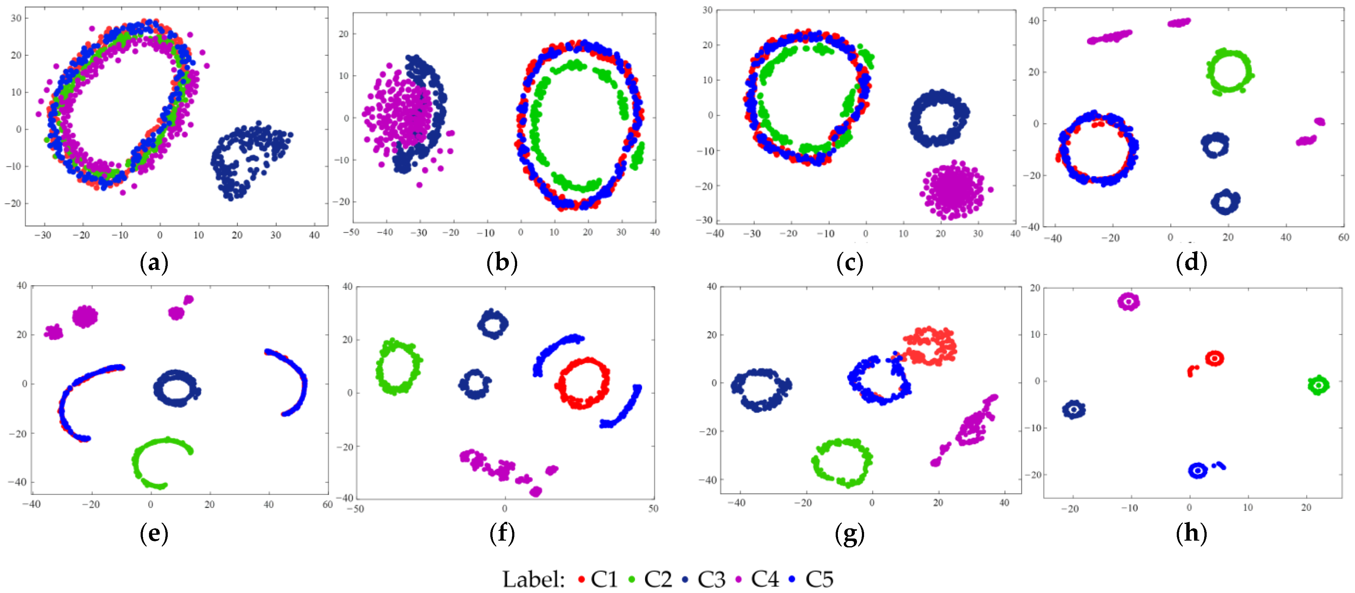
In order to show the classification process of the MSFFCNN, the t-SNE technology is used to visualize half of the samples in the test set. Due to the large number of network layers, only the two-dimensional distribution under one branch is shown here, as shown in
Figure 10.
As can be seen from
Figure 10, samples of various categories of the original signal are jumbled together and completely indistinguishable. With the increase of the convolutional layers, all categories of originally linearly indivisible samples can be almost distinguished in the feature fusion layer and completely distinguishable in the softmax layer, which indicates that the nonlinear representation ability of the MSFFCNN is gradually enhanced. In the softmax layer, all samples are kept very far apart from each other to avoid the occurrence of wrong classification, which indicates that the model has good robustness.


 ,
, 


