Article

Research on Wind Power Prediction Based on a Gated Transformer

1
Faculty of Applied Sciences, Macao Polytechnic University, Macao, China
2
New Energy and Power System Research Center, Ningbo Polytechnic, Ningbo 315806, China
3
Macao Polytechnic Institute, Macao, China
*
Author to whom correspondence should be addressed.
Appl. Sci. 2023, 13(14), 8350; https://doi.org/10.3390/app13148350
Submission received: 25 June 2023 / Revised: 12 July 2023 / Accepted: 12 July 2023 / Published: 19 July 2023

Abstract

:
Wind power, as a type of renewable energy, has received widespread attention from domestic and foreign experts. Although it has the advantages of cleanliness and low pollution, its strong randomness and volatility can bring disadvantages to the stable operation of the power grid. Accurate power prediction can avoid the adverse effects of wind power, and is of great significance for power grid frequency regulation, peak shaving, and energy improvement. However, traditional wind power prediction methods can only achieve accurate predictions in the short term and perform poorly in medium- to long-term prediction tasks. To address this issue, a power prediction model based on a Gated Transformer is proposed in this paper. Firstly, it can extract features from different types of data sources, effectively capture their correlations, and achieve data fusion. Secondly, gating unit, dilated convolution unit, and multi-head attention mechanism are added to improve the Receptive field and generalization ability of the model. In addition, adding a decoder to guide data prediction further improves the accuracy of prediction. Finally, experiments are carried out with the data collected from typical wind farms. The results show that the proposed Gated Transformer achieves consistent state-of-the-art results in prediction tasks on different time scales.

1. Introduction

Compared with traditional fossil fuels, new energy technologies, including wind energy, have the advantages of zero emissions, viability, and abundant reserves. In recent years, wind power generation has enjoyed great popularity both at home and abroad, as a result of the continuous progress in the maturity of its related application technology [1,2]. However, there are still some limitations in wind resources. Its unique strong volatility and randomness affects the stability of power systems [3]. In particular, the reduction in the proportion of traditional power generation, such as firepower and hydropower, brings about the reduction in frequency modulation and voltage regulation ability of power systems [4]. Fluctuations in the load side resulting from shifts in demand can lead to a decrease in both system voltage and frequency due to weakened stability. In more severe scenarios, this can escalate to cause disconnection of the system and subsequent power failure. Therefore, it is necessary to reduce the impact of volatility on the system while steadily increasing the proportion of wind power generation [5,6]. The main importance of high-precision power prediction lies in (1) Economic dispatch—optimizing the output of conventional units based on the predicted output curve of the wind farm, in order to reduce operating costs; (2) Enhancing the safety, reliability, and controllability of the system based on the variation pattern of wind power output; (3) Optimizing the value of electricity in the electricity market. In the electricity market, wind farms predict wind power and participate in bidding in the electricity market. The power grid company predicts the power of wind power to ensure the safe and economic operation of the system.
Wind power prediction is mainly divided into short-term series prediction and medium–long-term series prediction [7]. Taking the time resolution of 15 min as an example, the short-term mode mainly predicts the wind power changes in the next few hours, while the medium–long-term mode predicts the wind power changes in the next few days [8]. Wind power prediction methods are mainly composed of physical methods, mathematical methods, and artificial intelligence methods. Physical methods use the aerodynamic factors of terrain and weather to establish the corresponding physical model, combining the real-time weather information [9,10,11]. Although this method has the highest accuracy in theory, its high complexity and poor robustness limit its application in practical engineering. Mathematical methods mainly use mathematical statistical tools to make mathematical analysis and regression predictions of collected data [12,13]. However, this approach lacks universality, as it only attains average levels of accuracy and heavily relies on mathematical computations. With the rise of deep learning, artificial intelligence prediction methods based on neural network have attracted the attention of experts worldwide. The introduction and deployment of smart grid technology facilitate the acquisition of vast quantities of data and information. The abundance of such data ensures the accuracy and generalizability of artificial intelligence methodologies [14,15].
Relying on a large number of network structures, deep learning is designed to conduct deep feature mining on historical data, find out hidden and universal key information, and then realize prediction through feature decoding [16]. Reference [17] used Arima for wind power prediction. It has the advantages of simple structure and easy fitting, but it has difficulties in dealing with non-stationary stochastic process. Moreover, this method has poor performance in handling multi-feature data sources. Reference [18] used Variational Modal Decomposition (VMD) to decompose wind power into fluctuating and random components, reducing the randomness of power, and uses Long Short-Term Memory (LSTM) for power prediction separately. Although good results have been achieved in short-term forecasting, when confronted with the long-term prediction task, significant computational burdens arise, making it susceptible to memory decay or forgetting. Reference [19] utilized an attention mechanism to avoid feature loss in the encoding process of the LTSTM algorithm. However, the information from multi-feature data sources is not fully utilized, and there is still the limitation of Receptive field. In addition, this method does not address the drawbacks of memory decline in medium–long-term prediction tasks. Reference [20] improved the power prediction accuracy through Feature engineering technology and a gradient lifting tree algorithm based on the Numerical Weather Prediction (NWP) system. Although this method can utilize NWP-related data, it cannot achieve efficient feature mining. The lack of attention mechanism also makes it difficult for the model to converge. Reference [21] considered wind speed correlation and used Gaussian regression for data correction to achieve power prediction. Although this can improve the accuracy of prediction, there are drawbacks such as high computational complexity, high sampling requirements, and difficulty in parameter selection. Reference [22] used fusion models for multi-model prediction using the Stacking framework. This method only integrates multiple models with weights and lacks theoretical innovation. In addition, Data breach and over fitting are serious problems in cross-training.
In summary, traditional prediction models are limited by the strong randomness and volatility in the data themselves, which results in poor performance in medium- to long-term wind power prediction tasks. Based on the above motivations, we propose a prediction model based on a Gated Transformer. In Section 2, data analysis and processing is completed. The results qualitatively verify the low correlation in wind history data and the feasibility of introducing NWP data. Section 3 introduces three basic unit model structures, which lay the foundation for model optimization based on traditional Transformers. By redesigning the model structure, feature extraction and fusion of different data sources can be achieved. Then, multiple units are connected in series through Feature selection to ensure the efficiency of feature processing and ensure that the model can effectively capture the changes in data within and between cycles. Section 5 is an experimental section that quantitatively verifies the feasibility and superiority of the proposed scheme. Our contributions are summarized in three points:
(1) Comparative analysis and feature mining of wind power data have provided qualitative and quantitative judgments on the dataset itself. The data correlation in wind power itself is relatively low, making it unsuitable for traditional neural network models. NWP data are highly correlated with wind power data, which can be added as auxiliary information to help the model realize power prediction;
(2) The traditional Transformer framework has been optimized. Gating unit, dilated convolution unit, and multi-head attention mechanism are added to improve the Receptive field and generalization ability of the model. In addition, adding guidance information to the Decoder input unit further improves the prediction accuracy of the model;
(3) Experiments are carried out with the data collected from typical wind farms. The results show that the proposed Gated Transformer achieves consistent state-of-the-art results in prediction tasks on different time scales.

2. Data Analysis and Preprocessing

2.1. Analysis of Wind Power Characteristics

2.1.1. Comparison of Different Data Sources

Wind power prediction is essentially a kind of time series prediction. The deep learning network for time series prediction can be applied as a model to wind power prediction [23,24,25]. However, the spatiotemporal correlation and characteristics of the data source itself are one of the important factors that affect the predictive performance of the model, and can also have a significant impact on the selection and design of the model. Therefore, it is necessary to study the characteristics of the data themselves. There are many types of time series data, involving multiple fields such as stocks, electricity, healthcare, and transportation. This paper selected the classic power-related datasets Electrical Transformer Temperature (ETT) and Electricity and Wind Power datasets for feature comparison.
ETT: It aims to predict the future oil temperature of power transformers, which is a critical indicator in electric power long-term deployment. It includes two-year data from two separate counties in China. To explore the granularity problem, data collection was conducted at a sampling frequency of 15 min and 1 h, respectively, to form ETTh and ETTm datasets. The data for each time step are composed of target oil temperature and six power load characteristics.
Electricity: The Electricity dataset is designed to predict future power loads and is an important reference factor for long-term planning of power systems. It includes the electricity load of 321 different types of customers for 2 years. The sampling period is in hours, and the load unit is kWh.
Wind Power: The wind power dataset is the main dataset studied in this paper, which aims to predict the change in wind power in the future and help the power grid to complete power planning. It includes output data from a total of 20 wind farms within 2 years, as well as auxiliary information such as wind speed, temperature, pressure, humidity, etc. The sampling period is 15 min, and the power unit is MW.
In order to visually observe the characteristics of the data themselves and facilitate comparison, all data sources were standardized by Z-Score method, setting the sampling period to 1 h and the sampling duration to 1 week. The comparison of data waveforms is in Figure 1a. It can be seen that the period of ETT data is long with slow change, and there is basically no violent fluctuation. The Electricity data exhibit significant periodicity and short-term repeatability. This is because there is a strong correlation between electricity load and electricity usage time. During the day, the electricity load is high, while, at night, the electricity load is low and cyclic. Unlike the two classic datasets mentioned above, wind power data have their own unique characteristics. The fluctuations are large and irregular. In the early stage, the power value is very small, but in the later stage, it rapidly increases, and, after maintaining it for a period of time, it quickly drops back. This phenomenon is also known as wind power climbing. This is because wind power is strongly correlated with wind resources, and wind itself has irregularity and volatility. Such data features may also result in better short-term predictions, but they can pose challenges to medium–long-term predictions.

2.1.2. Analysis of Different Time Scales

Due to the fact that the sampling waveform in the previous text is only one week of data, there may be some specificity. In Figure 1, the data characteristics in the time dimensions of year, season, month, and week can be observed. After the same standardization process, we drew European standard fluctuation charts for different time periods, as shown in Figure 1b. It can be seen that, when observed on a weekly basis, the wind power shows a climbing phenomenon on the 5th to 6th days, while other time periods have very small values with occasional slight fluctuations. When observed on a monthly basis, it can be seen that the frequency of climbing phenomena is relatively low and there is no specific pattern. When observed quarterly and annually, it is found that this characteristic runs throughout the year and is not affected by quarters and months. It can be seen that wind power presents high volatility and randomness throughout the year, and it is difficult to find its regular characteristics. In a short time period, the peak–valley characteristics of the data are obvious, and the wind power is low at most times. When the wind blows, the power increases rapidly, and, after a period of time, it quickly falls back. This characteristic is different from the long-term stability of and short-term regular fluctuation in classical time series. Therefore, it is necessary to mine and analyze the features of this unstable data source.

2.2. Correlation Analysis of Historical Data

As mentioned earlier, the wind power waveform can be observed to have strong volatility and randomness. Such data features pose difficulties for power prediction. This is because the conventional prediction algorithms for time series data sources typically involve analyzing and extracting historical data characteristics, transferring them to a neural network for computation, and ultimately achieving series prediction through regression techniques [26,27]. However, such algorithms have high requirements for the correlation in historical data. Furthermore, the data characteristics of strong randomness and volatility are inevitable, which leads to the low correlation between the future changes in data and historical data in a long time scale, which seriously affects the accuracy of the prediction model. In order to verify this assumption, this paper analyzes the correlation in the data.
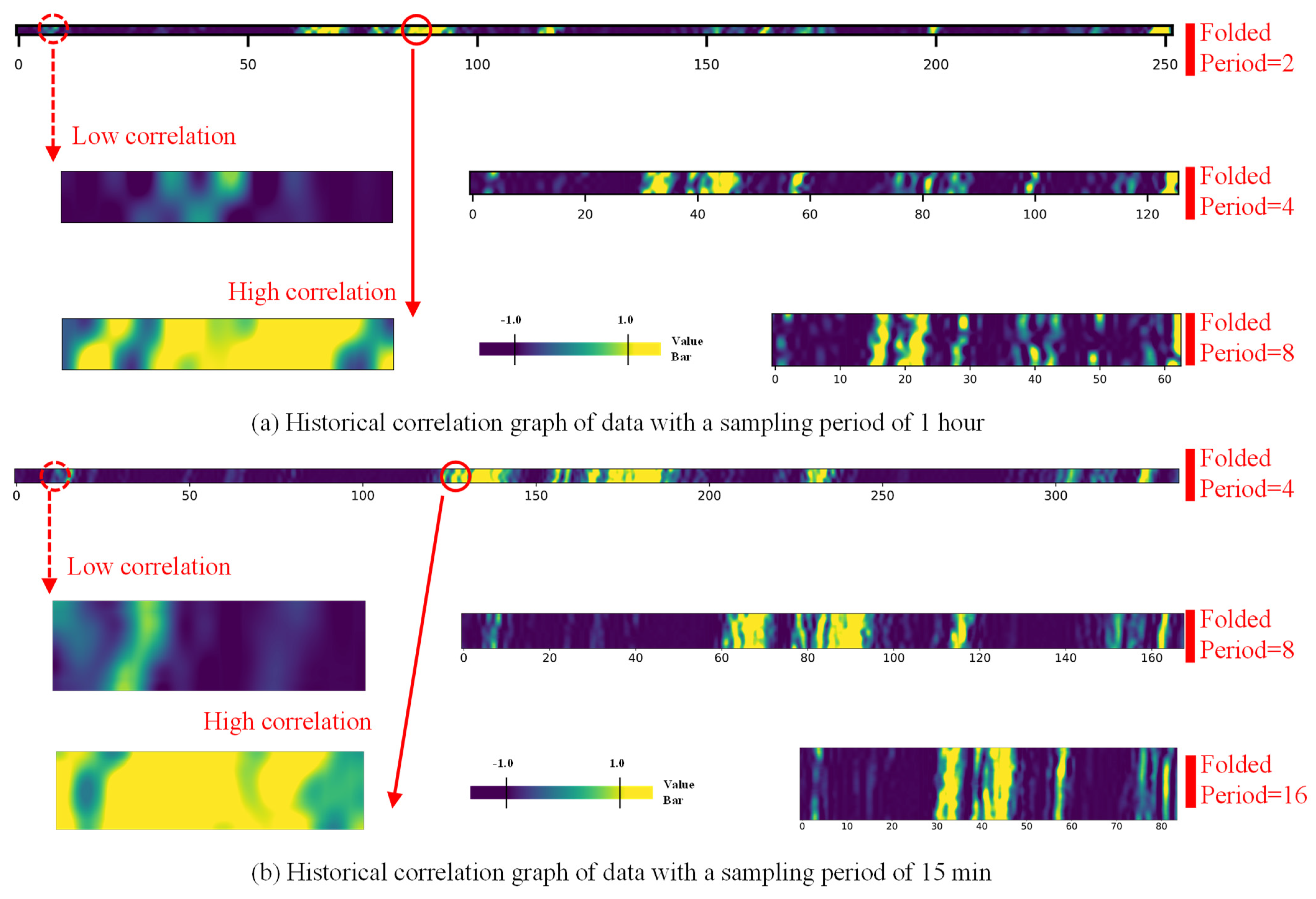
With the sampling frequencies of 15 min and 1 h, sampling time was 2 weeks, and the results are shown in Figure 2. If the historical data correlation graph were displayed point by point, the image would be too long and would not have a good observation effect. The folding period is in {2, 4, 8, 16} data points, and the folded data input is x L x ^ L / N × N . L is the length of the input sequence. N is the folding period. This correlation graph is more readable.
In the image with a 15 min sampling period and a folding period of 2, it can be seen that the historical correlation in wind power data changes over time. The darker the color, the lower value, which indicates a lower correlation. Conversely, as color brightness increases, the associated values increase, signifying a higher level of historical relevance. Within the entire length range, only 4–5 time windows show high correlation. The degree of correlation is low in most other time windows. High correlation data have lower dimensions and longer lengths. As the folding period increases, the data dimension increases and the length decreases. Different folding methods can lead to data presenting different features in a spatiotemporal range, which is also an important factor affecting prediction models.
In summary, regardless of the sampling period and folding dimension used for observation, the overall historical correlation in wind power data is relatively low. Only within a random and brief time window, a high correlation can be observed. Such data characteristics are not sufficient to support traditional deep learning models in learning historical representations, and can also bring uncertainty in prediction. While it may exhibit some efficacy in short-term forecasting, its performance diminishes significantly when applied to medium- to long-term forecasting. Specific experimental results can be found in Section 5.2.2. Therefore, it is necessary to study power prediction models that are suitable for both short-term and medium- to long-term power prediction based on such data characteristics.

2.3. Correlation Analysis of NWP Data

Due to the high fluctuation and the insufficiency of wind power data, it is inadequate to meet the demand of accurate power prediction only by mining its inherent data characteristics [28,29,30]. Utilizing NWP data, which are readily accessible and highly reliable, can aid in model extraction for comprehensive power feature analysis and extraction. In order to verify the validity of NWP data, the Pearson Correlation Coefficient (PCC) was used to calculate the correlation level between the data. Its calculation formula is as follows:
Corr = cov ( X , Y ) σ X σ Y = E [ ( X μ X ) ( Y μ Y ) ] σ X σ Y
where, X , Y show the power data and NWP data sequence; cov ( X , Y ) stands for the covariance between data; σ X , σ Y mean the variance in data; μ X , μ Y denote the average of data; and E denotes expectation.
In statistics, it is generally believed that, when Corr 0 . 6 , there is a strong correlation that exists between the data; when 0.4 < Corr < 0 . 6 , a moderate correlation is observed between the data; and, when Corr 0 . 4 , a weak correlation is evident between the data. In this paper, the annual power data and NWP data are analyzed by PCC, and a correlation score of Corr = 0 . 7044 is derived, which shows that there is a strong correlation between them.
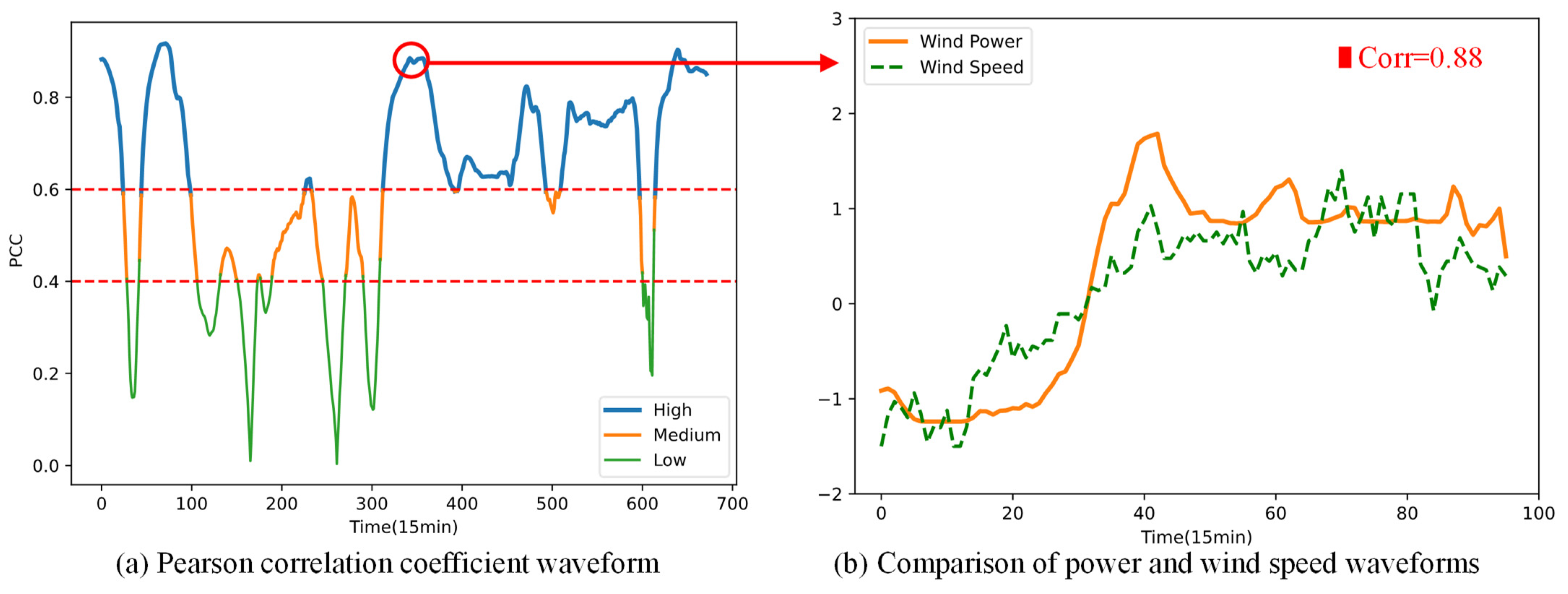
In addition, we took T = 96 as the sliding time window to select power data { P i , P i + 1 , , P i + T 1 } T × 1   and weather data { W i , W i + 1 , , W i + T 1 } T × F   , and calculated the correlation coefficients represented by wind speed and wind power output separately. We obtained the correlation waveform within 2 weeks, as shown in in Figure 3a.
As can be seen, for most of the time, the data exhibit a significant degree of correlation, with only brief periods of low correlation observed. To observe the correlation level of data more intuitively, the wind power data within one of the time windows were selected for waveform comparison as shown in Figure 3b. The correlation coefficient of this graph is 0.88. It can be seen that there is a high similarity between the trend in wind speed and the trend in power output over a 2-week time window. This also confirms that this set of data is highly correlated. Unlike the strong randomness in wind power, meteorological data such as wind speed can be accurately predicted through physical modeling and other methods, and the prediction technology is also relatively mature. Therefore, this section proves the high correlation between NWP data and wind power data, and verifies the feasibility of using it as auxiliary information to improve the accuracy of model prediction after feature fusion with historical data.

2.4. Data Preprocessing

To ensure the data quality and the efficiency of model calculation, it is necessary to process all data sources. This paper adopts three methods: data standardization, missing data filling, and abnormal data repair [31,32].

2.4.1. Z-Score Standardization

In this paper, both power data and NWP data are taken as the inputs of the model. Because the units of data are different, they are often on different orders of magnitude. To facilitate comparison and feature fusion, they must be unified on the same scale [33,34]. In addition, to facilitate the gradient calculation and back propagation of the depth model itself, the input data often need to be standardized. This paper adopts the Z-Score standardization method. Its advantages are that the algorithm is simple, it is not affected by the order of magnitude, and the results are easy to compare. The formula is below:
X new = X μ X σ X
where X stands for the raw data and X new represents the data after standardization. This method conducts standardized based on the mean and standard deviation of the original data. The processed data show normal distribution with a mean of 0 and a variance of 1.

2.4.2. Missing Data Filling

In the process of collecting NWP data, due to various reasons such as abnormal communication or equipment failure, data loss often occurs. A deep learning model normally cannot handle this kind of incomplete data input, so filling in missing data is necessary [18]. In order to ensure the quality of the filled data and avoid the interference of low-quality data on the model prediction, this paper adopts the K-Nearest Neighbor (KNN) filling algorithm [35]. The data points with missing values are filled with K adjacencies, and the distance matrix between the data points with missing values and other data points without missing values is calculated, and the K data points with the nearest Euclidean distance are selected. Filling the vacancy value in the data with the field average corresponding to the selected K-nearest neighbor data points, the data filling is finally achieved. The Euclidean distance formula is as follows:
d X , Y = i = 1 n ( X i Y i ) 2

2.4.3. Abnormal Data Repair

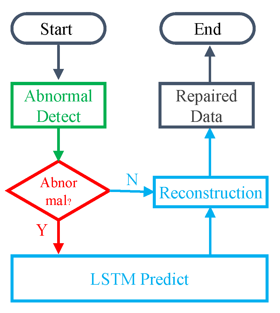
In the process of data sampling, in addition to losing data, abnormal data often appear. The characteristics of these data obviously deviate from the data in other locations, and may introduce significant interference to the prediction algorithm. Therefore, it is necessary to repair these abnormal data. Because these abnormal points generally occur with low frequency and short duration [36], after abnormal data are detected, the LSTM time series algorithm can be used to predict the location data of abnormal data according to historical data information, and the predicted value can replace the abnormal data to complete the data repair process [37,38,39]. The specific process is shown in Figure 4.

3. Introduction of Basic Principles

A Recurrent Neural Network (RNN) is a neural network that takes sequence data as input, recurses in the direction of sequence evolution, and all nodes (loop units) are connected in a chain. It has memory, parameter sharing, and Turing completeness. It has been commonly employed to address traditional time series prediction problems. This approach offers the advantage of being capable of handling input sequences of varying lengths and effectively retaining and recalling previous time information. As a result, it has found extensive application in ultra-short-term prediction scenarios. However, in the process of medium- and long-term prediction, its serial calculation mode suffers from the shortcomings of slow calculation speed, easy gradient explosion or disappearance, and information forgetting.
To address the limitation of RNN’s inability to process rows in parallel, this paper adopts the basic architecture of Transformer, and adds residual gating unit and hole convolution technology to process time series data in parallel. Its advantages are that the time sequence position information is preserved when processing time sequence data, and the data can be processed in parallel to speed up the operation. It is more competitive than RNN in prediction tasks and uses simple linear gating units to stack convolution layers, so that data can be processed in parallel while obtaining contextual semantic features. In addition, this paper also adopts the multi-head attention mechanism. An attention mechanism focuses on important information with high weight, ignoring irrelevant information with low weight. Moreover, the ability of dynamically adjusting its weights enables the selection of critical information in diverse contexts, enhancing its scalability and robustness.

3.1. Residual Gated Tanh Unit

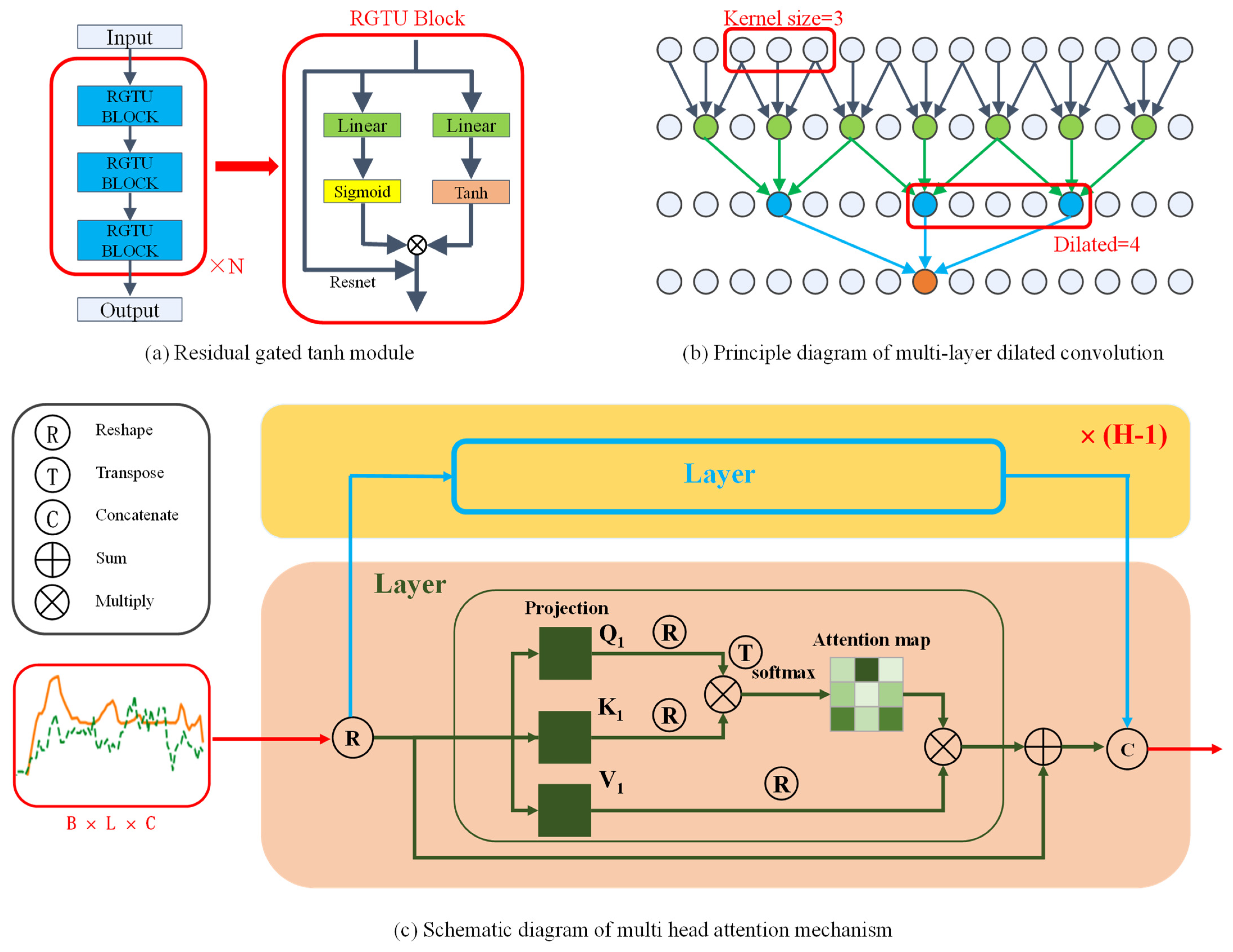
Residual gated tanh module is a gating unit based on residual logic. The specific structure is shown in Figure 5a. Each unit is composed of multiple blocks connected in series. The data are processed by stacking multiple units in series. The block is composed of two linear layers, a sigmoid layer, and a Tanh layer, with residual mechanisms added. Within the block, the data are mapped at different latitudes by two Linear layers, and then pass through Tanh layer and Sigmoid layer respectively. Among them, Sigmoid layer is one of the common Activation functions in neural networks, commonly used for hidden layer neuron output, with a value range of (0,1). It can map inputs to the interval of (0,1). This method is the core of the gating mechanism, which can realize Feature selection of multi-layer data. If the output of Sigmoid is closer to 1, the data information of that layer is retained more. If the output of Sigmoid is closer to 0, the changed data information is more discarded. In addition, to improve the efficiency of multi-layer model, residual structure is added to the element. The calculation formula of the gating unit is as follows:
h l ( X l ) = tanh ( X l W l + b l ) σ ( X l V l + c l )
where X l and h l ( X l ) is the l-th unit input and output, h l ( · ) is the function of the l-th unit, W l and V l are the weight of two linear layers, b l and c l are the offset of two linear layers, σ represents the Sigmoid algorithm, and tanh symbolizes the hyperbolic tangent function.

3.2. Dilated Convolution Model

To further extract the temporal–spatial correlation in sequence data, this paper uses the Conv1d convolution method to extract and fuse features of data with different dimensions.
In convolution, the Kernel is a weight array that weights the input data and is the core of computation. As the Kernel size increases, the model can capture larger features, but it increases the number of parameters and computational complexity, and may lead to overfitting. When the Kernel size is reduced, the model can capture more detailed features, but it may lose some important information. Therefore, selecting an appropriate Kernel size is crucial for the performance of the model.
In this paper, the dilated convolution method is used to extract features, and the specific structure is shown in Figure 5b. Differently from the traditional convolution method, the dilated convolution introduces hyperparameters of the differentiation rate. It increases the distance between the Kernel’s data processing, so as to achieve a higher Receptive field.
When Kernel size = 3 and dilated = 4, the same convolution Kernel can capture data information with a distance of 3 ∗ 4 = 12. That is to say, in the case of the same feature map, dilated convolution can obtain a larger receptive field and obtain more dense data on the premise of retaining data characteristics.

3.3. Multi-Head Attention Mechanism

Multi-attention mechanism is one of the main modules in Transformer model. Through the calculation of attention weight, the model can capture more important data features, thus improving the prediction accuracy. Multi-head means that the model can pay attention to different spatial information in different positions by mapping multiple subspaces, so as to capture more abundant feature information.
The specific structure is shown in Figure 5c. In the figure, the multi-head attention mechanism is composed of H-layer single-head attention layers in parallel. After being transformed, the input information is mapped to different attention layers in the H layer for attention matrix calculation, and, finally, concatenated for output, i.e., the processed data x B × L × C x ˜ B × L × H × E with H subspaces after Reshape. B is the data batchsize. L is the length of data. C is the channel dimension. H is the head of attention. E = C/H is the feature dimension of each head. In the single-head attention mechanism, such input data can be directly processed. However, in the multi-head attention mechanism, dimensions need to be reorganized. Adopting a multi-head attention mechanism can pay attention to different spatial information in different positions by mapping multiple subspaces, so as to capture more abundant feature information.
In each subspace, the Query, Key, and Value matrices are obtained by three-layer linear mapping of Q, K, and V, respectively. The Attention map is calculated by QK, and then it is multiplied by Value after passing through SoftMax, to be finally merged with the data in other subspaces for output. To improve the efficiency of the model, a residual mechanism is also added. The formula is as follows:
Attention ( Q , K , V ) = softmax ( Q K T L ) V

4. Gated Transformer Models

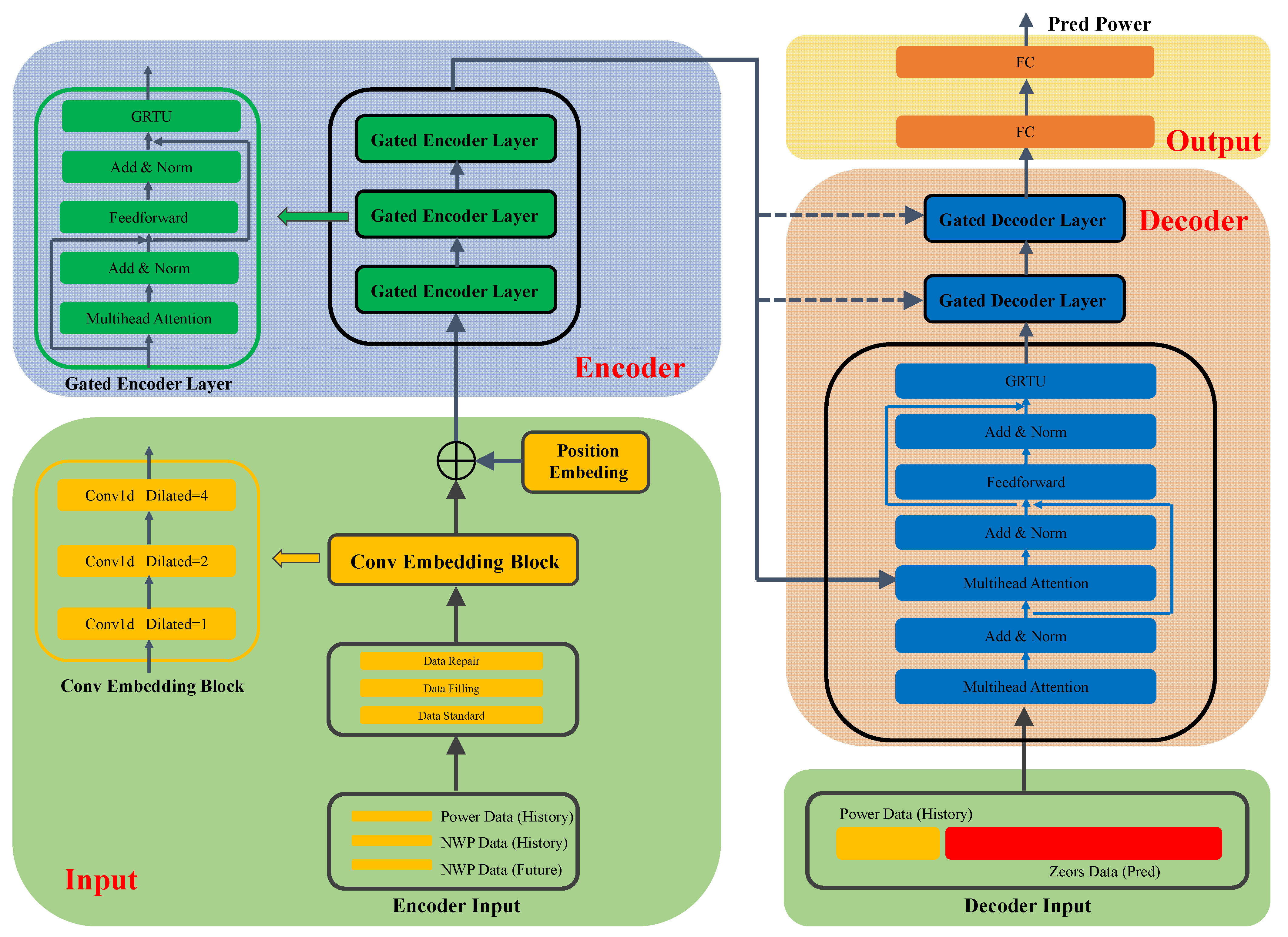
In order to effectively improve the accuracy of wind power prediction with strong fluctuation and randomness, this paper proposes a Transformer model based on a gating mechanism. The innovations of this model mainly include that NWP data information is introduced as auxiliary information, improving data correlation and ensuring the effectiveness of data feature extraction; that preprocessing techniques such as data standardization, data filling, and data repair are employed to enhance the quality of the data; that the hole convolution module is used to fuse and extract features of different dimensions; and that spatial position information is added to complete data reconstruction. Using a multi-head attention mechanism, overall information can be obtained from different subspace angles, and the expression ability is stronger. By applying the gated residual unit, the weight can be adjusted adaptively, the feature focus can be completed, and the operation efficiency can be improved. In Decoder input, a short piece of real historical data is preceded by 0 sequence to guide the direction of model prediction.
The whole model consists of four modules: Input module, Encoder module, Decoder module, and Output module. The data are encoded and processed through the Input module. After completing the feature fusion input to the Encoder module, it uses a self-attention mechanism to calculate the weight matrix of the sequence length and output it to the Decoder module. Considering the input information and weight matrix, the Decoder performs decoding operations. The output module maps vectors into prediction tasks, ultimately achieving power prediction. The model structure is shown in Figure 6 and the internal structure of each module is introduced in detail below.

4.1. Input Module

The Input module is mainly composed of Encoder Input and Decoder Input. Because the classic Transformer belongs to the Encoder–Decoder architecture, the input data types and formats on both sides are different. Therefore, while designing the inputs separately, it is also necessary to design two different network structures to meet the processing requirements for the inputs.

4.1.1. Encoder Input

  • Input data design:
The Input of Encoder mainly includes three data types. Historical wind power data are P = { P i , P i + 1 , , P i + T s 1 } B × T s × 1 , where P i is the i-th random data point as the starting point of historical input, P i + T s 1 is the endpoint of historical input, and the length of the historical power input sequence is T s . Historical NWP data are W = { W i , W i + 1 , , W i + T s 1 } B × T s × F . Similarly, this data sequence is a time series with a length of T s and a dimension of F. Future NWP data are collected by a meteorological prediction system and are W ˜ = { W i + T , W i + T + 1 , , W i + T + p 1 } B × T p × F . Unlike historical data, the length of the future sequence is T p , which depends on the length of the power which needs to be predicted;
  • Data processing design:
After data collection, data need to be preprocessed. Due to different types of data, the unit and fluctuation range of NWP data are inconsistent, so all the data are unified under the same scale by standardized method for observation. In addition, data filling and data repair are used to avoid the bad influence on the prediction model due to data loss or abnormality, and improve the data quality. During this process, the format of the input data does not change;
  • Dilated convolutional design:
Then, the data are fused and extracted by the dilated convolution module. To ensure the high efficiency of convolution calculation during the input of long sequence data, the module is designed to be composed of three pyramid-shaped cavity convolution layers. This scheme can expand the data receptive field and extract features more efficiently on the premise of maintaining the computational complexity. Here, the Conv1d convolution model is adopted and the dilated rates are set to be {1, 2, 4}. We introduce the padding mechanism to ensure consistency in length. In addition, dilated convolution is generally suitable for power prediction of long input sequences. In short-term prediction, too large of a Receptive field will lose the variability in the data themselves. Therefore, an adaptive approach is adopted, which can automatically adjust the dilated ratio during short-term input, thus ensuring the efficient feature extraction of convolution. Note that the format of the data will change B × T s × F B × T s × D , B × T p × F B × T p × D here, where D = 128 is the set hidden layer dimension;
  • Position embedding design:
Finally, the data reconstruction is completed through the position coding module. It encodes the given input sequence according to odd and even positions. The odd positions are encoded using cosine functions PE ( p o s , 2 i + 1 ) = cos ( p o s / 10000 2 i / D ) . Even positions are encoded according to sinusoidal positions PE ( p o s , 2 i ) = sin ( p o s / 10000 2 i / D ) . After completing the encoding, the location information is added to the data sequence.

4.1.2. Decoder Input

The input of the decoder is much simpler than that of the encoder. Since the Decoder module maintains the input and output dimensions unchanged and the future power data is unknown, the input is designed as { 0 , 0 , , 0 } B × T p × 1 which is an all-zero matrix with dimensions matching the predicted output. To further improve the accuracy of the model prediction, a short piece of guidance data composed of historical power data { P i + T s T L P i + T s 2 , P i + T s 1 } B × T L × 1 is added before the all-zero matrix to support prediction, where T L is the length of lead historical data.

4.2. Encoder Module

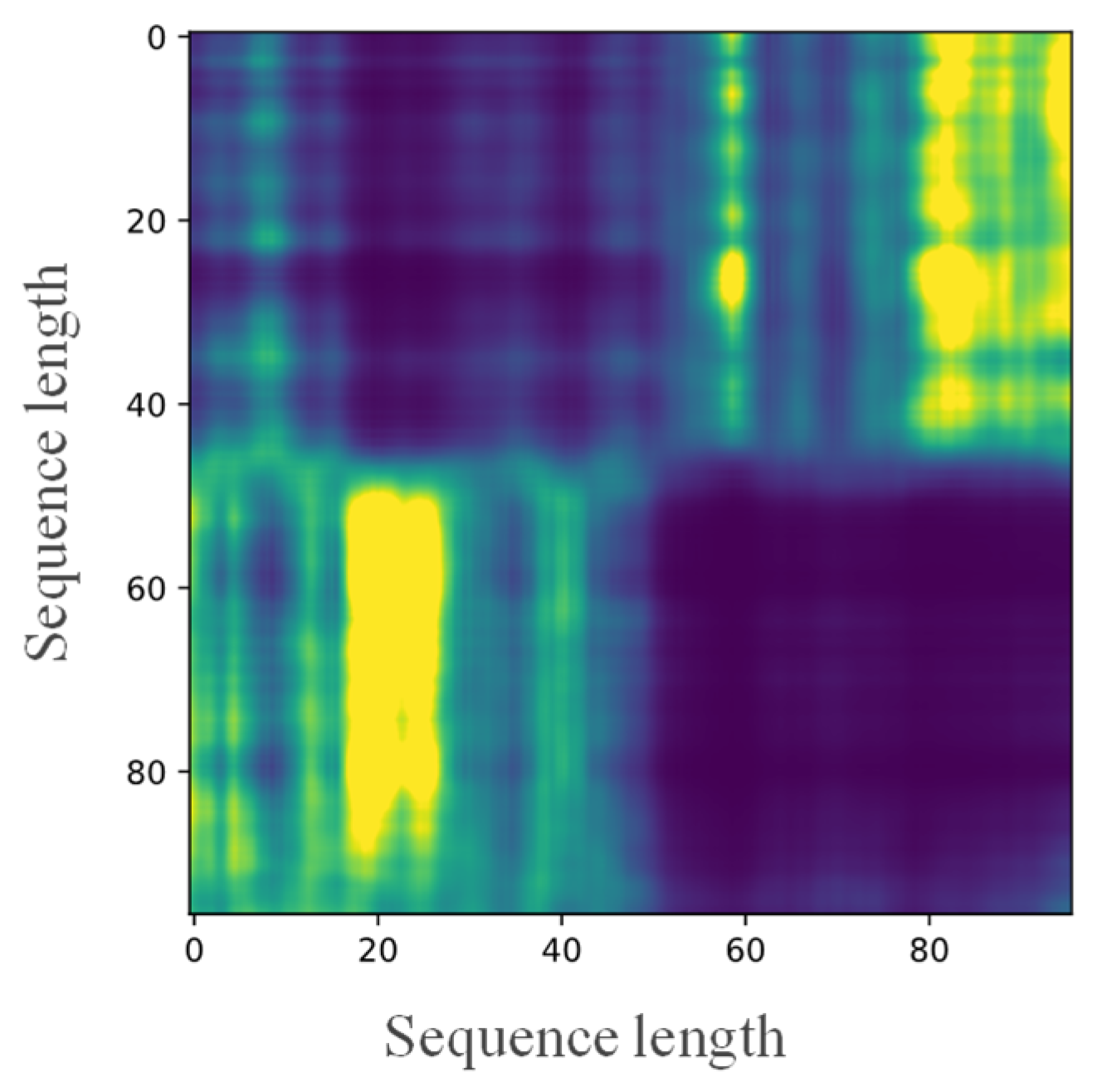
The Encoder module is mainly composed of multiple Encoder layers connected in series, and the number of layers can be set freely. In this paper, a three-layer structure is adopted. Each layer includes a multi-head attention mechanism, residual and regularization network, linear feedforward network, and GRTU module. The multi-head attention mechanism is set to 8 heads. The module can focus the input multi-dimensional feature information with attention weights, and output the attention diagram of B × T S × T S to Decoder, helping Decoder to complete the final power prediction.
In other words, the Encoder module is the core of the entire model. It can analyze and extract the features of input sequences, and utilize gating systems and attention mechanisms to efficiently capture the core intrinsic features of the data, thereby helping the Decoder to complete sequence prediction. As the Encoder outputs an attention weight map, it reflects the distribution of key information in the sequence. To facilitate understanding and observation, the output was visualized and shown in Figure 7. The figure shows the encoder output with an input length sequence of 96. It can be seen that the attention in the first and second half of the sequence is focused on itself, respectively. The poor attention at the front and back ends also reflects a low correlation.

4.3. Decoder Module

Like the Encoder module, the Decoder module is also composed of three Decoder Layers connected in series. Specifically, each Layer includes one self-attention, cross-attention, feed forward, residual and regularization network, and GRTU layer. It can be seen that, unlike the Encoder, the Decoder module has an extra layer of Cross-attention, which is utilized to input the attention information from the Encoder to Q and K. Then, it is multiplied by the mapping input V of Decoder to complete the data output. This module is the main structure to realize power prediction. Note that, since the output of the Decoder does not change the input dimension, it cannot be directly applied to power prediction. Therefore, it is necessary to add an output layer to map the feature space to the Sample space through linear changes.

4.4. Output Module

After the Decoder output, two FC layers are used to map the learned features into the sample space, and the final power prediction result is obtained.

5. Experiments

5.1. Experimental Configuration

This paper carries out data acquisition and simulation analysis on a computer with Tesla V100 GPU and 32 GB of VRAM which is created by NVIDIA in Santa Clara City in America. The program was implemented using the Python language within the PyTorch framework.
The proportions of training set, verification set, and test set were set to 70%, 15%, and 15%, respectively. The loss function used Mean Squared Error (MSE) and the optimizer used Adam optimizer. In the test set, evaluate Metrics were MSE and Mean Absolute Error (MAE).
The hyperparameter settings were as follows: Batchsize = 128; Learning rate = 1 × 10⁻⁴; Using kaiming weight initialization; Epoch = 400; Dropout = 0.1.
The steps of calculation are summarized in the pseudocode in Algorithm 1.
Algorithm 1: The pseudocode of calculation.
TRAIN
1Criterion is MSEloss.
2Optimizer is Adam.
3For X,y in TrainLoader:
4  Reconstruct Encoder and Decoder INPUT.
5  OUTPUT = model (INPUT)
6  Calculate loss.
7  Backpropagation and update parameter.
8End For
9Do VALID dataset and calculate test loss.
10Do TEST dataset and calculate valid loss.
VALID
1For X,y in ValidLoader:
2  Reconstruct Encoder and Decoder INPUT.
3  OUTPUT = model (INPUT)
4  Calculate loss.
5End for
6Return Valid Loss
TEST
1For X,y in TestLoader:
2  Reconstruct Encoder and Decoder INPUT.
3  OUTPUT = model (INPUT)
4  Calculate loss.
5End For
6Return TEST Loss

5.2. Comparison of Different Models’ Results

5.2.1. Models Introduction

To assess the effectiveness of the proposed approach, the Gated Transformer (G-Former) was compared against various classical power prediction methods, namely Deep Neural Networks (DNN), Gated Recurrent Unit network (GRU), Temporal Convolutional Network (TCN), Vanilla Transformer (V-Former), Encoder-only, Decoder-only, Informer, and Reformer. The following is a brief introduction to each model.
DNN: Deep Neural Network is based on linear layers structure. It consists of six blocks; each block layer consists of two linear layers. To ensure the efficiency of deep learning, a residual mechanism is added to each block. In addition, to further improve the recognition efficiency of linear layers, the Decomposition scheme used in Autoformer and FEDformer with linear layers is adopted. It first decomposes a raw data input into a trend component by a moving average kernel and a remainder (seasonal) component. Then, two one-layer linear layers are applied to each component, and sum up the two features to obtain the final prediction. By explicitly handling the trend, DNN enhances the performance of a vanilla linear when there is a clear trend in the data.
GRU: Gated Recurrent Unit network is a kind of Recurrent neural network, which can better capture the dependencies of time series data with large intervals. It consists of an update gate and a reset gate. The reset gate determines how to combine new input information with previous memory, while the update gate defines the amount of previous memory saved to the current time step. It can better solve the gradient problems in Long-term memory and back-propagation, so it is more suitable for medium–long-term power prediction.
TCN: Temporal Convolutional Network is a new algorithm that can be used to solve time series prediction, which has the ability to integrate modeling capabilities in the time domain and feature extraction capabilities in low parameter convolution. It is based on the convolutional model structure and uses causal convolution and residual mechanisms. It is characterized by parallel computing, flexible Receptive field, stable gradient, and variable input sequence.
VanillaTransformer: Vanilla Transformer is a deep learning model based on the Encoder–Decoder architecture. It can learn context and meaning by tracking relationships in sequence data, such as words in a sentence. This model applies a set of evolving mathematical techniques, called attention or self-attention, to detect even subtle ways in which remote data elements in a series interact with and depend on each other. In many cases, Transformer replaces traditional classical neural network models, which is currently the most popular type of deep learning model. It has high efficiency, has strong contextual awareness, and can be parallelized for computation.
Encoder-only: Encoder-only refers to retaining only the Encoder structure of the Transformer to complete the prediction task. It has a simple structure, faster training and inference speed, and advantages such as simple prediction, classification, annotation, and other tasks, while ensuring the same capabilities as the Transformer.
Decoder-only: Decoder-only refers to retaining only the Decoder structure of the Transformer to complete the prediction task. Its structure is simple and avoids some difficulties in Encoder–Decoder training, such as initialization of different weights and Information bottleneck method. In the training of the Decoder-only model, the output generated in the previous step is used as the input for the next step, which achieves self-supervision of the Decoder part and is conducive to generating more coherent and structured output sequences.
Informer: Informer is a Transformer based predictive model structure. It has a strong ability to align long time sequences and the ability to handle the input and output of long time sequences. Additionally, it solves the problem of traditional models being too thorough, or consuming GPU resources and server storage resources. While ensuring prediction accuracy, it reduces the computational complexity and memory usage of self-attention.
Reformer: Reformer is also a prediction model structure based on Transformer. It uses Axial Positional Embedding to reduce the position encoding matrix and proposes a segmented approach to handle the calculation process of the fully connected layer, calculating only a portion at a time, eliminating the need to load the entire sequence into memory, and using reversible residual connections instead of traditional residual connections. This is a solution for storing extreme compression.
The DNN model is composed of linear layers and lacks Feature selection, which also leads to the poor effectiveness of the model for complex tasks. GRU is specifically designed to handle time series problems and performs well in short-term prediction tasks. However, there are issues such as gradient vanishing in medium–long-term prediction tasks. TCN can complete feature extraction with a large Receptive field, but the lack of attention mechanism makes it difficult to select its Receptive field. Vanilla Transformer, as the basic framework of the most classic transformer model, has been widely used in multiple fields. However, it was originally designed to solve NLP problems and lacked optimization for time series. Encoder-Only and Decoder-Only models are optimized on the Transformer framework, with the advantage of halving the number of model parameters and retaining the advantages of the Transformer. The disadvantage is that these models have many layers, and the data efficiency is low because no Feature selection unit is added. The Informer and Reformer models adopt different compression schemes to ensure computational efficiency while ensuring the accuracy of time series prediction. However, this did not bring much accuracy improvement. Especially for the time series with poor autocorrelation such as wind power, the lack of data feature fusion and efficient Feature selection leads to the loss of prediction accuracy. Therefore, in order to solve the above problems, this paper proposes a model based on a gated transformer network.

5.2.2. Results Comparison

In order to ensure the scientific comparison of the experiments, five sets of experiments were conducted and the accuracy was judged based on the mean. The NWP Information design contrast experiment was added or not added from the short-term and medium–longterm power prediction tasks. The evaluation metrics consisted of MSE and MAE. The results obtained are shown in Table 1.
  • It can be seen that the introduction of NWP auxiliary information significantly improves the accuracy of power prediction. For short-term prediction tasks, the average prediction accuracy of introducing the NWP model is MSE = 0.0651. The average prediction accuracy of the model without introducing NWP data is MSE = 0.0678, meaning it improved prediction accuracy by 5%. For long-term prediction tasks, the average prediction accuracy of introducing the NWP model is MSE = 0.5470. The average prediction accuracy of the model without introducing NWP data is MSE = 1.1896. The prediction accuracy was improved by 117%. Therefore, introduction of NWP data can not only improve the accuracy of short-term predictions, but also significantly improve prediction accuracy in medium- to long-term tasks.
  • In addition, when comparing the prediction accuracy of different models, the proposed G-Former model has the best prediction performance in both short-term and medium- to long-term prediction tasks. For short-term tasks, the accuracy was improved by about 8%. For medium to long-term tasks, the accuracy was improved by about 11%. This also proves the superiority of the proposed scheme.

5.2.3. Results Visualization

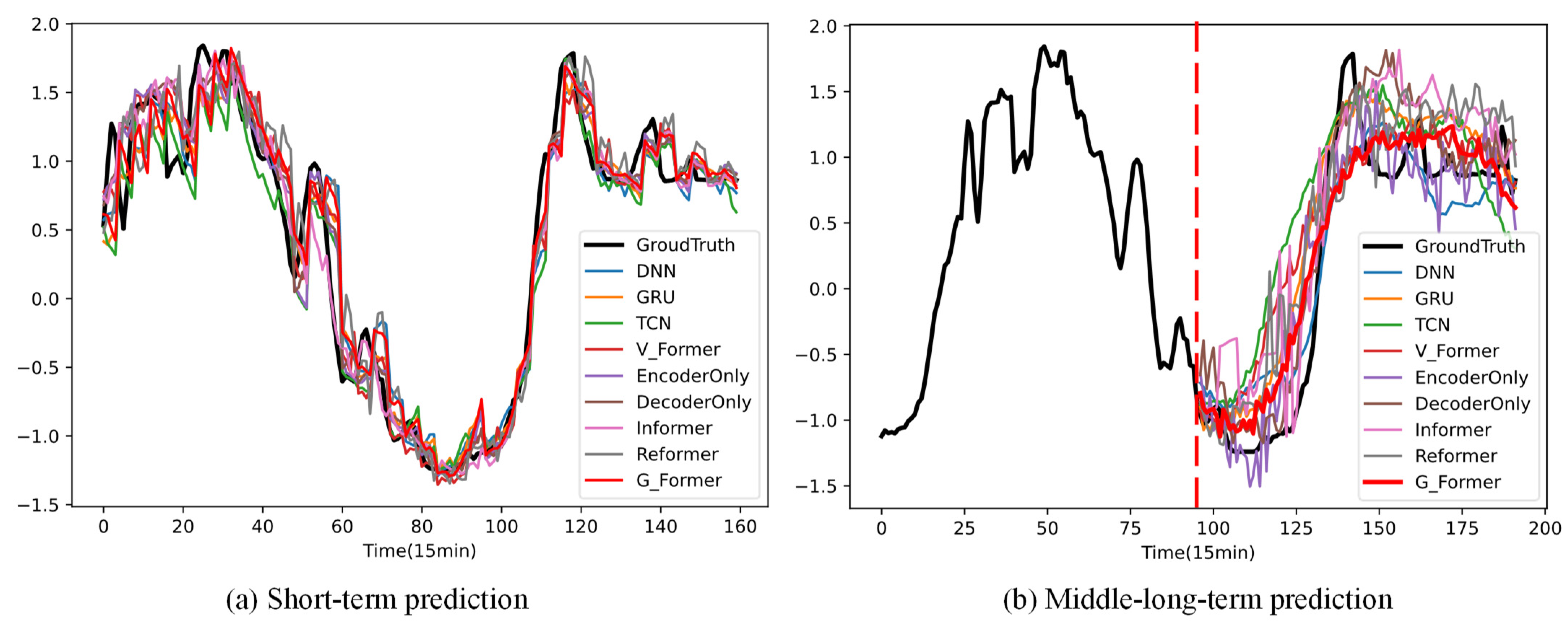
To facilitate the observation of the prediction accuracy of different models under different tasks, a visualization diagram of Comparison of predicted wave forms of different models is drawn in Figure 8.
Due to the fact that short-term predictions only predict waveform trends within the next few hours, the prediction time window is short and inconvenient to observe. Here, the rolling prediction method was used to predict the wind power data over two weeks, and the image is shown in Figure 8a. It can be observed that the proposed G-Former model is closest to the waveform of GroundTruth.
In medium–long-term prediction, experiments take the input sequence length of 96 and the predicted sequence length of 96 as an example to visualize and obtain the image, as shown in Figure 8b. It can be seen that, in the medium- to long-term prediction process, G-Former has the best prediction waveform.

5.3. Comparative Experiments on Different Time Scales

In order to further verify the predictive performance of the proposed model at different time scales, further experiments were conducted in this paper. The input sequence length and prediction sequence length were set to { 4 , 12 , 24 , 48 , 96 , 192 , 384 } . The prediction accuracy results are shown in Table 2.
It can be seen from the table that the length of the input and prediction sequences directly affects the accuracy of the prediction model, both when the input sequence is too short and the prediction sequence is too long. The model is unable to extract sufficient feature information from short sequences and is, thus, unable to achieve long-distance power prediction. When the input sequence is too long and the prediction sequence is relatively short, the data features of the input model are not concise enough, with a large amount of useless and redundant information, which can interfere with the model’s judgment. The model’s prediction performance is best when the lengths of the input and output sequences are within a reasonable range. Among them, for short-term prediction, a 24-step input sequence is sufficient to complete the model prediction. For medium- to long-term prediction models, if the length of the input sequence is generally consistent with the length of the predicted length sequence, the effect is best.
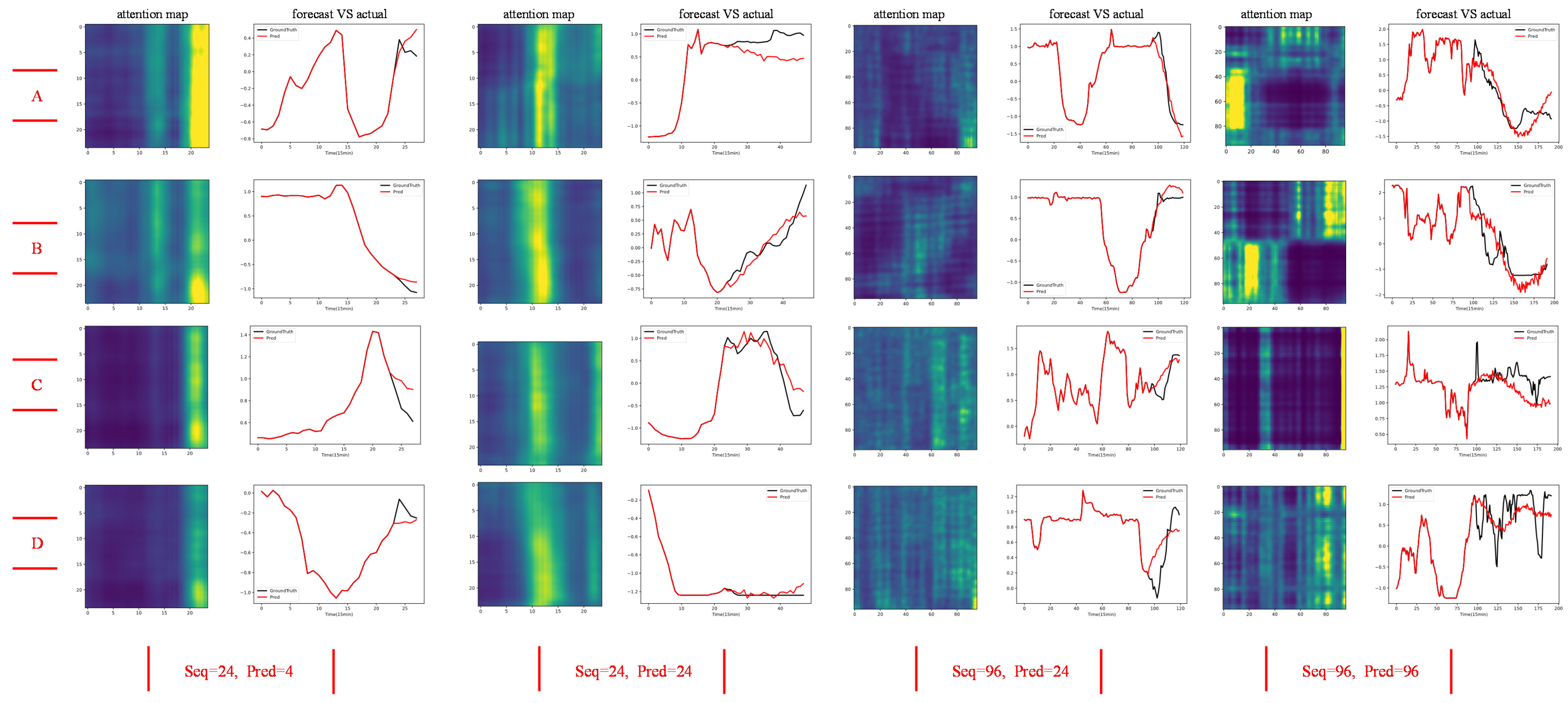
In order to further observe the predictive effect of the proposed model on different input and output sequence lengths, and achieve visualization of the output, this paper conducted experiments on typical prediction tasks { L s e q = 24 , L p r e d = 4 } , { L s e q = 24 , L p r e d = 24 } { L s e q = 96 , L p r e d = 24 } , { L s e q = 96 , L p r e d = 96 } . Furthermore, it randomly selected four sets of experimental data { A , B , C , D } to output prediction waveforms and Encoder attention maps. Each group of experimental results consists of an attention map of the input sequence and a comparison map of actual power and predicted power. The results are shown in Figure 9. It can be observed that the proposed scheme has good prediction performance at different time scales.

6. Conclusions

In this paper, a wind power prediction model based on a Gated Transformer is proposed. Firstly, the characteristics of wind power data are analyzed, and NWP information is introduced as auxiliary information to support prediction. Then, through data preprocessing, the data quality is improved. Secondly, the classical Transformer model is optimized by using a gating unit optimization, dilated convolution feature fusion, multi-head attention focusing, and Decoder input guidance. Finally, the effectiveness and reliability of the scheme are verified by a large number of comparative experiments. The main contributions of this paper can be summarized as follows:
(1)
The correlation between wind power data and NWP data is analyzed, which qualitatively explains the deficiency of feature extraction methods which only use historical data and demonstrates the necessity of introducing NWP data. Through data preprocessing, the data quality is improved;
(2)
Optimization of the classic Transformer structure is performed. The gating residual element is added to improve the feature focusing level between modules in series. By adding the dilated convolution module, multi-dimensional feature fusion is realized in a larger receptive field. The Encoder and Decoder input modules are redesigned, and historical data are used as guiding data to improve the prediction accuracy of the model;
(3)
The actual wind farm data are taken as an example to carry out simulation verification. By comparing the proposed scheme with the classical deep learning models, the superiority of the proposed scheme in MAE and MSE evaluation criteria is testified. After introducing NWP data information, the average accuracy of all prediction models in medium- to long-term prediction tasks can be improved by 117%. This verifies the necessity of introducing auxiliary information. For the same data source, GatedTransformer still shows an accuracy improvement of about 11%. This also verifies the superiority of the proposed method. In addition, the accuracy of prediction is also proven when the model uses input and output over different time scales.
This paper has made certain progress in the accuracy of medium–long-term prediction of wind power. However, this method has high requirements for the data quality of NWP. In addition, due to limitations in data sources, high-quality and supervised wind power datasets are not abundant enough, posing challenges to model training. The next work will mainly focus on combining the self-supervised model with the Gated Transformer to improve the training quality of the model through Pre-task.

Author Contributions

Conceptualization, Q.H. and Y.W.; methodology, Q.H. and Y.W.; software, S.-K.I.; validation, Q.H.; formal analysis, S.-K.I.; investigation, S.-K.I. and X.Y.; resources, Y.W.; data curation, Q.H.; writing—original draft preparation, Q.H.; writing—review and editing, Q.H. and Y.W.; visualization, Q.H. and Y.W.; supervision, Y.W.; project administration, Y.W. and X.Y.; funding acquisition, Y.W. and S.-K.I. All authors have read and agreed to the published version of the manuscript.

Funding

This research received no external funding.

Institutional Review Board Statement

Not applicable.

Informed Consent Statement

Not applicable.

Data Availability Statement

Not applicable.

Conflicts of Interest

The authors declare no conflict of interest.

References

  1. Vargas, S.; Telles, E.; Macaira, P. Wind Power Generation: A Review and a Research Agenda. J. Clean. Prod. 2019, 218, 850–870. [Google Scholar] [CrossRef]
  2. Aisyah, S.; Simaremare, A.; Adytia, D.; Aditya, I.A.; Alamsyah, A. Exploratory Weather Data Analysis for Electricity Load. Forecasting Using SVM and GRNN, Case Study in Bali, Indonesia. Energies 2022, 15, 3566. [Google Scholar] [CrossRef]
  3. Hong, Y.; Zhou, Y.; Li, Q.; Xu, W.; Zheng, X. A Deep Learning Method for Short-Term Residential Load Forecasting in Smart Grid. IEEE Access 2020, 8, 55785–55797. [Google Scholar] [CrossRef]
  4. Gong, M.; Zhao, Y.; Sun, J.; Han, C.; Sun, G.; Yan, B. Load forecasting of district heating system based on Informer. Energy 2022, 253, 124179. [Google Scholar] [CrossRef]
  5. Xie, W.; Zhang, P.; Chen, R. A Nonparametric Bayesian Framework for Short-Term Wind Power Probabilistic Forecast. IEEE Trans. Power Syst. A Publ. Power Eng. Soc. 2019, 34, 371–379. [Google Scholar] [CrossRef]
  6. Oh, E.; Wang, H. Reinforcement-Learning-based Energy Storage System Operation Strategies to Manage Wind Power Forecast Uncertainty. IEEE Access 2020, 08, 20965–20976. [Google Scholar] [CrossRef]
  7. Arani, M.; Mohamed, A. Dynamic Droop Control forWind Turbines Participating in Primary Frequency Regulation in Microgrids. IEEE Trans. Smart Grid 2018, 9, 5742–5751. [Google Scholar] [CrossRef]
  8. You, G.; Hang, Z.; Chen, K.; Liu, C.; Qian, Y.; Li, C. Wind turbine generator frequency control based on improved particle swarm optimization. Electr. Power Eng. Technol. 2020, 39, 43–50. [Google Scholar]
  9. Hu, T.; Zhang, X.; Cao, X. A hybrid particle swarm optimization with dynamic adjustment of inertial weight. Electron. Opt. Control 2020, 27, 16–21. [Google Scholar]
  10. Huang, C.; Kuo, C.; Huang, Y. Short-term wind power forecasting and uncertainty analysis using a hybrid intelligent method. IET Renew. Power Gener. 2017, 11, 678–687. [Google Scholar] [CrossRef]
  11. Shahid, F.; Khan, A.; Zameer, A. Wind power prediction using a three stage genetic ensemble and auxiliary predictor. Appl. Soft Comput. 2020, 90, 106151. [Google Scholar] [CrossRef]
  12. Zhou, T.; Wang, Y.; Quan, H.; Zhang, T. Stepwise Inertial Intelligent Control for Wind Power Frequency Support Based on Modified Stacked Denoising Autoencoder. Energy Rep. 2022, 8, 946–957. [Google Scholar] [CrossRef]
  13. Lai, J.; Wang, X.; Xiang, Q.; Song, F. Review on autoencoder and its application. J. Commun. 2021, 42, 218–230. [Google Scholar]
  14. Song, L.; Fan, Y.; Liu, M.; Bai, X.; Zhang, X. State estimation method of a new energy power system based on SC-DNN and multi-source data fusion. Power Syst. Prot. Control. 2023, 51, 177–187. [Google Scholar]
  15. Jiang, H.; Liu, Y.; Feng, Y.; Zhou, B.; Li, Y. Analysis of power generation technology trend in 14th five-year plan under the background of carbon peak and carbon neutrality. Power Gener. Technol. 2022, 43, 54–64. [Google Scholar]
  16. Ouyang, T.; Zha, X.; Qin, L. Wind power ramp events forecast method based on similarity correction. Proceeding CSEE 2017, 37, 572–580. [Google Scholar]
  17. Liu, S.; Zhu, Y.; Zhang, K. Short- term wind power forecasting based on error correction ARMAGARCH model. Acta Energ. Sol. Sin. 2020, 41, 268–275. [Google Scholar]
  18. Han, L.; Zhang, R.; Wang, X. Multi- step wind power forecast based on VMD-LSTM. IET Renew. Power Gener. 2019, 13, 1690–1700. [Google Scholar] [CrossRef]
  19. Wang, X.; Cai, X.; Li, Z. Ultra- short- term wind power forecasting method based on a cross LOF preprocessing algorithm and an attention mechanism. Power Syst. Prot. Control. 2020, 48, 92–99. [Google Scholar]
  20. Andrade, J.; Bessa, R. Improving renewable energy forecasting with a grid of numerical weather predictions. IEEE Trans. Sustain. Energy 2017, 8, 1571–1580. [Google Scholar] [CrossRef] [Green Version]
  21. Yang, M.; Bai, Y. Ultra- short- term prediction of wind power based on multi-location numerical weather prediction and gated recurrent unit. Autom. Electr. Power Syst. 2021, 45, 177–183. [Google Scholar]
  22. Hu, S.; Xiang, Y.; Shen, X. Wind power prediction model considering meteorological factor and spatial correlation of wind speed. Autom. Electr. Power Syst. 2021, 45, 28–36. [Google Scholar]
  23. Jiaqi, S.; Jianhua, Z. Load Forecasting Based on Multi-model by Stacking Ensemble Learning. Proc. CSEE 2019, 39, 4032–4042. [Google Scholar]
  24. Ak, R.; Li, Y.F.; Vitelli, V.; Zio, E. Adequacy assessment of a wind-integrated system using neural network-based interval predictions of wind power generation and load. Int. J. Eelec. Power 2018, 95, 213–226. [Google Scholar] [CrossRef] [Green Version]
  25. Yuan, X.H.; Chen, C.; Yuan, Y.B.; Huang, Y.H.; Tan, Q.X. Short-term wind power prediction based on LSSVMGSA model. Energy Convers. Manag. 2015, 101, 393–401. [Google Scholar] [CrossRef]
  26. Wang, K.; Qi, X.; Liu, H.; Song, J. Deep belief network based k-means cluster approach for short-term wind power forecasting. Energy 2018, 165, 840–852. [Google Scholar] [CrossRef]
  27. Zang, H.; Liang, Z.; Guo, M.; Qian, Z.; Wei, Z.; Sun, G. Short-term wind speed forecasting based on an EEMD-CAPSO-RVM model. In Proceedings of the 2016 IEEE PES Asia-Pacific Power and Energy Engineering Conference (APPEEC), Xi’an, China, 25–28 October 2016; pp. 439–443. [Google Scholar]
  28. Mi, X.; Liu, H.; Li, Y. Wind speed forecasting method using wavelet, extreme learning machine and outlier correction algorithm. Energy Convers. Manag. 2017, 151, 709–722. [Google Scholar] [CrossRef]
  29. Jie, Y.; Chengzhi, X.; Yongqian, L. Short-term Wind Power Prediction Method Based on Wind Speed Cloud Model in Similar Day. Autom. Electr. Power Syst. 2018, 42, 53–59. [Google Scholar]
  30. Abedinia, O.; Bagheri, M.; Naderi, M.; Ghadimi, N. A new combinatory approach for wind power forecasting. IEEE Syst. J. 2020, 14, 4614–4625. [Google Scholar] [CrossRef]
  31. Liu, Y.; Guan, L.; Hou, C.; Han, H.; Liu, Z.; Sun, Y.; Zheng, M. Wind power short-term prediction based on LSTM and discrete wavelet transform. Appl. Sci. 2019, 9, 1108. [Google Scholar] [CrossRef] [Green Version]
  32. Wang, S.; Li, M. Short-term wind power prediction based on improved small-world eural network. Neural Comput. Appl. 2019, 31, 3173–3185. [Google Scholar] [CrossRef]
  33. Zhang, X.; Chen, Y.; Yue, S.; Zha, X.; Zhang, D.; Xue, L. Retrospect and prospect of research on frequency regulation technology of power system by wind power. Power Syst. Technol. 2018, 42, 1793–1803. [Google Scholar]
  34. Vyver, J.V.; Kooning, J.D.; Meersman, B.; Vandevelde, L.; Vandoorn, T.L. Droop Control as an Alternative Inertial Response Strategy for the Synthetic Inertia onWind Turbines. IEEE Trans. Power Syst. 2016, 31, 1129–1138. [Google Scholar] [CrossRef]
  35. Lu, Z.; Tang, H.; Qiao, Y.; Tian, X.; Chi, Y. The impact of power electronics interfaces on power system frequency control: A review. Electr. Power 2018, 51, 51–58. [Google Scholar]
  36. Wen, Y.; Yang, W.; Lin, X. Review and prospect of frequency stability analysis and control of low-inertia power systems. Electr. Power Autom. Equip. 2020, 40, 211–222. [Google Scholar]
  37. Klampanos, I.; Davvetas, A.; Andronopoulos, S.; Pappas, C.; Ikonomopoulos, A.; Karkaletsis, V. Autoencoder-driven weather clustering for source estimation during nuclear events. Environ. Model. Softw. 2018, 102, 84–93. [Google Scholar] [CrossRef] [Green Version]
  38. Zhang, J.; Yan, J.; Infield, D.; Liu, Y.; Lien, F.-S. Short-term forecasting and uncertainty analysis of wind turbine power based on long short-term memory network and gaussian mixture model. Appl. Energy 2019, 241, 229–244. [Google Scholar] [CrossRef] [Green Version]
  39. Wang, J.; Niu, T.; Lu, H.; Yang, W.; Du, P. A Novel Framework of Reservoir Computing for Deterministic and Probabilistic Wind Power Forecasting. IEEE Trans. Sustain. Energy 2019, 11, 337–349. [Google Scholar] [CrossRef]
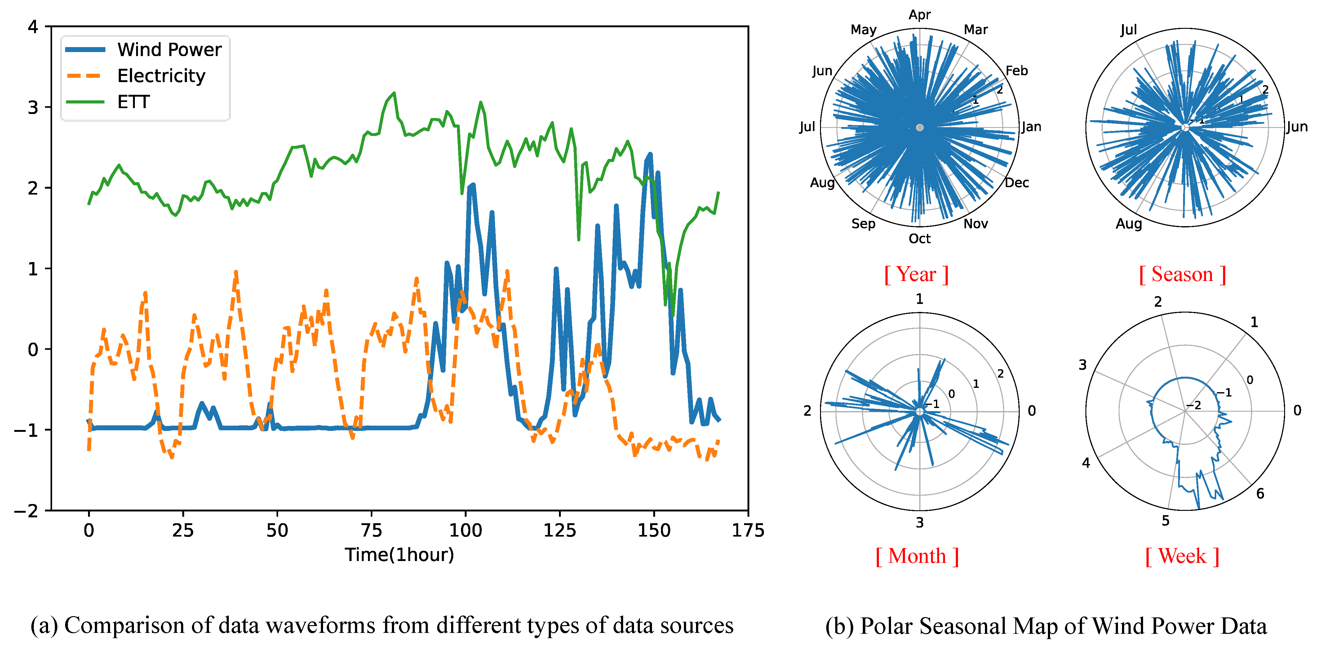
Figure 1. The chart of wind power characteristic analysis. All data are standardized by Z-Score. The sampling period is 1 h.
Applsci 13 08350 g001
Figure 2. The chart of historical data correlation analysis. The higher the historical correlation, the brighter the image. In the opposite case, it becomes darker.
Applsci 13 08350 g002
Figure 3. The chart of NWP data correlation analysis. All data are standardized by Z-Score. The sampling period is 15 min.
Applsci 13 08350 g003
Figure 4. The flowchart of data repairment.
Applsci 13 08350 g004
Figure 5. Chart of the basic unit model structure.
Applsci 13 08350 g005
Figure 6. The pipeline of the gated transformer.
Applsci 13 08350 g006
Figure 7. Encoder output attention map. The brighter the image, the more focused the attention.
Applsci 13 08350 g007
Figure 8. Comparison of predicted waveforms of different models. All data are standardized by Z-Score. The sampling period is 15 min.
Applsci 13 08350 g008
Figure 9. Comparison of predicted waveforms of different models. All data are standardized by Z-Score. The sampling period is 15 min. Each group of experimental results consists of an attention map of the input sequence and a comparison map of actual power and predicted power. (AD) is the randomly selected four sets of experimental data.
Applsci 13 08350 g009
Table 1. Comparison table of predictive performance of different models. The smaller the value, the better the performance. The best results are highlighted in bold and underlined.
ModelWith NWPWithout NWP
LengthShort TermMedium–Long-TermShort TermMedium–Long-Term
MetricMSEMAEMSEMAEMSEMAEMSEMAE
DNN 0.0721 0.0012 + 0.0008 0.1641 0.0025 + 0.0061 0.6491 0.0280 + 0.0116 0.5498 0.0165 + 0.0063 0.0747 0.0020 + 0.0019 0.1701 0.0054 + 0.0080 1.1728 0.0068 + 0.0037 0.9143 0.0032 + 0.0023
GRU 0.0599 0.0021 + 0.0015 0.1436 0.0028 + 0.0025 0.5626 0.0300 + 0.0142 0.5083 0.0121 + 0.0048 0.0641 0.0007 + 0.0010 0.1482 0.0268 + 0.0059 1.2014 0.0268 + 0.0112 0.9182 0.0055 + 0.0052
TCN 0.0636 0.0018 + 0.0023 0.1432 0.0027 + 0.0035 0.5308 0.0121 + 0.0409 0.5661 0.0083 + 0.0250 0.0645 0.0010 + 0.0009 0.1495 0.0057 + 0.0043 1.1538 0.0123 + 0.0099 0.9031 0.0062 + 0.0048
V-Former 0.0675 0.0054 + 0.0105 0.1651 0.0084 + 0.0116 0.5756 0.0202 + 0.0134 0.5316 0.0085 + 0.0071 0.0761 0.0050 + 0.0060 0.1672 0.0048 + 0.0048 1.2603 0.0179 + 0.0215 0.9248 0.0226 + 0.0319
Encoder-only 0.0615 0.0024 + 0.0022 0.1471 0.0079 + 0.0060 0.5315 0.0547 + 0.0368 0.5419 0.0291 + 0.0275 0.0650 0.0010 + 0.0010 0.1458 0.0058 + 0.0038 1.1785 0.0205 + 0.0212 0.9003 0.0060 + 0.0079
Decoder-only 0.0654 0.0042 + 0.0042 0.1515 0.0096 + 0.0047 0.5324 0.0258 + 0.0211 0.5183 0.0240 + 0.0080 0.0651 0.0024 + 0.0020 0.1462 0.0078 + 0.0044 1.1910 0.0255 + 0.0196 0.9045 0.0142 + 0.0152
Informer 0.0672 0.0034 + 0.0014 0.1559 0.0058 + 0.0046 0.5252 0.0242 + 0.0136 0.5005 0.0096 + 0.0311 0.0647 0.0106 + 0.0041 0.1562 0.0063 + 0.0081 1.1621 0.0167 + 0.0246 0.8922 0.0246 + 0.0310 ¯
Reformer 0.0729 0.0017 + 0.0022 0.1692 0.0061 + 0.0037 0.5297 0.0369 + 0.0401 0.5165 0.0306 + 0.0316 0.0725 0.0069 + 0.0011 0.1531 0.0265 + 0.0174 1.2336 0.0472 + 0.0654 0.9539 0.0553 + 0.0241
G-Former 0.0555 0.0014 + 0.0019 ¯ 0.1376 0.0023 + 0.0045 ¯ 0.4861 0.0050 + 0.0092 ¯ 0.4850 0.0062 + 0.0106 ¯ 0.0631 0.0005 + 0.0010 ¯ 0.1408 0.0022 + 0.0017 ¯ 1.1526 0.0102 + 0.0084 ¯ 0 . 9023 0.0150 + 0.0064
Table 2. Performance table of gated transformer at different time scales. The smaller the value, the better the performance. The best results are highlighted in bold and underlined. L seq is the length of the input sequence. L pred is the length of the pred sequence. “/” indicates the accuracy is too low and, therefore, meaningless in the specific situation.
L seq L pred
412244896192384
MSEMAEMSEMAEMSEMAEMSEMAEMSEMAEMSEMAEMSEMAE
40.06080.14600.31130.41090.64290.59870.87360.73301.23110.9496////
120.05730.14140.17880.25700.28830.37700.46640.46260.81060.70381.15040.8942//
240.05480.13830.17520.24660.29760.38820.41890.42360.67690.61751.09120.8466//
480.05990.14730.17880.25760.30700.34650.38110.41420.54560.52721.01700.7934//
960.06380.15350.19400.27560.31080.35560.47420.45740.48610.48500.81650.66691.34810.9780
1920.06140.15180.20350.28290.31750.36250.43820.44400.54430.50710.54870.54591.06970.8089
3840.07330.17720.20710.28980.33080.39530.47990.46700.47460.49060.59120.56890.67180.6055
Disclaimer/Publisher’s Note: The statements, opinions and data contained in all publications are solely those of the individual author(s) and contributor(s) and not of MDPI and/or the editor(s). MDPI and/or the editor(s) disclaim responsibility for any injury to people or property resulting from any ideas, methods, instructions or products referred to in the content.