Application of a Local Dynamic Model of Large Eddy Simulation to a Marine Propeller Wake

Abstract

With recent development of computer technology, the use of large eddy simulation method to solve industrial problems is gaining acceptance. From a theoretical and applied perspective, a local dynamic k-equation subgrid-scale model is applied to study the flow over a marine propeller. This local dynamic SGS model of LES have already been used in simple flows such as classical Taylor-Green vortex flow to investigate its robustness and superior than other dynamic SGS models. In this paper it will be applied to a more complex flows, i.e., simulation of a marine propeller wake, to further evaluate its ability range. 42 intentionally selected numerical experiments were conducted. The results of this local dynamic model of LES shows some superior than the dynamic Smagorinsky model, and well captures the wake evolution mechanism of a propeller, although which actually depends on its geometry.

1. Introduction

With today’s largest computers, it is not sustainable to apply direct numerical simulation (DNS) to numerically solve the complex flow such as flows around a propeller or a wind turbine. Realizing the limitations of classical statistical methods based on the Reynolds averaged Navier-Stokes (RANS) equations, a better solution may be large eddy simulation (LES). LES has lower computational cost than DNS and is more accurate than RANS simulation. Application of LES of rotor-like devices (such as propeller, wind turbine and helicopter) is challenging because of the complex geometry involved and the meshing strategy balancing accuracy and cost accepted. In this paper a local dynamic k-equation subgrid-scale (SGS) model is applied to study the flow over a David Taylor Model Basin marine propeller 4381 (DTMB p4381) from a theoretical and applied point of view.

In reference [1], a high fidelity large eddy simulation of a seven blade submarine propeller was carried out on a computational grid consisting of 840 million points, which combined with the acoustic model. The large eddy model uses the wall adaptive local eddy viscosity (WALE) model [2]. This kind of calculation cost is too high, and if there is no in-depth and rigorous discussion of the concrete LES model details, the results obtained are to some extent meaningless, or we can adopt a lower calculation cost model or strategy to achieve similar results. The literature [3] used 181 million unstructured grids composed of hexahedron elements only to conduct large eddy simulation for marine five blade propeller, and the use of dynamic Smagorinsky model was not described in detail. The billions of computing grids still hinder most researchers from practicing. We may obtain comparable conclusions through lower computational costs. Literature [4] used large eddy simulation to study the flow around a counter rotating propeller in uniform free streaming. The large eddy model used the dynamic Smagorinsky model proposed by Germano et al. [5] and modified by Lilly [6]. Using a computational grid with two levels of refinement, the fine grid has approximately 19.3 million grid units and the coarse grid has about 7.7 million. The results indicate that the consistency of the load and velocity fields around the propeller between the two grids and the experimental results are encouraging. Reference [7] uses large eddy simulation method to predict the flow around ship propeller in forward and backward operation modes, and the large eddy model also uses the dynamic Smagorinsky model. The minimum grid size is $1.7\times {10}^{-3}$ times the diameter of the propeller, with a total grid count of approximately 13 million. The simulated thrust and torque coefficients, circumferential average speed, and root mean square fluctuation of speed were compared with experimental data, and good consistency was observed.

Reference [8] used large eddy simulation to simulate the flow around a marine propeller and verified it with particle image velocimetry (PIV). The large eddy model uses dynamic large eddy simulation, delayed discrete eddy simulation (DDES) and stress mixed eddy simulation. The numerical results are compared with the experimental data to verify the effectiveness of the methods used. In recent years, more and more researchers have used PIV testing to measure and analyze the velocity information of propeller wake, as it can measure a large range of areas in a relatively short time. Reference [9] conducted experimental research on a small unmanned aerial vehicle propeller with serrated trailing edges, using a high-resolution digital PIV system to measure the flow field and quantify the detailed flow structure around the propeller. Reference [10] used PIV measurements of the wake flow field of a large oil tanker to validate two-dimensional PIV measurements and reconstruct three-dimensional flow fields by overlaying two-dimensional measurements, and studied the influence of rotating propellers on average velocity and turbulence characteristics. Reference [11] adopts a new type of underwater micro PIV system, which utilizes underwater particle image velocimetry and acoustic Doppler velocimetry to in-situ measure sediment resuspension caused by propeller erosion. Literature [12] carried out PIV analysis on the wake of rotating propeller in cavitation wind tunnel, and studied the wake characteristics of four propellers at high Reynolds number using dual frame PIV technology.

In this paper, from a theoretical and applied point of view, a local dynamic k-equation subgrid-scale (LES-LDKSGS) model is applied to study the flow over a marine propeller. This local dynamic SGS model of LES have already been used in simple flows such as classical Taylor-Green vortex flow, rearward facing step and so on to investigate its robustness. In this paper it will be applied to a more complex flows, i.e., simulation of a marine propeller wake, to further evaluate its ability range. Results from this SGS model of LES show promising trend to predict the complex dynamics of rotor flows effectively and accurately. The purpose of this study is to:

• Perform a LES simulation with a local dynamic k-equation eddy-viscosity model (named LES-LDKSGS in this paper) and a RANS simulation with a standard $k-\epsilon$ model (named RANS-kEpsilon, just for comparison with LES-LDKSGS) for flow over a submarine propeller at design and off-design advance ratios;
• Evaluate the ability of LES-LDKSGS model to capture the complex evolution of propeller wake, and compare the results of LES-LDKSGS model with the results of PIV measurements, dynamic algebraic model (LES-DASGS, also called LES-DSM) and RANS-kEpsilon model;
• Study the flow field evolution mechanics of the propeller and the origin of loads on blades from the perspective of engineering applications;
• Discuss vortex identification of the wake in detail from an academic point of view.

The organized structure of this article is as follows: firstly, numerical experiments are described in Section 2, including governing equations of the flow, LES models, propeller geometry, computation domain setting, initial conditions (ICs), boundary conditions (BCs), meshing strategy and numerical methods; then Section 3 provides validation of numerical simulations, including comparisons with physical experiments and other researcher’s LES-DSM simulation results; numerical experimental results are presented and discussed in Section 4; finally, based on the previous description and discussion, a summary is given in Section 5.

2. Numerical Experiments

2.1. Governing Equations of Flow

Fluid dynamics is controlled by three conservation laws of classical mechanics, namely, the conservation of mass, momentum and energy. Partial differential equations (PDEs) can be derived from these conservation laws and simplified in appropriate cases. These conservation laws are derived under the assumption of continuum mechanics, and we can then express the physical characteristics of flow (including velocity, pressure, density, etc.) as time-dependent scalars or vectors in three-dimensional space ${\mathcal{R}}^3$, such as pressure $p(t,\mathit{x})$ and velocity $\mathit{u}(t,\mathit{x})$. For liquids, such as the water used in this article, the continuity assumption always holds in practice.Flow can be represented in the Eulerian formulation as a time history of flow properties at each fixed point in a space domain. According to three laws of conservation, the continuity, momentum and energy equations in an arbitrary material volume $\mathit{V}\left(t\right)$ with surface $\mathit{S}\left(t\right)$ are derived [13], they (totally called general N-S equations) are as follows, herein Einstein summation convention (1916) is used.

$$\frac{\partial \rho }{dt}+{\left(\rho u_i\right)}_{,i}=0$$

(1)

$$\frac{\partial \left(\rho u_i\right)}{\partial t}+{\left(\rho u_i{u}_j\right)}_{,j}={\tau }_{ij,j}+\rho f_i^b$$

(2)

$$\frac{\partial \left(\rho E\right)}{\partial t}+{\left(\rho u_{i}E\right)}_{,i}={\left(u_i{\tau }_{ij}\right)}_{,j}+\rho u_i{f}_i^b+\rho q+{\left(k{T}_{,i}\right)}_{,i}$$

(3)

where, $\mathbf{\tau }$ is the stress tensor, ${\mathit{f}}^b$ is the body force per mass acting on a material particle, $E=e+0.5u_i{u}_i$ is the total energy per unit mass, e is the internal energy per mass, $0.5u_i{u}_i$ is the kinetic energy per mass of a material particle, q is the rate of heat added to each material particle per mass. If s is the heat flux per area through the surface $\mathit{S}\left(t\right)$, heat diffusion is governed by Fourier’s law, i.e., $s=k\mathit{n}·$gradT, wherein k is the thermal conductivity and T is the temperature. Assuming Newtonian fluid, we can get the simplest constitutive relation, that is, the relationship between stress tensor and fluid motion [14]

$${\tau }_{ij}=-p{\delta }_{ij}+2\mu (e_{ij}-\frac{1}{3}\Delta {\delta }_{ij})$$

(4)

where, $e_{ij}=0.5(u_{i,j}+u_{j,i})$, $\Delta =e_{ii}=div\mathit{u}$, p is the pressure, ${\delta }_{ij}$ is the Kronecker delta, $\mu$ is the dynamic molecular-viscosity coefficient, $e_{ij}$ is the rate of strain tensor. When dealing with continuous medium Newtonian fluid, the influence of molecular fluctuation can be smoothed out through viscosity and represented by $\mu$. To take assumptions that flow is incompressible (Mach number $Ma=\left|\mathit{u}\right|/U_{sound}\ll 1$, $U_{sound}\sim$1.4 km/s in water at 15 °C, depending on the amount of dissolved air), and the density of the water is constant, i.e., ${\rho }_w=const.$(${\rho }_w={10}^3$kg/m³$,t=$ 4 °C). Equations (1)–(3) can be simplified as

$$u_{i,i}=0$$

(5)

$$\rho \frac{\partial u_i}{\partial t}=-p_{,i}+\mu u_{i,jj}+\rho f_i^b$$

(6)

$$\rho \frac{\partial E}{\partial t}={\left(u_i{\tau }_{ij}\right)}_{,j}+\rho u_i{f}_i^b+\rho q+{\left(k{T}_{,i}\right)}_{,i}$$

(7)

Equations (6) was first derived by Navier (1823, Frenchman), Poisson (1831), de Saint-Venant (1843) and Stokes (1845, Englishman). Since meteorologist Richardson, numerical schemes have allowed us to solve motion equations in a deterministic manner after providing initial conditions and specifying boundary conditions [15].

When deriving the general N-S equations, it was not assumed that the flow was laminar or turbulent, but laminar flow was stable, and turbulence was chaotic and diffusive, leading to rapid mixing, time-dependent, and three-dimensional (3D) vorticity perturbations with a broad scale range of time and length [16]. The most accepted theory about turbulence is based on the energy cascade concept developed by Kolmogorov [17,18], according to which turbulence is composed of eddies of different scales. Large eddies break up and transfer their energy to small eddies in a chain process. At the smallest eddy scale, molecular viscosity can effectively dissipate turbulent kinetic energy and convert it into heat. The smallest eddy is characterized by the Kolmogorov micro length scale $\eta ={({\nu }^3/\epsilon )}^{0.25}$ and time scale $t_{\eta }={(\nu /\epsilon )}^{0.5}$ with $\nu$ the molecular kinematic viscosity and $\epsilon$ the average rate of dissipation of turbulent kinetic energy (TKE). The largest eddy is proportional to the size of the geometry involved, also known as the integral length scale.

Turbulence DNS simulation based on the energy cascade concept must use a very small time step to solve the whole spectrum of turbulence scales contained in time and space. This time step is determined by the Courant number $Co$, to ensure that $Co<1$, resulting in a very large number of grid points (proportional to Reynolds number, $\propto R{e}^3$, $d{x}_i<\eta$). Due to the extremely high and unacceptable computational cost of DNS simulation, it is currently not widely used to solve industrial problems, and this situation may also change in the future with the development of computer technology.

To reduce significant computational costs, statistical analysis is used to simplify the resolution of turbulence. The time-dependent nature of turbulence and its wide range of time scales indicate that statistical averaging techniques can be used to approximate random perturbations. At present, the most popular method for solving turbulence in industry is RANS simulation [19], where statistical averaging is based on an appropriate time, and the requirement for the number of grid points is not as high as DNS and LES simulation. With the development of computer technology in recent years, the use of LES to solve industrial problems is becoming increasingly acceptance. The statistical average of LES simulation is different from that of RANS simulation based on spatial average [20]. There are three Reynolds averaging techniques [19], i.e., time averaging (TA), spatial averaging (SA) and ensemble averaging (EA).They are shown as followings respectively

$$\overline{\varphi }\left(\mathit{x}\right)=\underset{T\to \infty }{lim}\frac{1}{T}{\int }_t^{t+T}\varphi (\mathit{x},t)dt$$

(8)

$$\overline{\varphi }\left(t\right)=\underset{V\to \infty }{lim}\frac{1}{V}{\int }_V\varphi (\mathit{x},t)dV$$

(9)

$$\overline{\varphi }(\mathit{x},t)=\underset{N\to \infty }{lim}\frac{1}{N}{\sum }_{i=1}^N\varphi (\mathit{x},t)$$

(10)

where, N is the number of individual experiments. TA is the average of physical quantities over a time period and is suitable for steady-state turbulence. The average value of steady-state turbulence over time period T does not change over time. SA represents the average of physical quantities on a spatial volume V, suitable for homogeneous turbulence. EA is the overall average over a certain time, applicable to any type of turbulence. EA is the average of many identical quantities at a certain time and is suitable for any type of turbulent flows. If T is sufficiently large compared to the turbulent perturbation time scale, the Equation (8) can be replaced by

$$\overline{\varphi }(\mathit{x},t)=\frac{1}{T}{\int }_t^{t+T}\varphi (\mathit{x},t)dt$$

(11)

LES simulation began with the famous Smagorinsky model model in the 1960s. Meteorologist Smagorinsky wanted to express the influence of three-dimensional subgrid turbulence cascading to small scales mechanism on large-scale synoptic quasi two-dimensional atmospheric or ocean movement. This mechanism was described by Richardson in 1926 and formally proposed by the famous mathematician Kolmogorov in 1941. In the 1970s, theoretical physicist Kraichnan developed an important concept of spectral eddy viscosity. Since then, LES simulation research was first carried out in schools Stanford-Torino and Grenoble, and then many researchers from around the world studied it. The calculation of the first LES simulation dates back to the 1960s, but the rigorous derivation of the governing equations for LES simulation in a general coordinate system was published in 1995. There are various ways of modeling the subgrid terms, and a lot of models existing. Sagaut [20], a passionate researcher in LES research, clearly defines the various models currently used as two categories: functional model and structural model.

After determining the approximation level, we can define the mathematical model of the physical system to be described. The so-called approximation level is to obtain the required accuracy on a fixed parameter system. In a macroscopic description, the corresponding scale is much larger than the mean free path of molecules, and the continuum paradigm is invoked. In this paper, we study the single-phase (water) incompressible viscous Newtonian fluid, assuming that the density of water is constant, without considering external body force, and without solving the energy equation. Under the framework of continuum mechanics, the most complete model is the general N-S equations, which uses state equations and empirical laws that describe the dissipation coefficient as other variables. Under afore mentioned assumptions, the general unsteady N-S equations can be rewritten in the physical space as

$$\frac{\partial u_i}{\partial x_i}=0;i=1,2,3$$

(12)

$$\frac{\partial u_i}{\partial t}+\frac{\partial }{\partial x_j}\left(u_i{u}_j\right)=-\frac{\partial p}{\partial x_i}+\nu \frac{\partial }{\partial x_j}(\frac{\partial u_i}{\partial x_j}+\frac{\partial u_j}{\partial x_i})$$

(13)

where, p(=$P/\rho$) and $\nu$ are the static pressure and the assumed constant kinematic viscosity respectively. They are the continuity and momentum equations with velocity field $\mathit{u}=(u_1,u_2,u_3)$ expressed in a Cartesian coordinates system $\mathit{x}=(x_1,x_2,x_3)$, which is the Eulerian velocity-pressure formulation. In order to achieve a well-posed problem, initial and boundary conditions must be added to the system later.

2.2. LES Models

Based on different levels of spatial-temporal resolution and dynamic description, LES simulation is directly applied to solve low-frequency spatial modes. The constitutive equations of LES simulation, i.e., the filtered N-S equations, are as follows

$${\displaystyle \frac{\partial {\overline{u}}_i}{\partial x_i}}=0;i=1,2,3$$

(14)

$$\frac{\partial {\overline{u}}_i}{\partial t}+\frac{\partial }{\partial x_j}\left(\overline{u_i{u}_j}\right)=-\frac{\partial \overline{p}}{\partial x_i}+\nu \frac{\partial }{\partial x_j}(\frac{\partial {\overline{u}}_i}{\partial x_j}+\frac{\partial {\overline{u}}_j}{\partial x_i})$$

(15)

where, $\overline{p}$ is the filtered pressure. The filtered momentum equation introduces a nonlinear term $\overline{u_i{u}_j}$ which can be represented by a function of $\overline{\mathit{u}}$ and ${\mathit{u}}^{\prime }$, and then we obtain the nonlinear term:

$$\overline{u_i{u}_j}=\overline{({\overline{u}}_i+u_i^{\prime })({\overline{u}}_j+u_j^{\prime })}=\overline{{\overline{u}}_i{\overline{u}}_j}+\overline{{\overline{u}}_i{u}_j^{\prime }}+\overline{{\overline{u}}_j{u}_i^{\prime }}+\overline{u_i^{\prime }{u}_j^{\prime }}$$

(16)

where, ${\mathcal{C}}_{ij}=\overline{{\overline{u}}_i{u}_j^{\prime }}+\overline{{\overline{u}}_j{u}_i^{\prime }}$ is the cross-stress tensor representing the interactions between large and small scales, and ${\mathcal{R}}_{ij}=\overline{u_i^{\prime }{u}_j^{\prime }}$ is the Reynolds subgrid tensor reflecting the interactions between SGS. The $\overline{{\overline{u}}_i{\overline{u}}_j}$ term can further be decomposed as $\overline{{\overline{u}}_i{\overline{u}}_j}=(\overline{{\overline{u}}_i{\overline{u}}_j}-{\overline{u}}_i{\overline{u}}_j)+{\overline{u}}_i{\overline{u}}_j={\mathcal{L}}_{ij}+{\overline{u}}_i{\overline{u}}_j$. The newly introduced Leonard tensor $\mathcal{L}$ represents large-scale relationships. If the filter commutation error under spatial differentiation can be ignored, the filtered momentum equation can be expressed as:

$$\frac{\partial {\overline{u}}_i}{\partial t}+\frac{\partial }{\partial x_j}\left({\overline{u}}_i{\overline{u}}_j\right)=-\frac{\partial \overline{p}}{\partial x_i}+\nu \frac{\partial }{\partial x_j}(\frac{\partial {\overline{u}}_i}{\partial x_j}+\frac{\partial {\overline{u}}_j}{\partial x_i})-\frac{\partial {\tau }_{ij}}{\partial x_j};i=1,2,3$$

(17)

where, $\mathbf{\tau }$ is the subgrid tensor defined as

$${\tau }_{ij}={\mathcal{L}}_{ij}+{\mathcal{C}}_{ij}+{\mathcal{R}}_{ij}=\overline{u_i{u}_j}-{\overline{u}}_i{\overline{u}}_j$$

(18)

which is the famous Leonard or triple decomposition.

LES simulation is based on the separation of large and small turbulent scales, and anisotropic large scales containing higher energy can be directly simulated and calculated, while small scales must be modeled using subgrid scale models. Turbulent small-scale fluctuations are modeled through eddy viscosity and diffusivity assumption. The scale greater than the cut-off length of the filter is called large or resolved scale, while others are called small or subgrid scale (SGS). The SGS model is a statistical subgrid model, and precise modeling of SGS is possible because small scales smaller than the filter cutoff length can be considered isotropic and do not depend on the type of flow and boundary conditions. Large eddy simulation is the decomposition of the nonlinear term in the above equation, and then modeling the unknown term. Various modeling strategies and models already exist, and the most popular SGS model is the algebraic eddy viscosity model, proposed by Smagorinsky [21], i.e.,

$${\tau }_{ij}=-2{\nu }_{SGS}{\overline{S}}_{ij}+\frac{1}{3}{\delta }_{ij}{\tau }_{kk}$$

(19)

where, ${\nu }_{SGS}=c_S^2{\overline{\Delta }}^2|\overline{S}|$ is the SGS eddy viscosity, $c_S$ is the Smagorinsky constant, ${\overline{S}}_{ij}=\frac{1}{2}(\partial {\overline{u}}_i/\partial x_j+\partial {\overline{u}}_j/\partial x_i)$ is the resolved strain rate tensor with $|\overline{S}|={\left(2{\overline{S}}_{ij}{\overline{S}}_{ij}\right)}^{0.5}$. The constant $c_S$ must be adjusted for different flows. This inconvenience can be skipped by using a dynamic procedure proposed by Germano and et al. [5], in which two filters are used to directly solve the model coefficient $c_S^2$, namely a grid-scale filter $\overline{\Delta }$ and a test filter $\tilde{\Delta }$ (typically, $\tilde{\Delta }=2\overline{\Delta }$). By applying the test filter, we can obtain

$$T_{ij}=\widetilde{\overline{u_i{u}_j}}-{\tilde{\overline{u}}}_i{\tilde{\overline{u}}}_j$$

(20)

$$L_{ij}=\widetilde{{\overline{u}}_i{\overline{u}}_j}-{\tilde{\overline{u}}}_i{\tilde{\overline{u}}}_j$$

(21)

Assuming that the subgrid stress has self-similarity, we can model $T_{ij}$ in the same way as modeling ${\tau }_{ij}$, that is

$$T_{ij}=-2{\nu }_{SGS}{\tilde{\overline{S}}}_{ij}+\frac{1}{3}{\delta }_{ij}{T}_{kk}$$

(22)

with ${\nu }_{SGS}=c_S^2{\tilde{\Delta }}^2|\tilde{\overline{S}}|$, and to combine Equations (19)–(22), we can get an equation for $c_S^2$ as

$$L_{ij}-\frac{1}{3}{\delta }_{ij}{L}_{kk}=2c_S^2{M}_{ij}$$

(23)

where, $M_{ij}={\overline{\Delta }}^2\widetilde{|\overline{S}|{\overline{S}}_{ij}}-{\tilde{\Delta }}^2|\tilde{\overline{S}}|{\tilde{\overline{S}}}_{ij}$. Equation (23) for solving one unknown $c_S^2$ is an overdetermined equation system. To minimize the error, Lilly [6] proposed a least squares method to solve it, which can obtain

$$c_S^2=\frac{1}{2}\frac{L_{ij}{M}_{ij}}{M_{ij}{M}_{ij}}$$

(24)

The dynamic modelling combined with Smagorinsky model is named dynamic algebraic SGS model (LES-DASGS), which can also be called dynamic Smagorinsky model (LES-DSM). The calculation of coefficient $c_S^2$ can lead to numerical instability, as the value of the denominator in Equation (24) may become very small at certain points in the flow, and there may be persistent negative values of $c_S^2$ at some locations. This problem can be solved by taking the local mean of the model coefficients along the direction of homogeneous flow [5]. Meneveau and et al. [22] proposed an average technique along particle trajectories. Kim and Menon [23] developed another local averaging technique based on the local structure of vorticity. Whether based on direction of homogeneity or local structures, the local averaging technique is an artifact (without any physical justification) to avoid numerical instability and isn’t consistent with the dynamic procedure. A true dynamic model should solve the model coefficients locally without using any averaging techniques. However, research by Ghosal and et al. [24] has shown that when solving flows with homogeneous directions, the results obtained using averaging techniques are the same as those obtained using more rigorous dynamic models, but the computational cost is lower. Ghosal and et al. [24] also proposed another local dynamic model for inhomogeneous flows.

Applying a dynamic k-equation subgrid-scale model belonging to subgrid viscosity models, we can obtain the LES-DKSGS model, that is [25,26,27]

$$\frac{\partial k_{SGS}}{\partial t}+{\overline{u}}_i\frac{\partial k_{SGS}}{\partial x_i}=-{\tau }_{ij}\frac{\partial {\overline{u}}_i}{\partial x_j}-\epsilon +\frac{\partial }{\partial x_i}\left({\nu }_{SGS}\frac{\partial k_{SGS}}{\partial x_i}\right)$$

(25)

where, $k_{SGS}=\frac{1}{2}(\overline{u_i^2}-{\overline{u}}_i^2)$ is the SGS kinetic energy. The three terms to the right of Equation (25) are the production rate, the dissipation rate and the transport rate of $k_{SGS}$ respectively. SGS tensor ${\tau }_{ij}$ can be modeled as

$${\tau }_{ij}=-2{\nu }_{SGS}{\overline{S}}_{ij}+\frac{2}{3}{\delta }_{ij}{k}_{SGS}$$

(26)

where, if the cut-off length of the filter is within the applicable range of the scale similarity assumption, there are ${\nu }_{SGS}=c_{\nu }{k}_{SGS}^{0.5}\overline{\Delta }$ and $\epsilon =c_{\epsilon }{k}_{SGS}^{1.5}/\overline{\Delta }$. The establishment of this model does not assume a local balance between SGS energy generation and dissipation, but instead directly calculates SGS. Therefore, the model can consider non-local and temporal effects, which are ignored in LES-DASGS model. It is optimistic to expect LES-DKSGS model to provide better calculation results than LES-DASGS model. Using the same procedure, the equation for $c_{\nu }$ can be derived as

$$L_{ij}-\frac{1}{3}{\delta }_{ij}{L}_{kk}=2c_{\nu }{M}_{ij}$$

(27)

with $M_{ij}=\overline{\Delta }\widetilde{\left(k_{SGS}^{0.5}{\overline{S}}_{ij}\right)}-\tilde{\Delta }{K}^{0.5}{\tilde{\overline{S}}}_{ij}$ and $K=\frac{1}{2}{L}_{ij}+{\tilde{k}}_{SGS}$. The TKE K at the test filter level is obtained from trace of Equation (21). Equation (27) has the same form as the Equation (23), so $c_{\nu }$ is also determined using the least-square method, that is

$$c_{\nu }=\frac{1}{2}\frac{L_{ij}{M}_{ij}}{M_{ij}{M}_{ij}}$$

(28)

The following equation can be obtained based on the relationship between the dissipation rate between the grid scale filter ($\epsilon$) and the test filter ($\mathcal{E}$)

$$\mathcal{F}=\mathcal{E}-\tilde{\partial }\epsilon =\nu (\frac{\partial {\overline{u}}_i}{\partial x_j}\frac{\partial {\overline{u}}_i}{\partial x_j}-\frac{\partial {\tilde{u}}_i}{\partial x_j}\frac{\partial {\tilde{u}}_i}{\partial x_j})$$

(29)

with $\epsilon =\nu (\overline{\frac{\partial u_i}{\partial x_j}\frac{\partial u_i}{\partial x_j}}-\frac{\partial {\overline{u}}_i}{\partial x_j}\frac{\partial {\overline{u}}_i}{\partial x_j})$ and $\mathcal{E}=\nu (\widetilde{\frac{\partial u_i}{\partial x_j}\frac{\partial u_i}{\partial x_j}}-\frac{\partial {\tilde{u}}_i}{\partial x_j}\frac{\partial {\tilde{u}}_i}{\partial x_j})$. Then, we can further obtain

$$\mathcal{F}=c_{\epsilon }G$$

(30)

with $G=K^{1.5}/\tilde{\Delta }-\widetilde{(k_{SGS}^{1.5}/\overline{\Delta })}$. The Equation (30) is a scalar equation for one unknown $c_{\epsilon }$ and can be solved directly as $c_{\epsilon }=\mathcal{F}/G$. The model coefficients in this LES-DKSGS model is also evaluated by using a local averaging technique to avoid numerical instability and share the same defects as LES-DASGS. To address this issue, Kim and Menon [23] proposed a local dynamic k-equation subgrid-scale (LES-LDKSGS) model where the model coefficients are calculated locally without using any averaging techniques or causing any numerical instability. As shown in

Table 1. Scales related to different energy levels for grid and test filters.

Name	Grid Filter Level		Test Filter Level
	filtered	resolved	filtered		resolved
kinetic energy	$k_1=\overline{u_i{u}_i}$	$k_2={\overline{u}}_i{\overline{u}}_i$	$k_3=\widetilde{\overline{u_i{u}_i}}$	$k_4=\widetilde{{\overline{u}}_i{\overline{u}}_i}$	$k_5={\tilde{\overline{u}}}_i{\tilde{\overline{u}}}_i$
dissipation rate	$d_1=\overline{\frac{\partial u_i}{\partial x_j}\frac{\partial u_i}{\partial x_j}}$	$d_2=\frac{\partial {\overline{u}}_i}{\partial x_j}\frac{\partial {\overline{u}}_i}{\partial x_j}$	$d_3=\tilde{\overline{\frac{\partial u_i}{\partial x_j}\frac{\partial u_i}{\partial x_j}}}$	$d_4=\tilde{\left(\frac{\partial {\overline{u}}_i}{\partial x_j}\frac{\partial {\overline{u}}_i}{\partial x_j}\right)}$	$d_5=\frac{\partial {\tilde{\overline{u}}}_i}{\partial x_j}\frac{\partial {\tilde{\overline{u}}}_i}{\partial x_j}$
length scale	$\lambda$	$\overline{\Delta }$	$\tilde{\lambda }$	$\Delta$	$\tilde{\Delta }$
strain rate	unavailable	$|\overline{S}|$	unavailable	unavailable	$|\tilde{\overline{S}}|$
stress tensor	$s_1=\overline{u_i{u}_j}$	$s_2={\overline{u}}_i{\overline{u}}_j$	$s_3=\widetilde{\overline{u_i{u}_j}}$	$s_4=\widetilde{\left({\overline{u}}_i{\overline{u}}_j\right)}$	$s_5={\tilde{\overline{u}}}_i{\tilde{\overline{u}}}_j$

, we consider scales with different energy levels. The filtered kinetic energy characteristic length scale $\lambda$ is unknown and is related to the dissipation rate, and there is a relationship $\lambda <\overline{\Delta }$ due to relationship $\overline{u_i{u}_i}>{\overline{u}}_i{\overline{u}}_i$. Term $\overline{u_i{u}_i}$ contains SGS kinetic energy, while $\overline{\Delta }$ is related to the rate of SGS kinetic energy generation, and there is a clear separation between the scales of SGS kinetic energy generation and dissipation. To accurately model the generation and dissipation of kinetic energy in SGS, additional information on energy transfer at these two length scales must be provided, but this information is unknown. Therefore, we further assume that the energy transfer that occurs on a small scale is determined by the strain rate on a large scale and requires bidirectional energy transfer. Therefore, we use length scale and large-scale strain rate to model the generation and dissipation of SGS kinetic energy.At the testing filter level, we can conduct similar derivation and discussion to obtain $\tilde{\lambda }<\Delta <\tilde{\Delta }$. Considering three different SGS stress tensors and dissipation rates at one grid filter level and two other test filter levels, it can be obtained that

$${\tau }_{ij}=s_1-s_2=2c_t\overline{\Delta }{\left(\frac{1}{2}(k_1-k_2)\right)}^{0.5}{\overline{S}}_{ij}+\frac{2}{3}{\delta }_{ij}\left(\frac{1}{2}(k_1-k_2)\right)$$

(31)

$$T_{ij}=s_3-s_5=-2c_t\tilde{\Delta }{\left(\frac{1}{2}(k_3-k_5)\right)}^{0.5}{\tilde{S}}_{ij}+\frac{2}{3}{\delta }_{ij}\left(\frac{1}{2}(k_3-k_5)\right)$$

(32)

$$t_{ij}=s_4-s_5=2c_t\tilde{\Delta }{\left(\frac{1}{2}(k_4-k_5)\right)}^{0.5}{\tilde{S}}_{ij}+\frac{2}{3}{\delta }_{ij}(\frac{1}{2}(k_4-k_5))$$

(33)

$$\epsilon =\nu (d_1-d_2)=\frac{c_e{\left(\frac{1}{2}(k_1-k_2)\right)}^{1.5}}{\overline{\Delta }}$$

(34)

$$\mathcal{E}=\nu (d_3-d_5)=\frac{c_e{\left(\frac{1}{2}(k_3-k_5)\right)}^{1.5}}{\tilde{\Delta }}$$

(35)

$$e=\nu (d_4-d_5)=\frac{c_e{\left(\frac{1}{2}(k_4-k_5)\right)}^{1.5}}{\tilde{\Delta }}$$

(36)

$$c_t=\frac{1}{2}\frac{t_{ij}{\sigma }_{ij}}{{\sigma }_{ij}{\sigma }_{ij}}$$

(37)

with ${\sigma }_{ij}=-\tilde{\Delta }{\left(\frac{1}{2}(k_4-k_5)\right)}^{0.5}{\tilde{\overline{S}}}_{ij}$ and

$$c_e=\frac{\nu (d_4-d_5)}{{\left(\frac{1}{2}(k_4-k_5)\right)}^{1.5}/\tilde{\Delta }}$$

(38)

where, the denominator of Equations (37) or (38) always contains energy information of resolved scale that will not be zero. This dynamic model is valid within the applicable range of the scale similarity assumption. The scale similarity between SGS stress ${\tau }_{ij}$ and resolved stress $t_{ij}$ is supported by Liu and et al. [28] research results at a reasonable high $Re$. The proposed LES-LDKSGS model is more effective, cheaper and robust than LES-DASGS.

2.3. Geometry and Performance Characteristics of Propeller

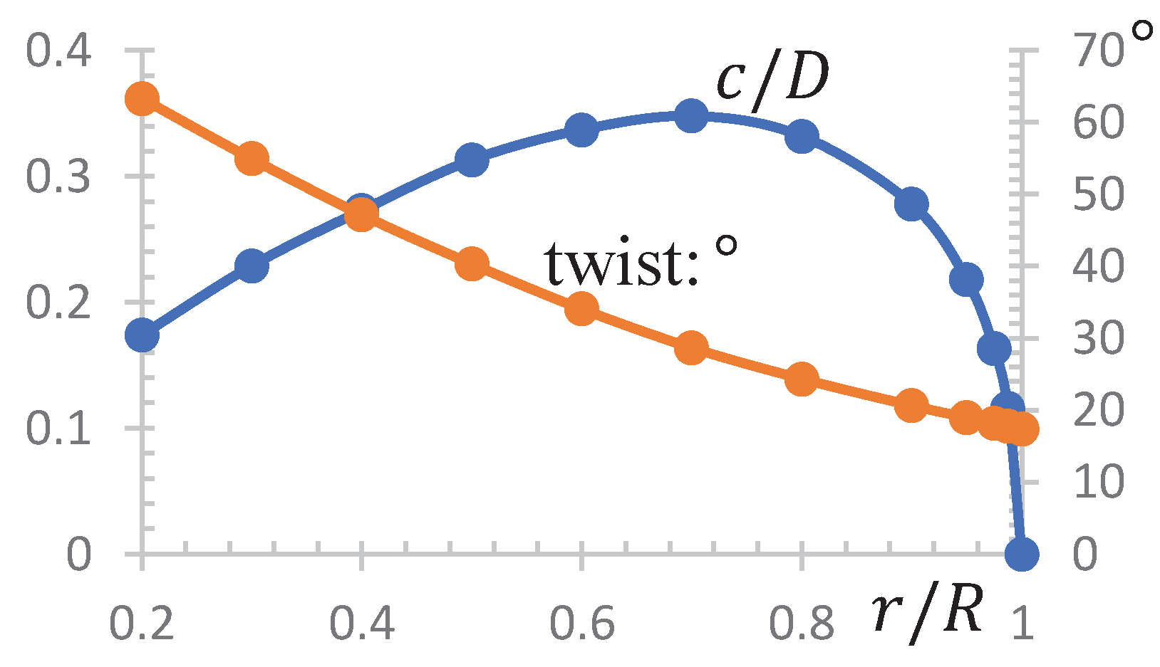
This study used a five bladed, right-handed, variable pitch, non skew, and no rake marine propeller DTMB 4381, as used in Bridges [29]. Cylindrical cross-sections of the blade at $r/R=0.2\sim 1$ are airfoils as shown in Figure 1, in which R is the radius of the propeller rotor disc. The distributions of relative chord length (normalized with propeller diameter D) and twist angle are shown in Figure 2. The hub was tapered.

The forces and moments of a specific geometric propeller can be represented by a series of dimensionless quantities [30], including thrust coefficient $K_T$, torque coefficient $K_Q$, advance coefficient (also called advance ratio) J and cavitation number $\sigma$, they are

$$K_T=\frac{T}{\rho n^2{D}^4},K_Q=\frac{Q}{\rho n^2{D}^5},J=\frac{V_a}{nD},\sigma =\frac{p_0-e}{\rho V^2/2}$$

(39)

where, e is water vapor saturation pressure. The dimensional analysis method can be used to analyze geometrically similar propellers. When a marine propeller operates far from the free water surface and does not cause surface waves, the forces acting on it are easily understood to be related to the diameter D, the advance speed $V_a$, the rotational speed n, the density of the fluid $\rho$, the viscosity of the fluid $\mu$ and the static pressure of the fluid at the propeller $(p_0-e)$. Therefore, the thrust T on the propeller is proportional to them, i.e., $T\propto {\rho }^{k_1}{D}^{k_2}{V}_a^{k_3}{n}^{k_4}{\mu }^{k_5}{(p_0-e)}^{k_6}$. To ensure that the dimensions on both sides of the equation are the same, we can obtain $\left(ML\right)/T^2={(M/L^3)}^{k_1}{L}^{k_2}{(L/T)}^{k_3}{(1/T)}^{k_4}{(M/\left(LT\right))}^{k_5}{(M/\left(L{T}^2\right))}^{k_6}$, with the mass M, the length L and the time T. Compare the left and right ends of this equation to get $1=k_1+k_5+k_6$ for M, $1=-3k_1+k_2+k_3-k_5-k_6$ for L and $-2=-k_3-k_4-k_5-2k_6$ for T, then we get $k_1=1-k_5-k_6,k_2=4-k_3-2k_5-2k_6$ and $k_4=2-k_3-k_5-2k_6$, which used to get $T\propto {\rho }^{(1-k_5-k_6)}{D}^{(4-k_3-2k_5-2k_6)}{V}_a^{k_3}{n}^{(2-k_3-k_5-2k_6)}{\mu }^{k_5}{(p_0-e)}^{k_6}$, then $T\propto \rho n^2{D}^4{(V_a/\left(nD\right))}^{k_3}·{(\mu /\left(\rho n{D}^2\right))}^{k_5}·{((p_0-e)/\left(\rho n^2{D}^2\right))}^{k_6}$, so

$$K_T=J^{k_3}{\left(\frac{1}{Rn}\right)}^{k_5}{\sigma }_0^{k_6}=f(J,Rn,{\sigma }_0),R_n=\frac{\rho n{D}^2}{\mu },{\sigma }_0=\frac{p_0-e}{\rho n^2{D}^4}$$

(40)

In the same way we also have $K_Q=g(J,Rn,{\sigma }_0)$. The open water efficiency of a propeller is defined as the ratio of thrust horsepower to delivered horse power as

$${\eta }_0=\frac{T{V}_a}{2\pi nQ}=\frac{K_T}{K_Q}\frac{J}{2\pi }$$

(41)

Let $P_B$ the brake power or the maximum continuous rating power which is delivered at the engine coupling flywheel, then the shaft power $P_S$ at the output coupling of the gearbox is $P_S=P_B{\eta }_1$ with $96\%\le {\eta }_1\le 98\%$. The power transmitted to the propeller and absorbed by the propeller is defined as the increase in kinetic energy per unit time of the slipstream or the work done by the propeller thrust after deducting the loss of bearings, i.e., $P_D=P_S{\eta }_S=2\pi nQ$ with $98\%\le {\eta }_S\le 99\%$, in which the shafting mechanical efficiency ${\eta }_S$ is usually between 98% and 99% depending on the length of the shaft and the number of bearings. Another definition of thrust and power coefficient is

$$C_T=\frac{T}{\rho A{V}_a^2/2},C_P=\frac{P_D}{\rho A{V}_a^3/2}$$

(42)

with the disc area $A=\pi R^2$. International Towing Tank Conference (ITTC,1978) report another Reynolds number $R{e}_c=(c_{0.75}{\sqrt{V^2}}_a+{\left(0.75\pi nD\right)}^2)/\nu$ with $c_{0.75}$ the chord length at $r=0.75R$ of the propeller.

2.4. Computational Domain and Meshing

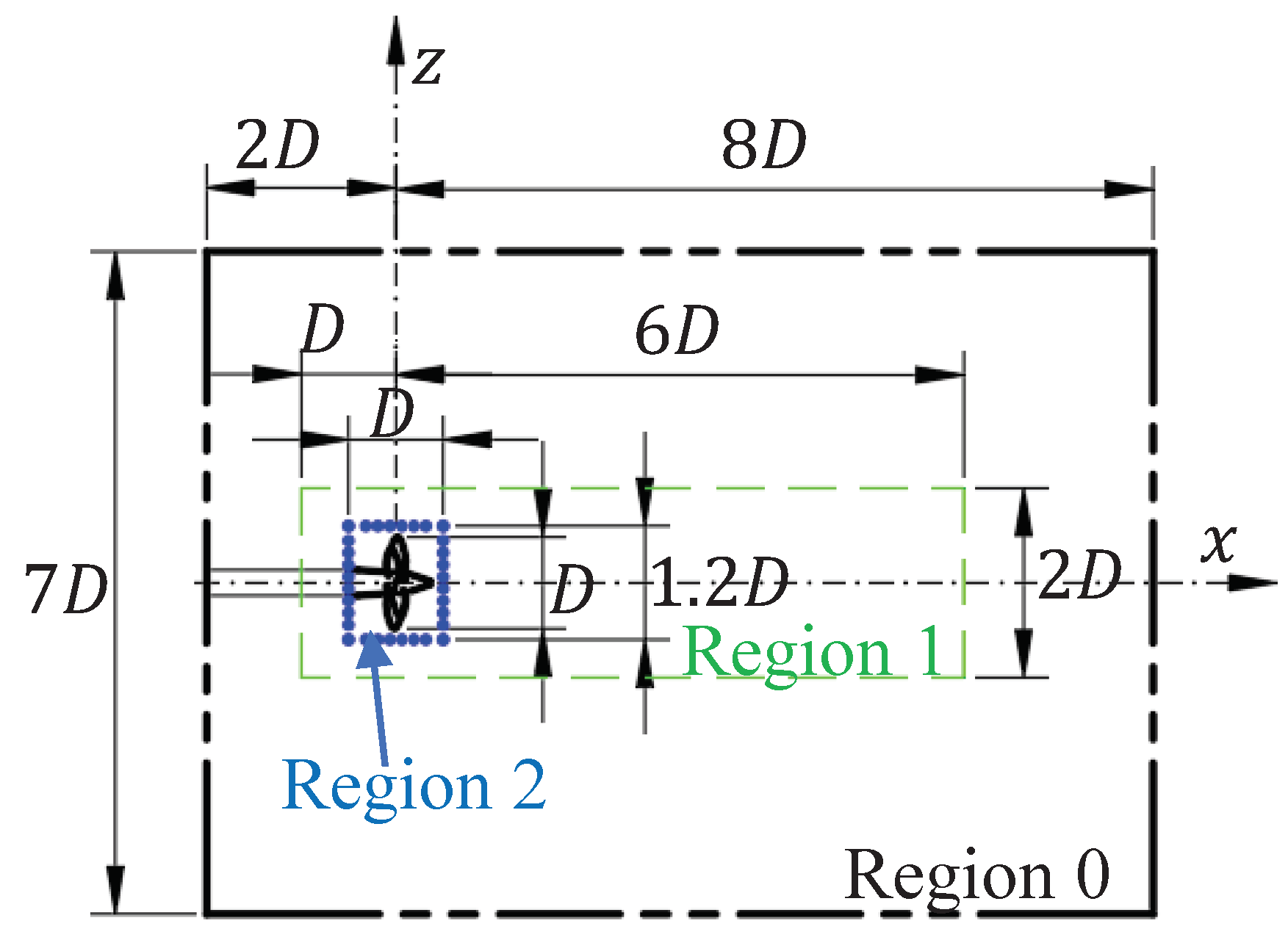
To avoid blocking effects [31] caused by setting the computational domain too small, set the right-hand reference coordinate system and arrange the computational domain as shown in Figure 3. The outer boundary of the flow field, namely the water channel, is a cylinder with a diameter of $7D$ and a height of $10D$. The center of propeller blades is at the origin and the flow direction is in the positive direction of the x-axis. The computational domain spans between $2D$ upstream and $8D$ downstream of the propeller. The channel blocking factor for this arrangement is about 0.021 (less than 0.1), where the blocking factor of the channel is defined as $ϵ=A/A_c$ with A the disc area of propeller and $A_c$ the area of water tunnel cross-section. The simulations are performed using unstructured grids with about 8.5 million hexahedral cells for LES-LDKSGS and RANS-kEpsilon (also with different refinements). Views of overall mesh distribution are shown in Figure 4. Grid refinement is performed in the wake zone of the propeller to capture the small-scale structures of interest to us. The grid scale size in different regions in Figure 3 is shown in

Table 2. Grid size in different regions of the computational domain.

Region	Cell Scales: (with about Total 8.5 Million Cells)
Region 0 (double-dashed line)	0.125D
Region 1 (dashed line)	0.015625D
Region 2 (dotted line)	0.0078125D

. The time step for LES numerical simulation is set to ${10}^{-5}$s, and the time taken for the propeller to rotate one cycle at the designed advance ratio $J=0.889$ is equivalent to 3956 calculation time steps, and at J = 313,350 calculation time steps.

Considering the computational cost, LES-LDKSGS simulation was only performed on approximately 8.5 million grids with $J=0.889$ and $J=3$. In order to compare and illustrate, we also intentionally performed simulations on about 8.5 million, 3.07 million, 1.15 million and 38,000 grids for RANS-kEpsilon at different advance ratios, although there is no need for such fine mesh (such as 8.5 million) in RANS-kEpsilon simulation with a good grid strategy. All 42 simulations included in this paper are listed in

Table 3. Grid size in different regions of the computational domain.

Case	Turbulent Model	Advance Coefficient J	Number of Grids
Case 1	LES-LDKSGS	0.889	∼8.5 million
Case 2	LES-LDKSGS	3	∼8.5 million
Case 3	RANS-kEpsilon	0.889	∼8.5 million
Case 4	RANS-kEpsilon	0.889	∼3.07 million
Case 5	RANS-kEpsilon	0.889	∼1.15 million
Case 6	RANS-kEpsilon	0.889	∼38,000
Case 7–24	RANS-kEpsilon	0.1, 0.2, 0.3, 0.4, 0.5, 0.6, 0.7, 0.8, 0.9, 1, 2, 3, 4, −0.1, −1, −2, −3, −4 (1)	∼38,000 grid cells
Case 25–32	RANS-kEpsilon	−1, −2, −3, −4, 1, 2, 3, 4 (1)	∼38,000
Case 33–42	RANS-kEpsilon	0.1, 0.2, 0.3, 0.4, 0.5, 0.6, 0.7, 0.8, 0.9, 1 (2)	∼38,000

⁽¹⁾ with $U_x$ = −4.4945 m/s. ⁽²⁾ with n = 25 r/s.

.

2.5. Initial and Boundary Conditions

As shown in Figure 5, boundary conditions are specified. Free-stream velocity boundary conditions are specified at the inlet; no-slip boundary condition at the lateral boundaries to simulate the real tunnel; convective boundary conditions are prescribed at the outlet; boundary conditions on the blades and hub are rotating walls; boundary condition on shaft is specified as no-slip BCs. All sampling points used in this paper are also shown in Figure 5 using horizontal dashed lines and vertical double-dashed lines, that is

• Position of horizontal dashed lines: $r/R$ = 0.7, 0.8, 0.9, 1, 1.1, 1.2, 1.3, 1.5, 2, 3, 4, 5, 6.;
• Position of vertical double-dashed lines: $x/D=-1.8,-1,-0.5$, 0.06, 0.08, 0.1, 0.115, 0.5, 1, 2, 3, 4, 5, 6, 7, 7.8.

2.6. Numerical Method

Use unstructured mesh finite volume method for numerical calculations, and use numerical altorithms to solve partial differential equations (PDE). The semi-implicit method for pressure-linked equations method (SIMPLE) [32,33] widely known in the engineering literature is perhaps the oldest and most widely used iterative method for the stationary N-S equations. For unsteady N-S equations we use pressure implicit with splitting of operators (PISO) method [34], which is a variant of SIMPLE. In PISO method which is a predictor-corrector approach, we take the small-time-step assumption so that the pressure and velocity coupling is much stronger than the nonlinear coupling. Then the nonlinear term can be linearized and the velocity field can be explicitly corrected, while the discretization of the momentum equation is safely frozen. The solver is set up on the platform of OpenFOAM [35] and mainly includes two steps: the momentum prediction and the pressure correction.

Firstly, calculate the velocity at the center of the cell, and then interpolate its value to the center of the cell surface, which is called the flux. Then project the flux to ensure that the pressure Poisson discrete equation is satisfied. Using a multigrid approach to iteratively solve the Poisson equation, the obtained pressure value is used to update the predicted velocity field. Time discretization using a second order implicit Crank-Nicolson bounded scheme. The standard finite volume discretization of Gaussian integral is used for spatial discretization, and linear interpolation is used for the value from the center of the cell to the center of the face. And limiting the gradient so that when the calculated gradient is used to extrapolate the cell value to the face, the face value will not exceed the range of values in the surrounding cells, thus ensuring boundedness. In order to maintain the second-order accuracy, explicit non orthogonal correction is taken for non orthogonality grids. The pressure Poisson equation is solved using the geometric aggregated algebraic multi-grid (GAAM) method.

3. Verification and Comparison

3.1. Verification of Adequate Domain Size

The propeller wake is influenced by the size of the computational domain, so the computational domain setting must be large enough to reduce channel blockage effects. As a rule of thumb, if the blockage (defined as the ratio of two areas of propeller disk and domain cross section) less than 0.1, the rotor wake can be deemed unconfined and effects of finite domain size are negligible. This verification is clearly shown in Figure 6. At $r/R=6$, the perturbation of axial velocity is less than 1% and can be basically ignored. At $x/D=-1.8$ upstream of the propeller, the radial variation in axial velocity can also be ignored. Taking into account the axial symmetry of the five-blade propeller, the figure shows the normalized mean value of sampling points of every 9° within an angle of 72°. From the results we can conclude that the present choice of domain size is proper and adequate. From the results, we can conclude that the selection of domain size is appropriate and sufficiently large, and its impact on the evolution of propeller wake can be ignored.

3.2. Mean Force Comparison

Mean non-dimensional thrust coefficient $\langle K_T\rangle$ and torque coefficient $\langle K_Q\rangle$ of LES-LDKSGS model, RANS-kEpsilon model and LES-GASGS model are compared with the three physical experiment results, as shown in

Table 4. Mean thrust and torque coefficients.

Experiment	$\mathit{Re}$	${\mathit{Re}}_{\mathit{c}}$	$\langle {\mathit{K}}_{\mathit{T}}\rangle$	Relative Error (${\mathit{e}}_1,{\mathit{e}}_2,{\mathit{e}}_3$)% *	$\langle {\mathit{K}}_{\mathit{Q}}\rangle$	Relative Error (${\mathit{e}}_1,{\mathit{e}}_2,{\mathit{e}}_3$)% *
LES-LDKSGS (case1)	$8.9\times {10}^5$	$8.3\times {10}^5$	−0.201	(0.0, 11.6, 4.7)	0.041	(2.6, 7.8, 2.3)
RANS-kEpsilon (case3)	$8.9\times {10}^5$	$8.3\times {10}^5$	−0.194	(3.5, 7.8, 8.1)	0.042	(0.2, 10.5, 0.0)
LES-DASGS [3]	$8.9\times {10}^5$	$8.3\times {10}^5$	−0.21	(4.5, 16.7, 0.5)	0.041	(2.6, 7.8, 2.3)
OW (Jessup et al., 2004)	$1.1\times {10}^6$	$1.02\times {10}^6$	−0.201	-	0.0421	-
WT (Jessup et al., 2006)	$8.9\times {10}^5$	$8.3\times {10}^5$	−0.18	-	0.038	-
OW (Hecker and Remmers, 1971)	$6.47\times {10}^5$	$6\times {10}^5$	−0.211	-	0.042	-

* $e_1,e_2,e_3$ respectively correspond to the errors relative to WT, OW2006, and OW1971.

. For physical experiments, both mean thrust and torque coefficients in the water tunnel (WT) are slightly smaller than in the open water towing tank (OW), possibly due to tunnel blocking effects. LES-LDKSGS results show good agreements with the WT (Jessup et al. 2006) results, but less than RANS-kEpsilon results under the same refinement, which implies that if your concern is only for mean force of the propeller the LES method may be not your best choice considering cost. The results of LES-LDKSGS with a lower computational cost is more accurate than the results of LES-DASGS, which shows the superiority of the LES-LDKSGS model to some extent.

3.3. Compare with PIV Data

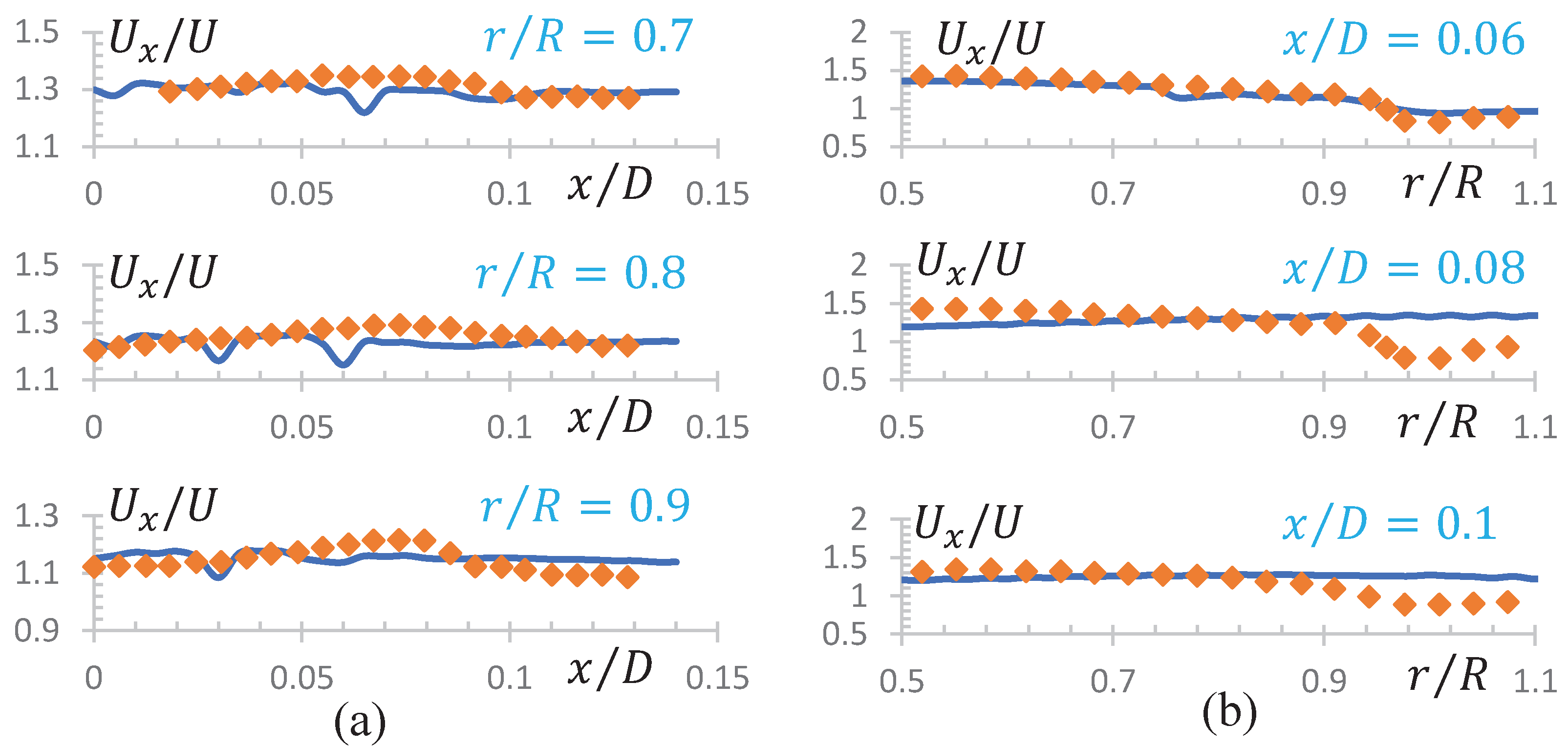
The comparison between LES-LDKSGS simulation results and PIV measurement values (Chang, P. & Marquardt, M., 2016, reproduce from [3]) of the phase average axial velocity profile at streamwise position $x/D$ = 0.06, 0.08, 0.1 and radial location $r/R$ = 0.7, 0.8, 0.9, is shown in Figure 7. The values are normalized with free stream velocity. It can be seen that at these locations in the near field, the two results are basically consistent, except that the flow downstream of the blade tip region is smoothed faster than the measured results of PIV.

3.4. Compare with Different Advance Ratios

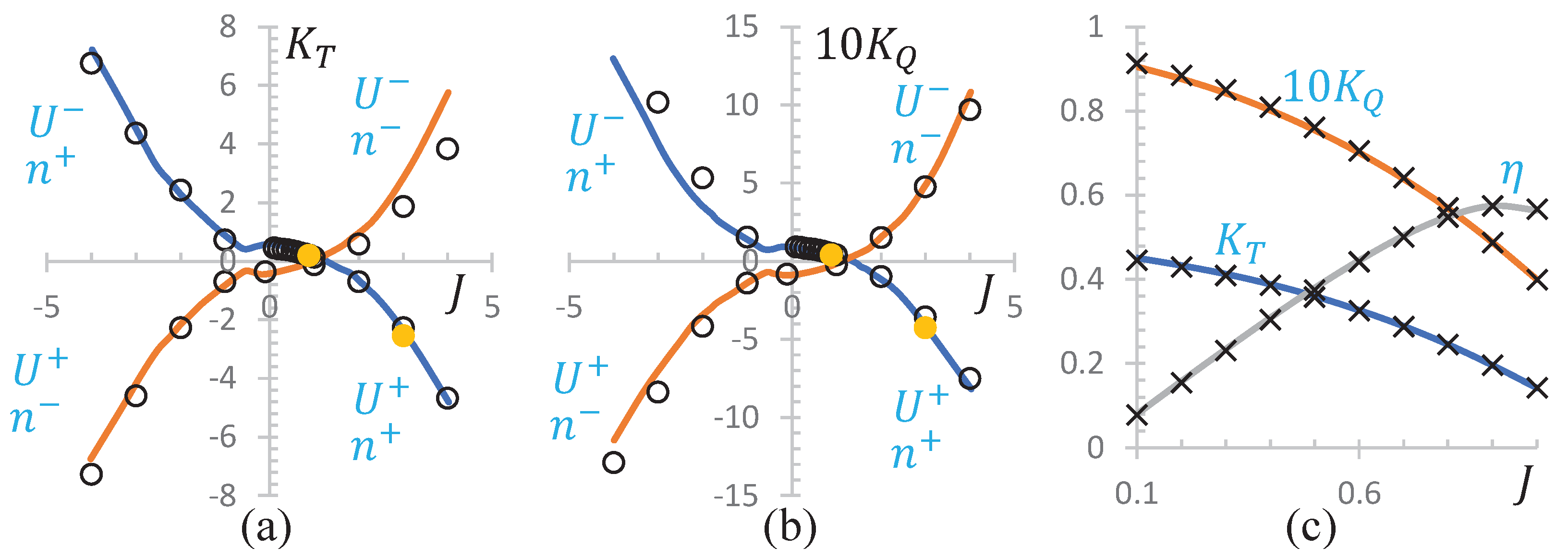
The thrust coefficient and ten times the torque coefficient with different turbulent models under the deliberately selected J (avoid excessive numerical simulations) are compared with open-water data from Hecker and Remmers (1971), which are shown in Figure 8a,b. Both the LES-LDKSGS model and the RANS-kEpsilon model get results that are in line with the physical experiment. However, the LES model requires a higher calculation cost than the RANS model, so the LES model has no advantage in calculating the average thrust and torque of the propeller as already stated. Coefficients of thrust, torque and efficiency at uniform inlet velocity $U_x$ = 4.4945 m/s and at constant rotating speed n = 25 r/s for different advance ratios $J\in [0.1,1]$ are shown in Figure 8c. The difference of them is due to the different Reynold numbers. As the $Re$ increases, the gap between them becomes smaller. There is a critical Reynolds number, when the actual Reynolds number exceeds this value, the influence of different Reynolds numbers can be ignored.

4. Results and Discussion

4.1. Time History of Force

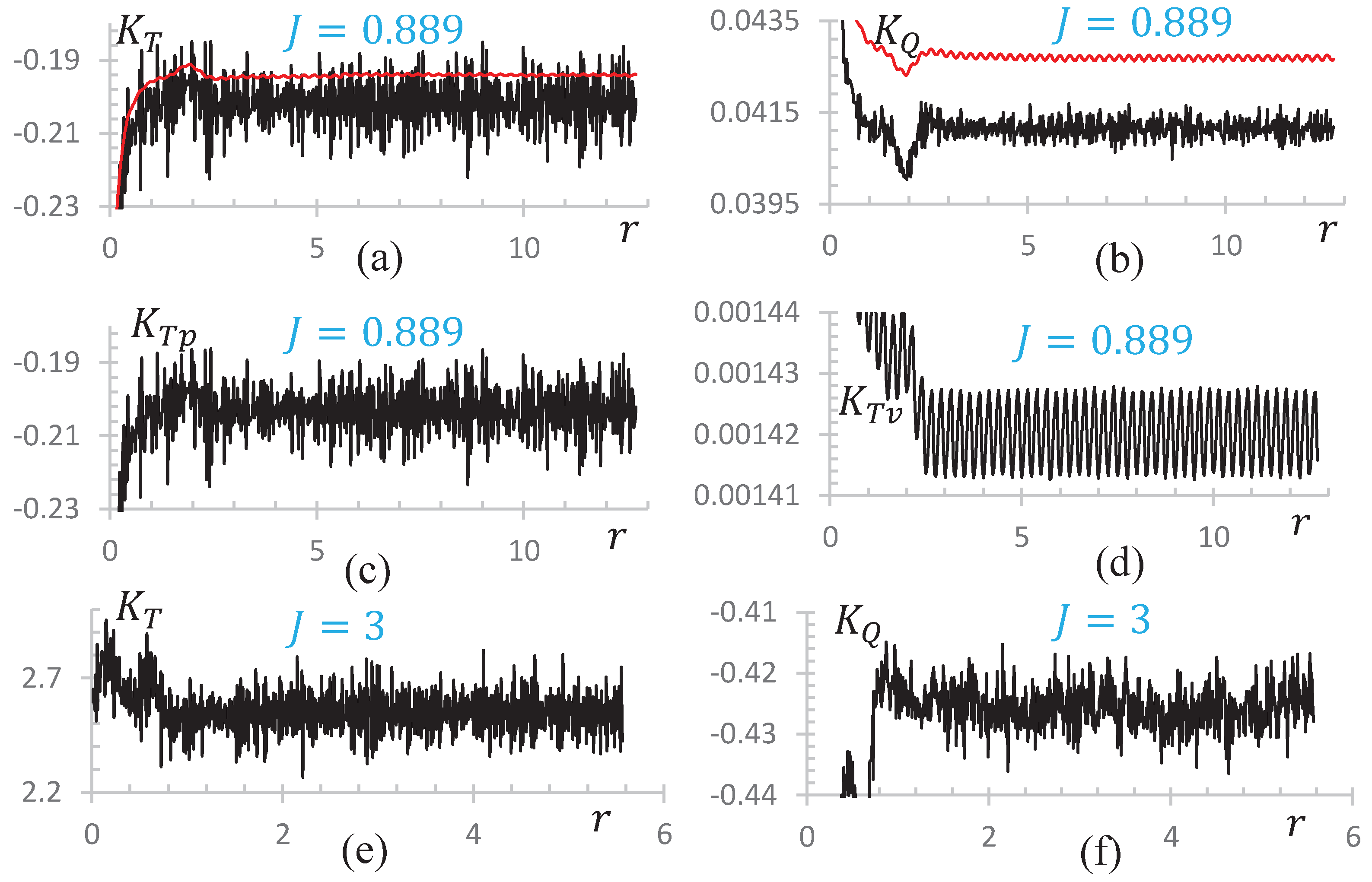
The time history results of thrust and torque coefficients at the design advance ratio are shown in Figure 9a,b. The force on propeller basically tends to a stable mode after about 3 revolutions. After about 10 revolutions, the changes of average thrust and torque are very small and can be ignored. At this time, the wake of the propeller can be considered stable periodically. The physical quantity after the tenth turn is used for phase average calculation. Obviously it can be seen that the force perturbation of the LES-LDKSGS model (black line) is much stronger than that of the RANS-kEpsilon model (red line). Note that the thrust coefficient of the propeller here is negative, indicating that the thrust direction is negative along the x-axis. The torque of the propeller is positive, indicating that its direction points towards the positive direction of the x-axis determined by the right-hand rule, which is opposite to the direction of the propeller’s rotation. This part of the propeller torque is directly related to the selection of the engine that drives the shaft to rotate, which is very important in engineering applications. The pressure and viscous force components of the propeller are shown in Figure 9c,d, and the pressure force is two orders of magnitude higher than the viscous force. The thrust and torque coefficients at non-design advance ratio are shown in Figure 9e,f, which shows a wider perturbation band compared to the results at design conditions.

4.2. PSD of Force

For any time signal $x\left(t\right)$, this signal can be any physical quantity that changes with time.When analyzing the energy of the signal, it is regarded as the unit resistance applied to the resistance, that is, R = 1 $\Omega$. The current acts on the resistor. Based on this, the energy attribute of this unit resistance is regarded as the energy attribute of this signal. Therefore, the total energy of this signal is

$$E=\underset{T\to \infty }{lim}{\int }_{-T}^T{I}^{2}Rdt=\underset{T\to \infty }{lim}{\int }_{-T}^T{x}^2\left(t\right)dt$$

(43)

At the same time, energy can also be expressed in the frequency domain as

$$E=\frac{1}{2\pi }{\int }_{-\infty }^{\infty }{\left|X\left(\omega \right)\right|}^{2}d\omega withX\left(\omega \right)={\int }_{-\infty }^{\infty }x\left(t\right)e^{-j\omega t}dt$$

(44)

called the Fourier transform or spectral function of $x\left(t\right)$. And the average power of the signal is

$$P=\underset{T\to \infty }{lim}\frac{1}{2T}{\int }_{-T}^T{x}^2\left(t\right)dt$$

(45)

Of course, for different signals, the limits in the above two definitions do not necessarily exist, so energy signals and power signals can be distinguished. In other words, if the first limit exists, it is called an energy signal, and if the second limit exists, it is called a power signal. A signal can be neither an energy signal nor a power signal, but it cannot be both an energy signal and a power signal. In many engineering and technical problems, it is necessary to calculate the power spectrum of a time series, which is defined as the square of the absolute value of the spectral function. The calculation of the power spectrum follows the following steps:

• Step1: cut off a tail or add some $0s$ to the original data to make the sequence length $N=2^m$, then the time series $f\left(t\right)$ is given as discrete samples $f_j=f(j\Delta t);j=0,1,\cdots ,N-1$;
• Step2: use the appropriate “data window” $g(t/T)$ to correct $f_j$, i.e., $u_j=f_j{g}_j$;
• Step3: fast algorithm to calculate the discrete Fourier transform $U_k$ of the sequence of real numbers $u_j$, that is $U_k={\sum }_{j=0}^{N-1}{u}_j{W}_N^{-jk};k=0,1,\cdots ,N-1$;
• Step4: get power spectrum estimate $P(k\Delta s)\simeq \frac{2\Delta t}{N}{\left|U_K\right|}^2;k=0,1,\cdots ,\frac{N}{2}$ where $\Delta s=1/T$ and $T=N\Delta t$.

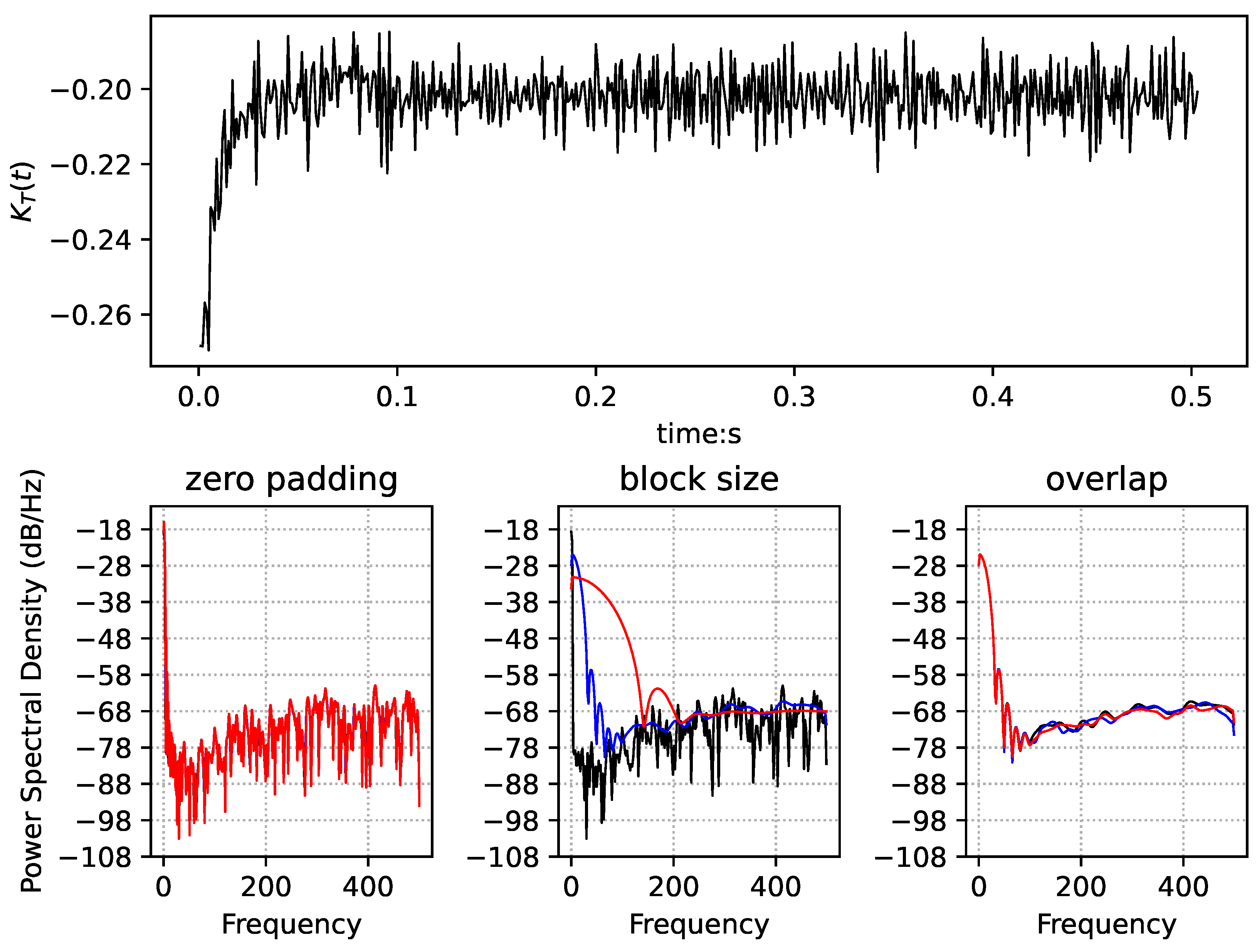
The power spectral density (PSD) of $K_T$ is shown in Figure 10.

4.3. Circulation

The circumferentially averaged azimuthal velocity ${\overline{U}}_{\theta }\left(r\right)$ at downstream $x=0.12D$ of the propeller is shown in Figure 11, which is defined as

$$G\left(r\right)=\frac{r{\overline{U}}_{\theta }\left(r\right)}{Z}$$

(46)

here Z is the number of blades with a value of 5. The radial distribution of average loading can be represented by this circulation $G\left(r\right)$ to some extent. From Figure 11, it can be seen that the load at the tip of the propeller blade is relatively mild, while the relatively high load near the tip can lead to strong and large tip vortices. The strength of the vortex shedding from the trailing edge of the blade is directly related to the radial gradient of the circulation near the blade cross-section. The propeller in this article exhibits strong blade trailing edge vortex shedding under the design condition, which is different from propellers with heavy blade tip loads.

4.4. Instantaneous

The instantaneous contours of normalized velocity components $U_x/U$, $U_y/U$ and $U_z/U$ in the $xy$ plane are shown in Figure 12a. The near field wake of the propeller is mainly composed of coherent blade tip vortices and blade trailing edge vortices, which gradually become unstable and break in the far field. The axial velocity cloud maps at 15 locations ($x/D$ = −0.1, −0.08, −0.06, 0.06, 0.08, 0.1, 0.5, 1, 2, 3, 4, 5, 6, 7, 7.8) in the flow direction are presented on the transverse planes, as shown in Figure 12b. The mutual induction of blade tip vortices and rolled-up blade trailing edge vortices dominates the evolution process of propeller wake from near field to far field, and the actual evolution mechanism depends on the geometry and operating conditions of the propeller.

4.5. Mean Axial Velocity Profiles

The azimuthal-averaged profile of relative axial velocity at twelve locations $x/D=2,-1.8,-1,-0.5,0.5,1,3,4,5,6,7,7.8$ are shown in Figure 13 respectively for results of LES-LDKSGS (black solid line), LES-DASGS (black dashed line, only at $x/D=2$) and RANS-kEpsilon models with different refinements (red solid line is more refined than red dashed line). For the sake of simplification, the result of LES-LDKSGS model are given only at $x/D=2$. Note that the number of grids in LES-DASGS simulation is much higher than in LES-LDKSGS simulation. The LES-DASGS simulation uses about 181 million grid cells and the LES-LDKSGS simulation uses about 8.5 million grid cells. However, the results of the two different large eddy simulations (LES-LDKSGS and LES-DASGS) are very close. That is to say, we get basically the same result with less computational cost. To some extent, this also shows the superiority of the method LES-LDKSGS. The results of RANS-kEpsilon are obviously different from those of LES-LDKSGS, even when the same refinement is used. It is obvious that the RANS-kEpsilon model has a smooth effect on the wake and shows more axial velocity dissipation. The result of the RANS-kEpsilon model tend to be closer to the results of LES-LDKSGS model with the increase of refinement in the near field from about $x=-1.8D$ to $x=2D$, but the opposite situation does occur about $x\ge 2D$ downstream of the far field. This result has important practical significance, that is, when we do not pay attention to the near field, in the RANS simulations, it may not be necessarily true that the denser the grid, the better the calculation results.

4.6. Mean Square Velocity Fluctuations

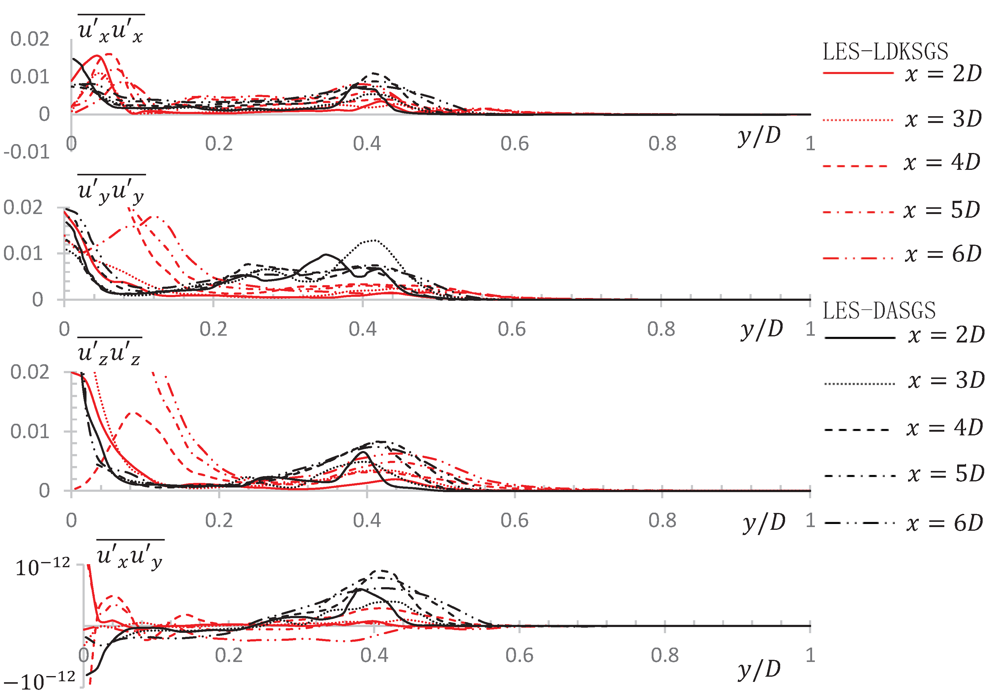
After calculating the periodic stability, the velocity field is averaged, and the velocity perturbation of the rotating propeller for one cycle is calculated based on the average velocity value.The azimuthal-averaged perturbations of mean square velocity in different directions are shown in Figure 14. The results of LES-LDKSGS (case1) and LES-DASGS are shown in the figure for comparison. The two are basically consistent in terms of magnitude, only showing certain differences in the central area of the propeller hub. Given the differences in calculation settings between the two, this error can be ignored to a certain extent, and it can be said that the calculation of flow field effects between the two is similar.

4.7. Vortex Structures

Since the coherent structures (CS) in turbulence has been widely regarded as vortices, the question of what constitutes vortices in turbulence has become meaningful. The objective definition of vortices should allow the use of the concept of vortex dynamics to induce CS, and be able to use CS to explain the formation and evolution of vortices in turbulent phenomena. CS can also be used to develop various turbulence models and control strategies for turbulent phenomena [36]. Intuitively, a vortex is considered a flow tube, with its surface composed of vortex lines [37]. However, the existence of vortex tubes cannot represent the existence of vortices, such as vortex tubes in laminar pipe flow, which are not vortices in any sense. Lugt (1979) defined a vortex as multiple particles of matter rotating around a common center, Chong et al. (1990) as a region of complex eigenvalues of $\nabla \mathit{u}$, Hunt et al. (1988) as a region containing both a positive second invariant of $\nabla \mathit{u}$ and low pressure, and Jinhee and Fazle [36] defined it in terms of the eigenvalues of the symmetric tensor (${\mathit{S}}^2+{\Omega }^2$), in which $\mathit{S}$ and $\Omega$ are symmetrical and asymmetrical parts of the velocity gradient tensor $\nabla \mathit{u}$. Robinson (1991) used the DNS database in 1991 to draw a conclusion that the low-pressure criterion can effectively capture the vortex structure in the turbulent boundary layer, but in more general cases, it is not possible to clearly give a certain pressure level to identify all vortex regions in the flow. Therefore, a single pressure threshold cannot reveal all phenomena. The methods of vortex identification available are listed in

Table 5. Vortex identification technology.

No.	Criterion for Vortex Identification
1	Local pressure minimum
2	Pathline and streamline
3	Vorticity magnitude
4	Existence of complex eigenvalues of $\nabla \mathit{u}$
5	Second invariant Q of $\nabla \mathit{u}$ and kinematic vorticity number $N_k$
6	Eigenvalues (${\lambda }_1>{\lambda }_2>{\lambda }_3$) of (${\mathit{S}}^2+{\Omega }^2$)

.

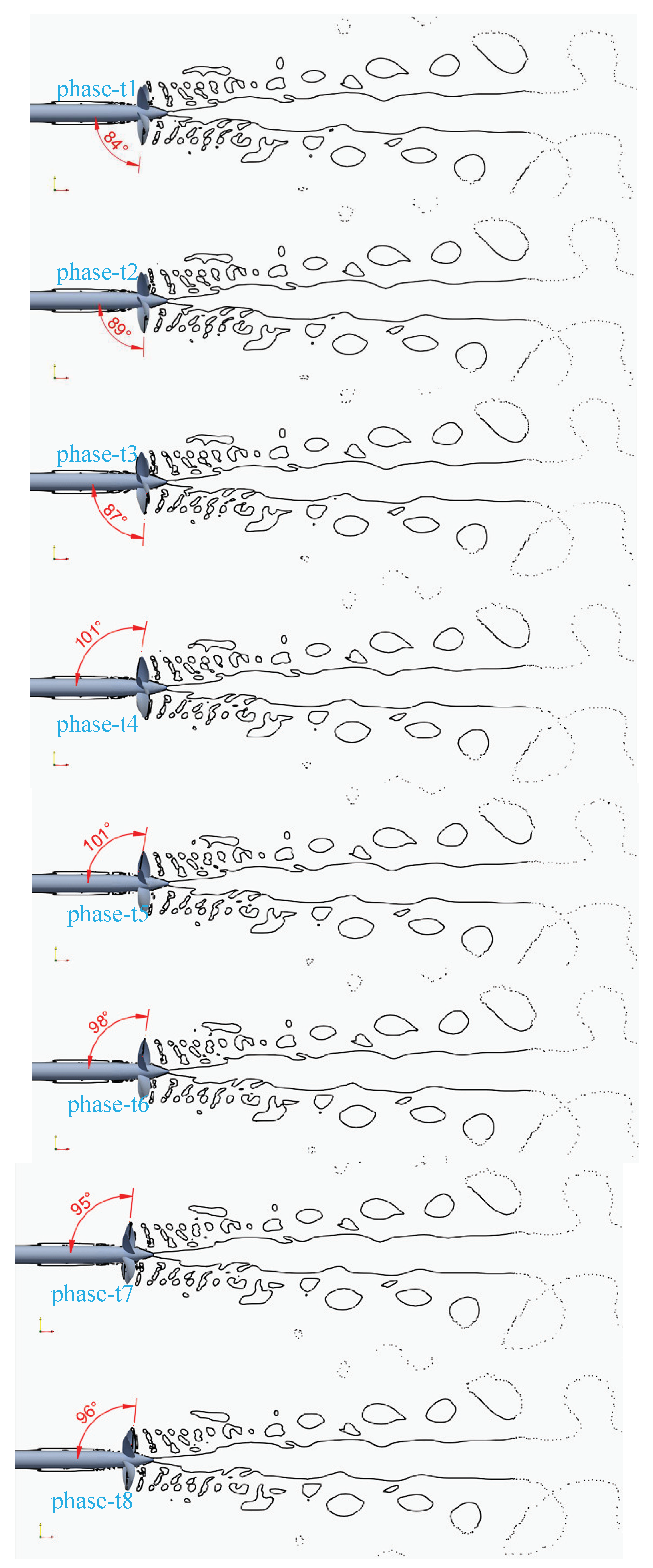
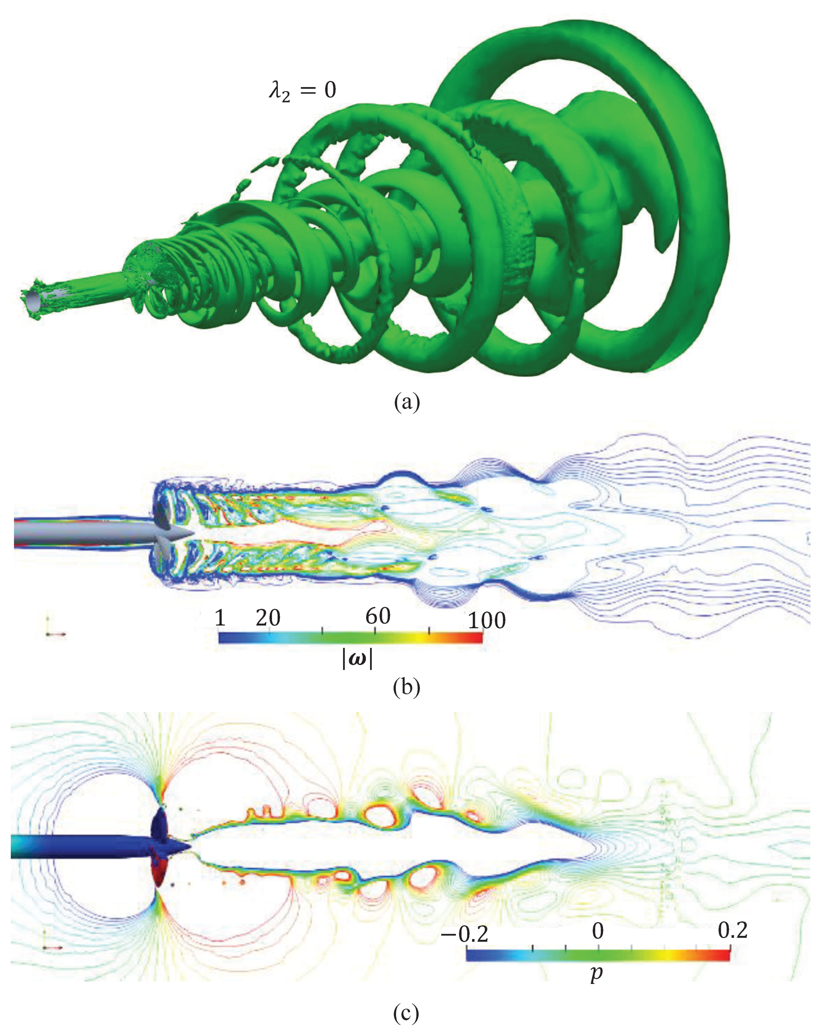
The size of vortices in viscous fluids depends on the selected standard threshold. We can identify the vortex core, and the necessary condition for its existence is that there is a net vorticity and the geometry of the vortex core is Galilean invariant. These two necessary conditions cannot lead to a definite identification method, and can only serve as a prerequisite for the possible existence of vortices. Jinhee and Fazle [36] attempted to develop an objective method for identifying vortex core in any flow. Figure 15 and Figure 16 show the CS of vortices in propeller wake under different criterions. The iso-contour of ${\lambda }_2=0$ is shown in Figure 15. Since it is a 5-blade propeller, Figure 15 only shows the instantaneous planes of 8 successive time units within one phase angle (${72}^{\circ }$) respectively from top to bottom. The vortex area angle on the blade surface has been marked red on the figure, and the angle increases first and then decreases. Other phase angles have similar results and will not be repeated for simplicity. It can be clearly seen that the interaction between tip vortex helix and trailing edge vortex becomes blurred after about $1D$ downstream of the propeller. After $2D$, hub vortex, blade tip vortex and trailing edge vortex meet to further blur the wake. In the near field of wake, some vortex cores with small radius are mainly formed, and the diameter of vortex core increases in the far field. The vortex core radius at the center of the propeller shaft increases more downstream. Figure 16a shows a 3D axis side view of ${\lambda }_2=0$, and Figure 16b,c are iso-contours of vorticity magnitude and pressure. It is obvious that the pressure criterion is insufficient.

5. Summary and Conclusions

In the framework of continuum mechanics, assuming that the fluid is single-phase incompressible Newtonian fluid with uniform constant density water, the flow through a marine propeller is studied in physical space by solving general N-S equations and using local dynamic k-equation subgrid-scale model LES-LDKSGS according to different space-time resolution and dynamic description levels. If the commutation error generated by the differentiation of the filter applied in space can be ignored, then the filtered momentum equation introduces a nonlinear term that can be represented by a subgrid tensor. This nonlinear term can be decomposed, and based on the separability assumption of turbulence at large and small scales, direct simulation calculations can be carried out for anisotropic large scales with high energy in turbulence, while turbulence at small scales is modeled using the SGS model. The small-scale turbulence perturbations are modeled through eddy viscosity and diffusivity assumptions, which are themselves smoothed out in the flow.

Within the applicable scope of the self-similarity hypothesis, when a dynamic k-equation SGS model is used to close the general N-S equations for flow, the LES-DKSGS model is obtained, and this model does not assume the local balance of SGS energy generation and dissipation, but directly simulates and calculates SGS to account for the nonlocal and historical effects completely ignored by the LES-DASGS model. Therefore, it can be optimistically expected that the LES-DKSGS model will provide better vortex viscosity predictions than the LES-DASGS model. However, in order to avoid numerical instability, the LES-DKSGS model adopts a local averaging technique for model coefficient calculation, which also has certain drawbacks. Using a local dynamic k-equation model (LES-LDKSGS), as no averaging technique is introduced in the calculation of model coefficients, vortex viscosity predictions can be directly calculated locally and does not cause numerical instability.

The wake of a five-bladed, right-handed marine propeller with variable pitch, no skew and no rake was studied. There are all 42 simulations included in this paper. From these numerical experiments, we mainly draw the following conclusions:

• For mean thrust and torque coefficients LES-LDKSGS (used in our article) results show good agreements with the WT (Jessup et al. 2006) results, but less than RANS-kEpsilon results (using the same mesh as in LES-LDKSGS simulation, note there is actually no need of too refinement grid for RANS-kEpsilon simulation) under the same computing cost, which implies that if your concern is only for mean force of the propeller the LES method may be not your best choice considering cost;
• The results of LES-LDKSGS (used in our article) with a lower computational cost is comparable to the results of LES-DASGS [3], which shows the superiority of the LES-LDKSGS model than the LES-DASGS model to some extent;
• The evolution mechanism of propeller wake is well captured by the LES-LDKSGS model, including the interaction mechanism between the tip vortex and the trailing edge vortex that dominate the evolution of propeller wake from near to far fields, although this mechanism actually depends on the geometry and operating conditions of the propeller;
• The vortex CSs of the propeller wake, including the size of the vortex core, are visualized using different criterions to give more insight.

References

1. Posa, A.; Broglia, R.; Felli, M.; Cianferra, M.; Armenio, V. Hydroacoustic analysis of a marine propeller using large-eddy simulation and acoustic analogy. J. Fluid Mech. 2022, 947, A46-1. [Google Scholar] [CrossRef]
2. Nicoud, F.; Ducros, F. Subgrid-scale stress modelling based on the square of the velocity gradient tensor. Flow Turbul. Combust. 1999, 62, 183–200. [Google Scholar] [CrossRef]
3. Kumar, P.; Mahesh, K. Large eddy simulation of propeller wake instabilities. J. Fluid Mech. 2017, 814, 361–396. [Google Scholar] [CrossRef]
4. Hyunchul, J.; Krishnan, M. Large eddy simulation of flow around a reverse rotating propeller. J. Fluid Mech. 2013, 729, 151–179. [Google Scholar]
5. Germano, M.; Piomelli, U.; Moin, P.; Cabot, W.H. A dynamic subgrid-scale eddy viscosity model. Phys. Fluids A 1991, 3, 1760. [Google Scholar] [CrossRef]
6. Lilly, D.K. A proposed modification of the Germano subgrid-scale closure method. Phys. Fluids A Fluid Dyn. 1992, 4, 633. [Google Scholar] [CrossRef]
7. Martin, V.; Krishnan, M. Large eddy simulation of crashback in marine propellers. In Proceedings of the 44th AIAA Aerospace Sciences Meeting and Exhibit, Reno, NV, USA, 9–12 January 2006. [Google Scholar] [CrossRef] [Green Version]
8. Liu, C.B.; Li, J.; Li, Y.; Wang, T.J. Scale-resolving simulation and particle image velocimetry validation of the flow around a marine propeller. J. Zhejiang-Univ.-Sci. (Appl. Phys. Eng.) 2019, 20, 553–563. [Google Scholar] [CrossRef]
9. Ning, Z.; Richad, W.; Hu, H. An experimental study on small UAV propellers with serrated trailing edges. In Proceedings of the 47th AIAA Fluid Dynamics Conference, Denver, CO, USA, 5–9 June 2017. [Google Scholar] [CrossRef] [Green Version]
10. Seo, J.; Seol, D.M.; Han, B.; Rhee, S.H. Turbulent wake field reconstruction of VLCC models using two-dimensional towed underwater PIV measurements. Ocean. Eng. 2016, 118, 28–40. [Google Scholar] [CrossRef] [Green Version]
11. Liao, Q.; Wang, B.B.; Wang, P.F. In situ measurement of sediment resuspension caused by propeller wash with an underwater particle image velocimetry and an acoustic doppler velocimeter. Flow Meas. Instrum. 2015, 41, 1–9. [Google Scholar] [CrossRef]
12. Paik, B.G.; Kim, J.; Park, Y.; Kim, K.; Yu, K. Analysis of wake behind a rotating propeller using PIV technique in a cavitation tunnel. Ocean. Eng. 2007, 34, 594–604. [Google Scholar] [CrossRef]
13. Wesseling, P. Principles of Computational Fluid Dynamics; Springer: Berlin/Heidelberg, Germany, 2001. [Google Scholar]
14. Batchelor, G.K. An Introduction to Fluid Dynamics; Cambridge University Press: Cambridge, UK, 2000. [Google Scholar]
15. Richardson, L.F.; Lynch, P. Weather Prediction by Numerical Process; Cambridge University Press: Cambridge, UK, 1922. [Google Scholar]
16. Tennekes, H.; Lumley, J.L. A First Course in Turbulence; MIT Press: Cambridge, MA, USA, 1972. [Google Scholar]
17. Kolmogorov, A.N. The local structure of turbulence in incompressible viscous fluid for very large Reynolds numbers. Proc. R. Soc. Math. 1991, 434, 9–13. [Google Scholar]
18. Kolmogorov, A.N. Dissipation of energy in isotropic turbulence. Dokl. Akad. Nauk SSSR 1941, 32, 325–327. [Google Scholar]
19. Reynolds, O. On the dynamical theory of incompressible viscous fluids and the determination of the criterion. Proc. R. Soc. Lond. 1895, 186, 123–164. [Google Scholar]
20. Sagaut, P. Large Eddy Simulation for Incompressible Flows: An Introduction; Springer: Berlin/Heidelberg, Germany, 2006. [Google Scholar]
21. Smagorinsky, J. General circulation experiments with the primitive equations. Mon. Weather. Rev. 1963, 91, 99–164. [Google Scholar] [CrossRef]
22. Meneveau, C.; Lund, T.S.; Cabot, W.H. A Lagrangian dynamic subgrid-scale model of turbulence. Cent. Turbul. Res. Summer Program 1994, 319, 353–385. [Google Scholar] [CrossRef] [Green Version]
23. Kim, W.W.; Menon, S. A new dynamic one-equation subgrid-scale model for large eddy simulation. In Proceedings of the 33rd Aerospace Sciences Meeting and Exhibit, Reno, NV, USA, 9–12 January 1995. [Google Scholar]
24. Ghosal, S.; Lund, T.S.; Moin, P. A local dynamic model for large eddy simulation. Annu. Res. Briefs 1992. Available online: https://www.researchgate.net/publication/234395580_A_local_dynamic_model_for_large_eddy_simulation (accessed on 3 July 2023).
25. Yoshizawa, A. Bridging between eddy-viscosity-type and second-order turbulence models through a two-scale turbulence theory. Phys. Rev. E 1993, 48, 273–281. [Google Scholar] [CrossRef]
26. Menon, S.; Yeung, P.K. Analysis of Subgrid Models Using Direct and Large-Eddy Simulations of Isotropic Turbulence. 1995. Available online: https://www.researchgate.net/publication/4686899_Analysis_of_subgrid_models_using_direct_and_large-eddy_simulations_of_isotropic_turbulence (accessed on 3 July 2023).
27. Menon, S.; Yeung, P.K.; Kim, W.W. Effect of subgrid models on the computed interscale energy transfer in isotropic turbulence. Comput. Fluids 1996, 25, 165–180. [Google Scholar] [CrossRef]
28. Liu, S.W.; Meneveau, C.; Katz, J. On the properties of similarity subgrid-scale models as deduced from measurements in a turbulent jet. J. Fluid Mech. 1994, 275, 83–119. [Google Scholar] [CrossRef]
29. Bridges, D.H. Detailed Study of the Flowfield of a Submarine Propeller during a Crashback Maneuver; Mississippi State University: Starkville, MI, USA, 2004. [Google Scholar]
30. Carlton, J.S. Marine Propellers and Propulsion; Elsevier: Amsterdam, The Netherlands, 2007. [Google Scholar]
31. Segalini, A.; Inghels, P. Confinement effects in wind-turbine and propeller measurements. J. Fluid Mech. 2014, 756, 110–129. [Google Scholar] [CrossRef]
32. Patankar, S.V.; Spalding, D.B. A calculation procedure for heat, mass and momentum transfer in three-dimensional parabolic flows. J. Heat Mass Transf. 1972, 15, 1787–1806. [Google Scholar] [CrossRef]
33. Patankar, S.V. Numerical Heat Transfer and Fluid Flow; Series in Computational Methods in Mechanics and Thermal Sciences; Taylor &amp; Francis: Abingdon, UK, 1980. [Google Scholar]
34. Issa, R.I. Solution of the implicitly discretised fluid flow equations by operator-splitting. J. Comput. Phys. 1991, 62, 40–65. [Google Scholar] [CrossRef]
35. The OpenFOAM Foundation Ltd. Available online: https://www.openfoam.org.2011 (accessed on 1 October 2011).
36. Jinhee, J.; Fazle, H. On the identification of a vortex. J. Fluid Mech. 1995, 285, 69–94. [Google Scholar]
37. Lamb, H. Hydrodynamics; Cambridge University Press: Cambridge, UK, 1975. [Google Scholar]
Figure 1. Propeller geometry.
Applsci 13 08324 g001
Figure 2. Relative chord length and twist angle along spanwise.
Applsci 13 08324 g002
Figure 3. Computational domain.
Applsci 13 08324 g003
Figure 4. Close-up view of original surface mesh of propeller.
Applsci 13 08324 g004
Figure 5. Initial and boundary conditions with sampling lines.
Applsci 13 08324 g005
Figure 6. Axial velocity at J = 0.889 for LES-LDKSGS: (a) At r / R = 6 in streamwise direction. (b) At x / D = −1.8 in radial direction.
Applsci 13 08324 g006
Figure 7. Comparison of normalized axial velocity profiles between LES-LDKSGS (solid lines) and PIV (square dots) at radial and streamwise locations: (a) At r / R = 0.7, 0.8, 0.9. (b) At x / D = 0.06, 0.08, 0.1.
Applsci 13 08324 g007
Figure 8. Comparison of physical (lines) and numerical (dots) experiments: (a) Thrust coefficients (hollow dots represent results of RANS-kEpsilon model, solid dots represent results of LES-LDKSGS model). (b) Ten times torque coefficients (hollow dots represent results of RANS-kEpsilon model, solid dots represent results of LES-LDKSGS model). (c) Thrust, torque and efficiency (for Case7-16, note Case33-42 have similar results with constant n and same J value.
Applsci 13 08324 g008
Figure 9. Time history of force coefficients for LES-LDKSGS (black line) and RANS-kEpsilon (red line, case 3): (a) Thrust coefficient at J = 0.889. (b) Torque coefficient at J = 0.889. (c) Pressure force coefficient at J = 0.889. (d) Viscous force coefficient at J = 0.889. (e) Thrust coefficient at J = 3. (f) Torque coefficient at J = 3.
Applsci 13 08324 g009
Figure 10. PSD considering aliasing and leakage effects of time history of thrust coefficient at J = 0.889 for LES-LDKSGS. (in zero padding: black line for the entire time series length t at once, blue line for 2 t , red line for 4 t ; in block size: black line for block size t, blue line for t / 8 , red line for t / 32 ; in overlap: black line for zero overlap, blue line for 0.05 t / 8 overlap, red line for 0.5 t / 8 overlap, all with block size t / 8 ).
Applsci 13 08324 g010
Figure 11. Normalized components of velocity and average circulation at x = 0.12 D downstream of propeller (case 1).
Applsci 13 08324 g011
Figure 12. Instantaneous plans and sections (case1): (a) x y planes. (b) y z sections at different streamwise locations.
Applsci 13 08324 g012
Figure 13. Profiles of relative mean axial velocity at twelve locations alone the streamwise direction (gray line for LES-LDKSGS, black dashed line for LES-DASGS only for x = 2D, orange line for RANS-kEpsilon of case 3 and blue line for RRANS-kEpsilon of case 6).
Applsci 13 08324 g013
Figure 14. Perturbation of velocity in the circumferential direction.
Applsci 13 08324 g014
Figure 15. Vortex identific (case 1): one phase vortex core from top to bottom and from up to down.
Applsci 13 08324 g015
Figure 16. Vortex identific (case 1): (a) 3D contour of λ 2 = 0 . (b) Contours of magnitude of vorticity (c) Contours of pressure.
Applsci 13 08324 g016