Globalized Knowledge-Based, Simulation-Driven Antenna Miniaturization Using Domain-Confined Surrogates and Dimensionality Reduction

Abstract

The design of contemporary antenna systems encounters multifold challenges, one of which is a limited size. Compact antennas are indispensable for new fields of application such as the Internet of Things or 5G/6G mobile communication. Still, miniaturization generally undermines electrical and field performance. When attempted using numerical optimization, it turns into a constrained problem with costly constraints requiring electromagnetic (EM) simulations. At the same time, due to the parameter redundancy of compact antennas, size reduction poses a multimodal task. In particular, the achievable miniaturization rate heavily depends on the starting point, while identifying a suitable starting point is a challenge on its own. These issues indicate that miniaturization should be addressed using global optimization methods. Unfortunately, the most popular nature-inspired algorithms cannot be applied for solving size reduction tasks because of their inferior computational efficacy and difficulties in handling constraints. This work proposes a novel methodology for the globalized size reduction of antenna structures. Our methodology is a multi-stage knowledge-based procedure, initialized with the detection of the approximate location of the feasible region boundary, followed by the construction of a dimensionality-reduced metamodel and global optimization thereof; the last stage is the miniaturization-oriented local refinement of geometry parameters. For cost reduction, the first stages of the procedure are realized with the use of a low-fidelity EM antenna model. Our approach is verified using four broadband microstrip antennas and benchmarked against multi-start local search as well as nature-inspired methods. Superior size reduction rates are demonstrated for all considered cases while maintaining reasonably low computational costs.

1. Introduction

Modern antenna systems are designed to fulfill numerous and often stringent performance requirements concerning impedance matching (e.g., multi-band [1] or broadband [2] operation), polarization (polarization diversity [3], circular polarization [4]), radiation characteristics (high gain [5], low sidelobe levels [6], beam scanning [7]), reconfigurability [8], efficiency [9], etc. These are driven by the demands of new fields of application including the Internet of Things (IoT) [10,11], microwave imaging [12], mobile and space communications [13,14], automotive radars [15], and implantable devices [16], to mention just a few. For most of the aforementioned applications, maintaining a small size of the radiator is an important consideration. At the same time, reducing an antenna’s physical dimensions often results in a degradation of its performance figures (efficiency [17], pattern stability [18], bandwidth [19]). Therefore, the design of compact antennas is a search for trade-offs between conflicting objectives.

Antenna miniaturization is basically a two-stage process. The initial stage is a selection of the basic architecture, supposedly ensuring compact dimensions [20,21]. This is normally achieved by trial and error, i.e., introducing and testing various geometry alterations of the radiator [22], feeding network [23], or the ground plane [24]. The most popular of these include stubs [25], radiator slots [26], meandered radiating components [27], ground plane slits [28], cross slots [29], tapered or stepped-impedance feeding lines [30], shorting pins [31], custom-shaped radiating elements [32], and defected ground structures (DSG) [33]. These and other methods often enable considerable miniaturization rates but also result in an increased number of geometry parameters that need to be carefully adjusted to control both the antenna size and electrical performance. While the initial dimensions of the modified structures may be obtained with parameter sweeping, numerical optimization using rigorous means is requisite to boost the performance of the structure and also to verify the pertinence of specific topology modifications introduced into the antenna. It has been demonstrated that certain geometrical changes turn counterproductive upon proper parameter tuning [34].

Nowadays, the awareness and use of numerical optimization techniques have become widespread in antenna design [35,36,37], both to enhance specific performance figures (gain [38], bandwidth [39], sidelobe level reduction [40], mutual coupling reduction [41]) and to solve more involved tasks (uncertainty quantification [42], multi-criterial optimization [43]). Still, antenna optimization is a challenging undertaking. First, it typically involves full-wave electromagnetic (EM) simulations, thereby entailing sizeable computational expenditures, especially when a global search is of interest [44] or statistical design [45]. Furthermore, the geometrical complexity of contemporary antenna systems indicates a large number of parameters that have to be tuned, whereas the optimization tasks may be quite intricate (several design goals and constraints). The literature is replete with techniques developed to facilitate optimization processes. Available methods include acceleration of gradient-based algorithms that exploit adjoint sensitivities [46] or sparse sensitivity updating schemes [47,48,49], utilization of fast solvers [50], and mesh deformation techniques [51], along with the incorporation of surrogate modeling techniques [52,53].

With no exaggeration, surrogate-based optimization (SBO) can be considered a paradigm shift in EM-driven design, becoming a standard for an increasing number of tasks (e.g., yield optimization [54], multi-objective design [55]). SBO methods may involve approximation-based (data-driven) [56] or physics-based surrogates [57]. The first group is more generic and directly applicable to a variety of problems, thereby, it is also more popular. Some of the widely used modeling techniques include neural networks [58,59,60], kriging [61], radial basis functions [62], polynomial chaos expansion [63], support vector regression [64], etc. Data-driven surrogates are used for global [65] and multi-objective design [66] and statistical analysis [67], and they are often combined with machine learning methods [68]. Their fundamental drawback is related to the curse of dimensionality [69], which hinders their applicability in higher-dimensional parameter spaces. Physics-based surrogates are built using a core low-fidelity model (e.g., equivalent circuit [70], coarse-mesh EM simulations [71]). They are less susceptible to dimensionality issues yet lack universal approximation capability [72]; therefore, they are more suitable for local search purposes [57]. Representative methods comprise space mapping [73], cognition-driven design [74], and adaptive response scaling [75]. Other techniques for accelerating simulation-based design procedures include response feature technology [76,77] and also variable-resolution techniques and models (co-kriging [78], multi-fidelity algorithms [44,79]).

Antenna size reduction, when considered in the context of optimization, is a numerically intricate task. On the one hand, all challenges of EM-driven design mentioned before still apply. On the other hand, it is a problem with expensive constraints. For practical reasons, i.e., to avoid excessive computational costs, it is typically solved using local (e.g., gradient-based) algorithms [80], with the constraints tackled in an implicit fashion using a penalty function approach [81]. Notwithstanding, compact antennas exhibit parameter redundancy, being a result of all kinds of additional components (stubs, slots, DSGs, etc.) that have to be properly dimensioned. As a result, miniaturization tasks are multimodal problems: an optimization procedure normally finds a local optimum, which is highly dependent on the starting point [82]. Although this implies the necessity for global search, available methods are incapable of handling miniaturization tasks. In particular, the computational complexity of nature-inspired algorithms is excessively high for direct EM-based optimization, whereas constructing reliable surrogate models over the entire parameter space of a compact antenna is hindered by both dimensionality issues and typically wide ranges of structure parameters.

In this work, we present a novel algorithm for knowledge-based globalized size reduction of antenna structures, which addresses most of the challenges elaborated on in the previous paragraph. Our framework consists of several steps. These include an approximation of the boundary of the feasible region using random observables selected in an automated decision-making process, which takes into account their distance from the feasible region boundary, and auxiliary optimization runs, the establishment of a dimensionality-reduced domain, as well as construction of fast data-driven surrogate therein. Further steps include global optimization of the metamodel followed by ultimate miniaturization-oriented refinement of antenna parameters. The dimensionality of the surrogate model domain is explicitly reduced using spectral analysis of the selected observables, which undergo initial pre-optimization. For the sake of computational efficiency, the first few stages of the optimization procedure are performed with the use of the low-fidelity EM model. The proposed approach is extensively validated with the use of four broadband microstrip antennas and benchmarked against local search algorithms in several variations initiated from random starting points, along with particle swarm optimization (as a commonly used, nature-inspired global search method). The results show that our approach yields superior miniaturization rates with good repeatability of solutions while ensuring satisfactory constraint violation control. At the same time, its computational efficacy is practically acceptable.

The main technical contributions of this work comprise: (i) the development of a novel algorithm for globalized size reduction of antenna structures that combines several algorithmic approaches (variable-resolution EM simulations, metamodeling, and reducing the dimensionality), (ii) a demonstration of superior performance of the algorithm, which surpasses what was achievable using existent local and global techniques, especially with regard to attainable rates of miniaturization, (iii) a demonstration of the reliability of the size reduction process, in particular, minor result variability across independent algorithm runs. To the best authors’ knowledge, no similar antenna miniaturization-oriented optimization framework has been presented in the literature so far, neither in terms of the algorithmic solutions used nor the level of performance and reliability.

2. Globalized Miniaturization Using Variable-Fidelity EM Models and PCA

This section presents the proposed optimization methodology for globalized simulation-based antenna size reduction. Section 2.1 states the formulation of the simulation-based miniaturization task. Section 2.2 outlines and visualizes the methodological concept of the algorithm. Section 2.3 discusses the process for a knowledge-based approximation of the feasible region boundary, which is of fundamental importance for the proposed technique. Section 2.4 explicates the setup of the dimensionality-reduced surrogate model. Section 2.5 describes the surrogate model optimization and final tuning of the antenna, whereas Section 2.6 epitomizes the entire algorithmic flow of the procedure.

2.1. Simulation-Based Antenna Miniaturization

The geometries of compact antennas are decided upon during the initial stage of the design process, where the effects and relevance of specific topological modifications (stubs, slots, resonators, etc.) are validated using initial parametric studies. Notwithstanding, to achieve the best possible miniaturization ratio, a final tuning of the antenna parameters should be realized using rigorous numerical methods. This requires a formulation of a scalar objective function and constraints that will be processed with the optimization algorithm.

Here, the size reduction problem is formally written as the following nonlinear minimization task

$$x^{*}=\arg \underset{x}{\min }A(x)$$

(1)

where x = [x₁ … x_n]^T refers to the vector comprising designable antenna parameters (typically, geometry dimensions), whereas A(x) stands for the antenna size, which, in the case of planar structures, is normally the footprint area.

The solution to (1) is subject to constraints, which are more often than not of an inequality kind: g_k(x) ≤ 0, k = 1, …, n_g. Examples include the acceptable levels of in-band impedance matching, axial ratio, gain, sidelobe levels, etc. Sometimes, one may also consider equality constraints (e.g., requirement such as a specific value of the antenna beamwidth, etc.): h_k(x) = 0, k = 1, …, n_h.

The constraints imposed on the antenna performance are costly as they necessitate executing EM analysis, and their direct tackling is often inconvenient. Implicit handling using a penalty function approach [80] allows for turning the task into an unconstrained one by adding appropriately scaled contributions, proportional to violations of the constraints, to the primal objective. The reformulated task can be written as

$$x^{*}=\arg \underset{x}{\min }U(x)=\arg \underset{x}{\min }\left(A(x)+{\displaystyle {\sum }_{k=1}^{n_g+n_h}{\beta }_k{c}_k(x)}\right)$$

(2)

where U is the merit function, which combines the main goal (size reduction) and a linear combination of penalty functions c_k(x), with β_k being the penalty coefficients; n_c = n_g + n_h stands for the total number of constraints. As mentioned before, most of the constraints are of the inequality type in practice. The penalty functions quantify the constraint violations, often in a relative manner.

Table 1. Selected performance-related constraints in antenna optimization and related penalty functions.

Constraint	Analytical Description #	Penalty Function
In-band reflection coefficient |S11(x,f)| not exceeding −10 dB	|S11(x,f)| ≤ −10 dB for f ∈ F	$c(x)={\left[\frac{\max \left\{S(x)+10,0\right\}}{10}\right]}^2$, where S(x) = max{f ∈ F : |S11(x,f)|}
In-band axial ratio AR(x,f) not exceeding 3 dB	AR(x,f) ≤ 3 dB for f ∈ F	$c(x)={\left[\frac{\max \left\{AR(x)-3,0\right\}}{3}\right]}^2$, where AR(x) = max{f ∈ F : AR(x,f)}
In-band variability of realized gain G(x,f) not exceeding 2 dB	ΔG(x,f) ≤ 2 dB for f ∈ F, where ΔG(x,f) = max{f ∈ F : G(x,f)} − min{f ∈ F : G(x,f)}	$c(x)={\left[\frac{\max \left\{G(x)-2,0\right\}}{2}\right]}^2$, where G(x) = max{f ∈ F : ΔG(x,f)}

^# f stands for frequency; F is the frequency range of interest (antenna operating band); |S₁₁(x,f)|—antenna reflection coefficient; AR(x,f)—antenna axial ratio; G(x,f)—antenna realized gain.

gathers a few examples of performance-related constraints along with the corresponding penalty terms.

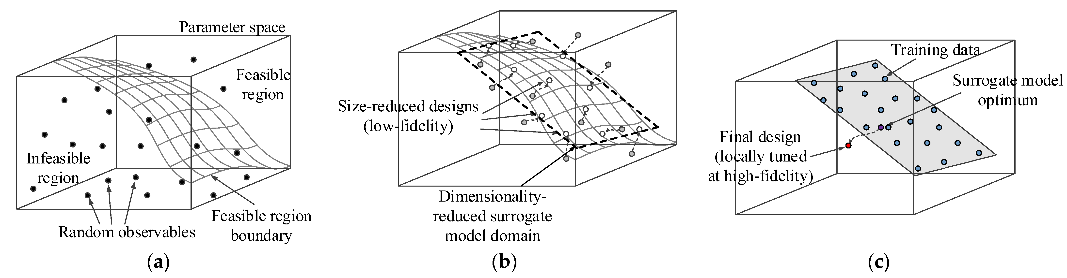
2.2. Globalized Size Reduction: The Concept

Compact antennas often exhibit parameter redundancy, being a result of introducing multitudinous topological modifications [21] and additional components into the basic radiators (e.g., monopoles [24]). As a result, there might be a number of combinations of designable parameters x that correspond to a relatively small antenna size and acceptable electrical performance. From the standpoint of numerical optimization, this is equivalent to the multimodality of size reduction task (2), i.e., the existence of multiple local optima. As explained in Section 1, the direct application of global search methods, in particular, population-based algorithms, is impractical due to the poor computational efficiency of such techniques. Similarly, the utilization of generic surrogate-assisted global optimizers (efficient global optimization, EGO [83,84]) is of limited use as a consequence of design space dimensionality and, to an even greater extent, because of broad parameter ranges. In this work, we propose an alternative approach that allows for at least partial mitigation of the mentioned difficulties, which includes globalized search and making the optimization outcome more immune to the supplied initial design.

The foundation of the proposed methodology is an exploration of the feasible region X_f boundary. The feasible region is a subset of the parameter space that comprises all vectors x satisfying the design constraints, i.e., such that g_k(x) ≤ 0, k = 1, …, n_g, and h_k(x) = 0, k = 1, …, n_h. Its boundary, X_b, is the set of vectors such that g_k(x) = 0 and h_k(x) = 0 for at least one of the constraints. As the reduction of antenna size deteriorates electrical and field performance figures, the minimum-size design has to be allocated on the boundary, i.e., at least one of the constraints is active. Consequently, it is beneficial to identify the spatial allocation of the boundary, X_b, and focus the search in the vicinity of this set. Figure 1 shows a visualization of the main concepts of the proposed optimization approach. The search process consists of several steps, which are presented in Figure 2. A detailed discussion of each stage will be provided in subsequent sections.

To enhance computational efficiency, the first three stages are carried out at the level of a low-fidelity (lower resolution) EM antenna model R_c. This is justified by the fact that at these stages, the evaluation accuracy is of minor importance. The reliability of the optimization process is secured by executing the final stages with the use of the high-fidelity EM model R_f. The remainder of this section contains a rigorous formulation for all stages as well as a summary of the complete workflow (Section 2.7).

2.3. Globalized Size Reduction: Approximating the Boundary of the Feasible Region

The design space of the antenna under study consists of an interval X = [lu]. We denote l and u as the lower and upper parameter bounds, respectively, i.e., the following holds l_k ≤ x_k ≤ u_k, k = 1, …, n. In the first stage of the optimization procedure, we generate N₁ random vectors x_r^(j) meeting the following requirements: (i) x_r^(j) ∈ [lu]; (ii) A₂ ≤ A(x_r^(j)) ≤ A₁; and (iii) the problem-dependent constraints are met at x_r^(j). Here, A₁ and A₂ represent the non-mandatory maximum and minimum antenna sizes, respectively, that might be known from the preceding work carried out on the same structure. It is also possible to introduce additional constraints that restrict the part of the design where sampling is to take place. The formulation of these constraints may involve the researcher’s know-how or other data garnered on the antenna at hand.

In the next step, we calculate low-fidelity antenna outputs, R_e(x_r⁽ⁱ⁾), j = 1, …, N₁, and designate a subset comprising N₂ entries {x_i^(j)}_j=1,…,N2 ⊂ {x_r^(j)}_j=1,…,Nl of vectors, which will serve as initial designs for miniaturization. This selection is carried out using an automated decision-making procedure, which takes into account respective constraint violation levels (with designs featuring violations of smaller magnitude being assessed as more beneficial). In the numerical experiments of Section 3, we set N₂ = 20, which is a good compromise between computational cost and the amount of information about the geometry of the boundary set X_b that may be attained with the selected designs. All points x_i^(j) are optimized for size reduction. In other words, for j = 1, …, N₂, starting from x⁽⁰⁾ = x_i^(j), we find

x_c^(j) = arg min{x : U(x)}

(3)

where U denotes the penalty-based merit function (2) and x_c^(j) are found with the use of the low-fidelity model R_c. Furthermore, task (3) is solved with relaxed convergence criteria to lower the computational expenditures associated with the optimization process: at this stage, the resolution of identifying the optimum design is not of major concern. Problem (3) is solved using a trust-region (TR), gradient-based algorithm [86]. The details of the TR algorithm will be given in Section 2.6.

In the last step of this stage, an N₃-element of {x_c^(j)}_j=1,…,N2 has to be selected, such that it encompasses the vectors of satisfactory quality with regard to constraint violation. This eliminates vectors at which optimization process (3) failed for any reason. For example, a typical selection criterion for impedance matching constraints would be to eliminate designs for which constraint violation at x_c^(j) exceeds 2 dB. In the next section, we will refer to the selected subset simply as {x_c^(j)}_j=1,…,N3.

2.4. Globalized Size Reduction: Constructing a Surrogate Model

The designs {x_c^(j)}_j=1,…,N3 provide an approximate allocation of a part of the feasible region boundary. These vectors will be used to establish a metamodel domain to be assessed for the purpose of globalized optimization of antenna size. In order to facilitate and lower the surrogate model setup cost, the domain will be of reduced dimensionality using the procedure proposed in [43], which is explained in Figure 3.

In our approach, we assume that N₃ > n (dimensionality of the design space; see also Figure 3). The model domain X_p refers to the set encompassing every design x_c^(j), j = 1, …, N₃ alongside the selected p directions. In most cases, the correlation between designs x_c^(j) is rather strong, which means that restricting the domain to the first few dominant eigenvectors is sufficient. Dimensionality reduction allows for rendering reliable models with the use of relatively small training datasets. In our experiments in Section 3, we use p = 3 for all verification cases.

The surrogate model itself is set up as a kriging interpolation model [87]. The training set x_B^(j) ∈ X_p, j = 1, …, N₄ is allocated with the use of Latin hypercube sampling (LHS) [88]. In Section 3, we use N₄ = 200 high-fidelity training data samples, which allows us to maintain the relative RMS error in the metamodel of around a few percent.

However, the alignment of the domain with the coordinate system axes is not preserved; therefore, the design of the experiment technique has to be slightly more involved. More specifically, the dataset is first allocated using LHS in the unity interval 0 ≤ z_j ≤ 1, j = 1, …, k. Subsequently, the normalized data points z = [z₁ … z_n]^T are mapped into the domain X_p as $y=h(z)=x_c+{\displaystyle \sum _{k=1}^p(2z_k-1){\lambda }_{b_k}{a}_k}$.

2.5. Globalized Size Reduction: Surrogate Optimization

Global optimization of the surrogate model within its domain X_p is arranged as a two-stage process. In the first step, a search grid M_p is prepared, which consists of all vectors in the form

$$M_p=\left\{\begin{array}{c}x=x_c+{\displaystyle {\sum }_{k=1}^p(2{\lambda }_k-1){\lambda }_{b_k}{a}_k}\\ {\lambda }_k\in \left\{0,1/K,2/K,\dots ,1\right\},\hspace{0.17em}\hspace{0.17em}k=1,\dots ,p\end{array}\right\}$$

(4)

where K stands for the grid density. In our numerical experiments, we set K = 20. The starting point x_g⁽⁰⁾ is assessed as

$$x_g^{(0)}=\arg \underset{}{\min }\left\{x\in M_p\cap X:U(x)\right\}$$

(5)

In other words, the design x_g⁽⁰⁾ minimizes the objective function U (evaluated using the surrogate model) over the intersection of the design space X and search grid.

The second stage is local surrogate-based miniaturization within X_p ∩ X, as in (2). The task is solved using the trust-region gradient search (Section 2.6). The design found this way is denoted as x_g⁽⁰⁾.

2.6. Globalized Size Reduction: Final Tuning

The last step of the proposed globalized optimization procedure is a local tuning of antenna parameters for a minimum size, performed with the high-fidelity model R_f. The underlying optimization algorithm is the trust-region (TR) gradient search [86], as briefly outlined in this section. As mentioned before, the same algorithm is used to perform low-fidelity optimization runs (3) in Section 2.3, as well as to refine the surrogate model in Section 2.5.

The trust-region procedure renders a series of approximate solutions x⁽ⁱ⁾, i = 0, 1, … to the optimal design x^* of (2). The starting point is the design x_g⁽⁰⁾, found as delineated in Section 2.5. We have

$$x^{(i+1)}=\arg \underset{\left|\right|x-x^{(i)}\left|\right|\le d^{(i)}}{\min }{U}_L^{(i)}(x)$$

(6)

where U_L⁽ⁱ⁾ is a merit function evaluated as in (3) but using the first-order Taylor expansion model for antenna responses, L⁽ⁱ⁾, evaluated at the current design x⁽ⁱ⁾. The model is defined as

$$L_{}^{(i)}(x)=R_f(x^{(i)})+J_f(x^{(i)})\cdot (x-x^{(i)})$$

(7)

In (7), the Jacobian matrix of the high-fidelity response R_f at x⁽ⁱ⁾ is referred to as J(x⁽ⁱ⁾), calculated using finite differentiation. The search radius d⁽ⁱ⁾ is adaptively modified using the standard TR setup [86]. If U(x⁽ⁱ⁺¹⁾) < U(x⁽ⁱ⁾), the solution x⁽ⁱ⁺¹⁾ produced by (6) is accepted; otherwise, the size parameter d⁽ⁱ⁾ is set to a smaller value, and the iteration is repeated. The algorithm is terminated if ||x⁽ⁱ⁺¹⁾ − x⁽ⁱ⁾|| < ε (convergence in argument) or d⁽ⁱ⁾ < ε. In the final refinement of the high-fidelity model, the termination threshold of 10⁻³ is used, whereas for low-fidelity miniaturization (cf. (3)), it is increased to 10⁻².

2.7. Globalized Size Reduction: Complete Algorithm

In this section, we summarize the operation of the entire globalized size reduction procedure. The major control parameters are gathered in

Table 2. Globalized size reduction procedure: control parameters.

Parameter	Description and Recommendations
Nr	Cardinality of the observable set
	Recommended value: from 50 to 100; the higher the design space dimensionality n, the larger Nr should be used
p	Dimensionality of the surrogate domain
	Recommended value: p = 3 (in order to ensure good model scalability as a function of the number of training samples; should take into account the eigenvalues λk)
NB	Cardinality of the training data set (for surrogate model construction)
	Recommended values to ensure a relative RMS error of a few percent: from 200 to 500

. These parameters were already commented upon in Section 2.2, Section 2.3, Section 2.4 and Section 2.5. The values shown in the table are used for all verification cases presented in Section 3.

3. Validation

This section provides a validation of the proposed globalized miniaturization algorithm presented in Section 2 using four examples of broadband microstrip antennas. For each structure, an optimization for minimum size is carried out with a constraint imposed on their reflection levels. The performance of the proposed procedure is compared to a multi-start local search involving implicit constraint handling and both fixed and adaptive penalty coefficients, along with a popular nature-inspired particle swarm optimizer (PSO) (global optimizer). Section 3.1 outlines the verification antenna structures and describes the setup of numerical experiments as well as briefly characterizes the benchmark algorithms. A presentation and discussion of the results are provided in Section 3.2 and Section 3.3, respectively.

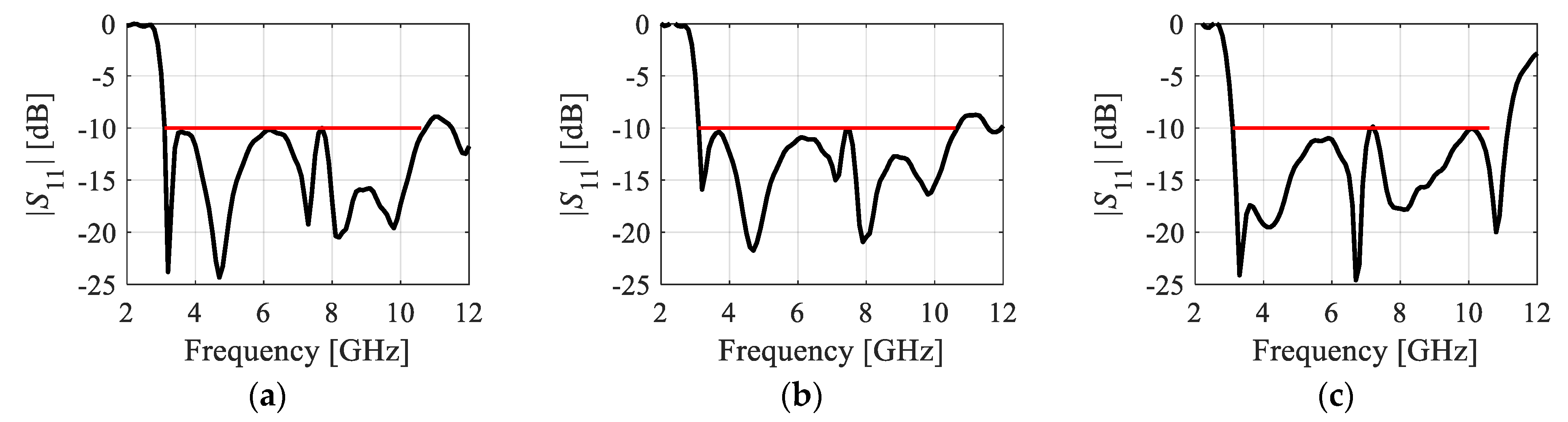
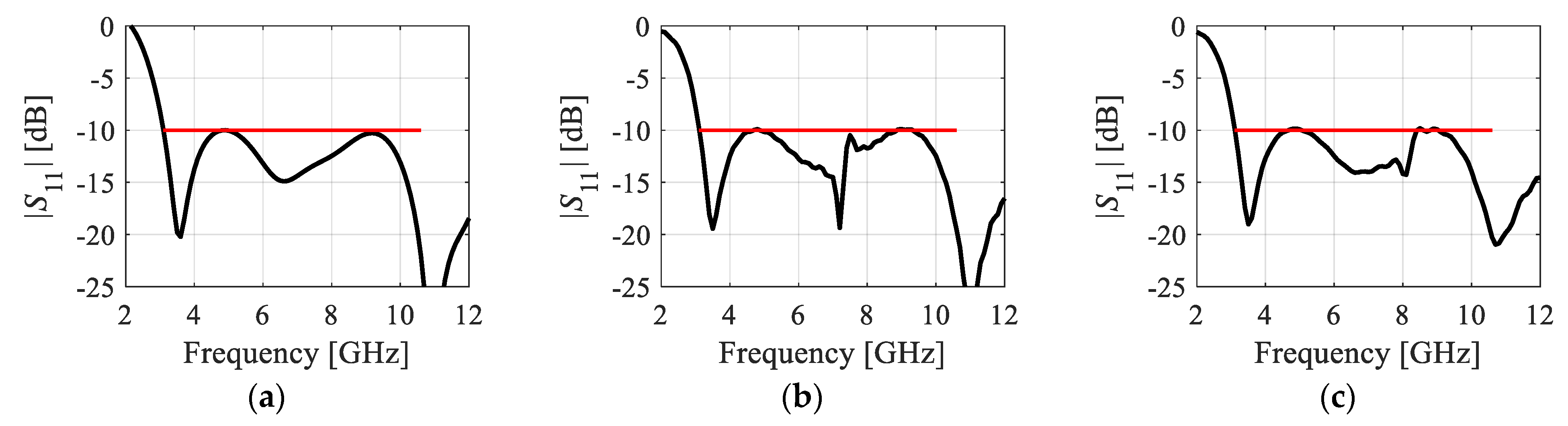
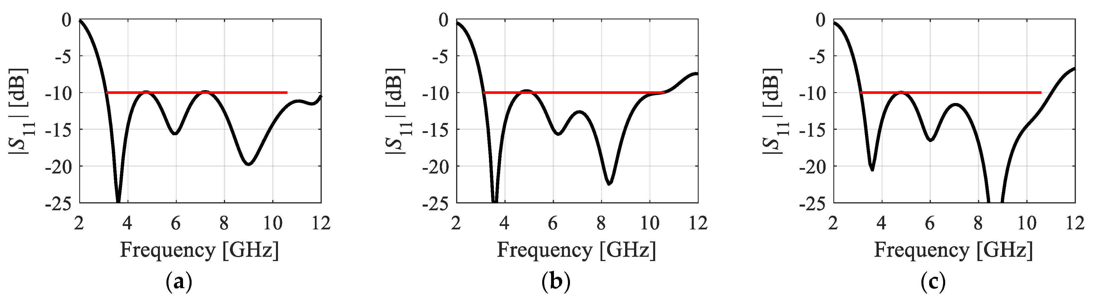
3.1. Antenna Structures and Numerical Experiment Setup

The proposed algorithm is validated with the use of four broadband microstrip antenna structures, as presented in Figure 4.

Table 3. Antenna structures used to validate the proposed algorithm.

Antenna	I [89]	II [90]	III [91]	IV [92]
Substrate	RF-35	RF-35	FR-4	RO4350
	(εr = 3.5, h = 0.762 mm)	(εr = 3.5, h = 0.762 mm)	(εr = 4.4, h = 1.52 mm)	(εr = 3.48, h = 0.762 mm)
Designable Parameters (mm)	x = [l0 g a l1 l2 w1 o]T	x = [L0 dR R rrel dL dw Lg L1 R1 dr crel]T	x = [L0 dR R rrel dL dw Lg L1 R1 dr crel]T	x = [L0 L1 L2 L dL Lg w1 w2 w dw Ls ws c]T
Other Parameters (mm)	w0 = 2o + a, wf = 1.7	w0 = 1.7	W0 = 3.0	w0 = 1.7
Parameter space X	l = [10 8 4 5 1 0.1 0.2]T	l = [4 0 3 0.1 0 0 4 0 2 0.2 0.2]T	l = [2 2 2 0.2 2 0 0.1 0.1 0 0.01 0.01]T	l = [5 0.1 0.1 5 0 5 0.1 0.1 5 0 0.01 0.1 0.01]T
	u = [35 20 15 12 15 10 3]T	u = [15 6 8 0.9 5 8 15 6 5 1 0.9]T	u = [15 15 20 3 15 15 3 8 5 0.8 0.8]T	u = [20 2 3 20 5 20 1 1 25 10 0.2 0.9 0.3]T
Intended operating band	Ultra-wideband frequency band from 3.1 GHz to 10.6 GHz
Design objective *	Reduce antenna size A(x) (understood as the substrate footprint area containing the device)
EM model	Evaluated using time-domain solver in CST Microwave Studio (models incorporate SMA connectors)
High-fidelity EM model	~900,000 mesh cells	~2,300,000 mesh cells	~1,080,000 mesh cells	~470,000 mesh cells
	Simulation time 150 s	Simulation time 424 s	Simulation time 265 s	Simulation time 105 s
Low-fidelity EM model	~130,000 mesh cells	~210,000 mesh cells	~160,000 mesh cells	~130,000 mesh cells
	Simulation time 45 s	Simulation time 51 s	Simulation time 55 s	Simulation time 37 s

* The size reduction problem is subject to a constraint: |S₁₁(x,f)| ≤ −10 dB for f ∈ [3.1 10.6] GHz, which is handled using the penalty function shown in the second row of Table 1, with the penalty coefficient β = 10⁴.

provides additional information concerning the antennas (see also [89,90,91,92]). All the simulations have been performed using Intel Xeon 2.1 GHz dual-core CPU with 128 GB RAM. The low-fidelity models constitute coarse-discretization versions of the high-fidelity representations. The last two rows of Table 3 provide information about the simulation times for the respective models. As the average time evaluation ratio between the high- and low-fidelity models is over four, considerable time savings while executing the first few stages of the proposed algorithm are obtained. The proposed algorithm is compared to several benchmark methods, which are characterized in

Table 4. Benchmark procedures.

Algorithm	Operating Principles
I	Local gradient-based miniaturization with the trust region algorithm used as a search engine (cf. Section 2.6). The size reduction task is expressed as (2) and (3). The penalty coefficient β is kept fixed throughout the algorithm run.
	Algorithm performance highly depends on the choice of β: small values ensure better miniaturization rates but lead to larger constraint violations; a large β leads to a more precise constraint control but inferior size reduction because of the objective function (2) steepness near the feasible region boundary.
	The algorithm is executed for different values of β = 103, 104, and 105.
II	Local trust-region search with adaptively adjusted penalty coefficients [89]. This method adjusts the value of β during the algorithm run based on the constraint violation detected in the current iteration. This leads to a better overall performance with regard to size reduction and constraint control [89].
III	The particle swarm optimizer (PSO) [93] is a widely used population-based algorithm. The following PSO setup is used: the swarm size is set to 10, the maximal number of iterations is 100, and the typical control parameters are (χ = 0.73, c1 = c2 = 2.05), cf. [89]. The penalty coefficient of problem (2) is set to 104.
	Note that the PSO is set up here with a relatively small computational budget (1000 objective function evaluations) in order to avoid excessive computational costs, which are still in the range of a few days of the CPU time per algorithm run.

.

All the considered EM-driven miniaturization tasks are multimodal due to a variety of geometrical modifications used in the considered structures (e.g., L-shaped stub in Antennas I and II, radiator slots in Antennas II, III, and IV, and a ground-plane slit in Antenna III). Thus, the results obtained using the local search might be highly dependent on the initial design. Moreover, when using globalized methods, the results will also differ between the algorithm runs because of design space dimensionality and its large volume resulting from broad ranges for most of geometry parameters. Thus, we verify the algorithm performance in a statistical manner: based on ten independent runs of all methods. We compare the average antenna size and its standard deviation, the average constraint violation and its standard deviation, along with the average optimization computational cost.

3.2. Results

Table 5. Optimization results for Antenna I.

Optimization Algorithm		Performance Figure
		Antenna Footprint A (mm2) 1	Std(A) 2	Constraint Violation D (dB) 3	Std(D) (dB) 4	CPU Cost 5
Algorithm I	β = 103	318.1	42.6	1.2	0.4	43.8 × Rf (1.8 h)
	β = 104	317.7	42.3	0.4	0.7	42.2 × Rf (1.8 h)
	β = 105	318.8	43.3	0.1	0.2	41.4 × Rf (1.7 h)
Algorithm II		314.1	42.3	0.3	0.2	50.0 × Rf (2.1 h)
Algorithm III		360.9	67.5	0.5	0.9	1000 × Rf (42 h)
Globalized search with dimensionality reduction (this work)		265.4	9.6	0.1	0.1	692.7 × Rf (29 h)

¹ Optimized antenna footprint A averaged over ten algorithm runs. ² Std(A)—standard deviation of the optimized antenna footprint averaged over ten algorithm runs. ³ Constraint violation, defined as D = {3.1 GHz ≤ f ≤ 10.6 GHz : max|S₁₁(f)|} + 10, averaged over ten algorithm runs; |S₁₁(f)|—antenna reflection. ⁴ Std(D)—standard deviation of the constraint violation D, averaged over ten algorithm runs. ⁵ Cost expressed in terms of the equivalent number of high-fidelity EM antenna analyses. Numbers in brackets correspond to the running time in hours.

,

Table 6. Optimization results for Antenna II.

Optimization Algorithm		Performance Figure
		Antenna Footprint A (mm2) 1	Std(A) 2	Constraint Violation D (dB) 3	Std(D) (dB) 4	CPU Cost 5
Algorithm I	β = 103	250.4	24.0	1.2	0.5	124.2 × Rf (14.6 h)
	β = 104	318.6	60.0	0.1	0.1	180.3 × Rf (21.2 h)
	β = 105	331.6	63.4	0.1	0.1	133.2 × Rf (15.7 h)
Algorithm II		281.6	37.1	0.2	0.2	181.7 × Rf (21.4 h)
Algorithm III		399.4	143.6	0.6	0.4	1000 × Rf (118 h)
Globalized search with dimensionality reduction (this work)		205.6	18.2	0.07	0.07	472.6 × Rf (56 h)

¹ Optimized antenna footprint A averaged over ten algorithm runs. ² Std(A)—standard deviation of the optimized antenna footprint averaged over ten algorithm runs. ³ Constraint violation, defined as D = {3.1 GHz ≤ f ≤ 10.6 GHz : max|S₁₁(f)|} + 10, averaged over ten algorithm runs; |S₁₁(f)|—antenna reflection. ⁴ Std(D)—standard deviation of the constraint violation D, averaged over ten algorithm runs. ⁵ Cost expressed in terms of the equivalent number of high-fidelity EM antenna analyses. Numbers in brackets correspond to the running time in hours.

,

Table 7. Optimization results for Antenna III.

Optimization Algorithm		Performance Figure
		Antenna Footprint A (mm2) 1	Std(A) 2	Constraint Violation D (dB) 3	Std(D) (dB) 4	CPU Cost 5
Algorithm I	β = 103	212.8	14.3	1.0	0.4	164.9 × Rf (12.1 h)
	β = 104	255.0	25.1	0.2	0.1	138.1 × Rf (10.2 h)
	β = 105	280.1	47.4	0.1	0.1	154.0 × Rf (11.3 h)
Algorithm II		215.6	3.6	0.3	0.1	189.9 × Rf (14.0 h)
Algorithm III		425.7	145.8	0.2	0.2	1000 × Rf (74 h)
Globalized search with dimensionality reduction (this work)		226.2	12.4	0.1	0.1	689.7 × Rf (51 h)

¹ Optimized antenna footprint A averaged over ten algorithm runs. ² Std(A)—standard deviation of the optimized antenna footprint averaged over ten algorithm runs. ³ Constraint violation, defined as D = {3.1 GHz ≤ f ≤ 10.6 GHz : max|S₁₁(f)|} + 10, averaged over ten algorithm runs; |S₁₁(f)|—antenna reflection. ⁴ Std(D)—standard deviation of the constraint violation D, averaged over ten algorithm runs. ⁵ Cost expressed in terms of the equivalent number of high-fidelity EM antenna analyses. Numbers in brackets correspond to the running time in hours.

and

Table 8. Optimization results for Antenna IV.

Optimization Algorithm		Performance Figure
		Antenna Footprint A (mm2) 1	Std(A) 2	Constraint Violation D (dB) 3	Std(D) (dB) 4	CPU Cost 5
Algorithm I	β = 103	727.9	236.0	1.7	1.5	180.3 × Rf (5.3 h)
	β = 104	829.5	206.4	1.0	1.9	211.2 × Rf (6.2 h)
	β = 105	842.8	130.2	0.4	0.9	248.0 × Rf (7.2 h)
Algorithm II		753.9	243.0	0.9	0.8	230.3 × Rf (6.7 h)
Algorithm III		457.8	59.1	0.7	0.4	1000 × Rf (29 h)
Globalized search with dimensionality reduction (this work)		414.8	10.4	0.3	0.1	922.5 × Rf (26.9 h)

¹ Optimized antenna footprint A averaged over ten algorithm runs. ² Std(A)—standard deviation of the optimized antenna footprint averaged over ten algorithm runs. ³ Constraint violation, defined as D = {3.1 GHz ≤ f ≤ 10.6 GHz : max|S₁₁(f)|} + 10, averaged over ten algorithm runs; |S₁₁(f)|—antenna reflection. ⁴ Std(D)—standard deviation of the constraint violation D, averaged over ten algorithm runs. ⁵ Cost expressed in terms of the equivalent number of high-fidelity EM antenna analyses. Numbers in brackets correspond to the running time in hours.

present the results achieved using the presented procedure and the benchmark routines. Figure 5, Figure 6, Figure 7 and Figure 8 illustrate the reflection characteristics of the antennas optimized using our technique for three selected algorithm runs for each structure. The numerical data includes the average footprint area and its standard deviation, the average constraint violation and its standard deviation, and the average optimization cost. The standard deviations can be viewed as a measure of result repeatability. The results are discussed at length in Section 3.3. The experimental validation of the antenna structures themselves can be found in the source papers (e.g., [89,90,91,92]). It is not included here as it is irrelevant to the main topic of the work.

3.3. Result Analysis

The results presented in Table 5, Table 6, Table 7 and Table 8 permit us to summarize the performance of the introduced globalized size reduction algorithm and how it compares to the benchmark methods.

The obtained results confirm that the considered miniaturization tasks are indeed multimodal, which is implied by the high standard deviation values of the antenna size A for Algorithms I and II, which are both local methods. In particular, depending on the initial design, the obtained footprint area may vary significantly and by as much as thirty percent with respect to the average size.

A comparison of the proposed procedure with the benchmark algorithms allows us to draw the following conclusions. As expected, and already demonstrated in the literature (e.g., [89]), the outcome of Algorithm I depends on the penalty coefficient setup. When using low values of β, excessive constraint violations occur, whereas using coefficients that are too high leads to inferior miniaturization rates. Algorithm II resolves these issues to a certain extent by ensuring both the constraint control and competitive (w.r.t. Algorithm I) antenna sizes. The computational cost of Algorithm II is only slightly higher than that of Algorithm I.

As far as the nature-inspired optimization (Algorithm III) is concerned, it performs poorly for all considered antenna structures, both with regard to the achieved antenna footprint areas and constraint violations. The reasons are twofold: (i) the intrinsic challenges of the size reduction task and (ii) the low computational budget assigned for the algorithm. As explained before, we use this setup to avoid excessive computational costs. The most important takeaway here is that 1000 EM analyses are—to a large extent—insufficient to yield satisfactory optimization outcomes using population-based techniques.

Overall, the size reduction procedure proposed in this work is demonstrated to outperform all benchmark algorithms in terms of size reduction. On the one hand, it yields designs featuring considerably smaller average footprint area (e.g., the improvement over Algorithm II is almost thirty percent) except for Antenna III, where the obtained average size is comparable to Algorithm II. Yet, the standard deviation of the antenna size is significantly lower for most of the considered structures (by almost 80% for Antenna I, over 50% for Antenna II, and over 95% for Antenna IV; all with respect to Algorithm II) and comparable for Antenna III. The latter corroborates the global search capability of the presented approach.

In terms of computational cost, the proposed method is clearly more expensive than local routines, although the difference is not significant for Antennas II and III. Still, the overall expenses equal to a few hundred EM simulations is very much practical given the huge advantages in terms of the optimization process reliability ensured with our technique. Also, the comparison to PSO, executed with a computational budget of 1000 EM simulations (i.e., almost twice as high as the typical cost of the proposed method), provides important indications concerning the performance of nature-inspired procedures for the considered class of size reduction tasks. Based on a typical evolution of the objective function value for population-based methods (rapid initial decrease followed by a plateau), it is expected that reaching the design quality offered by the proposed method would require many thousand EM analyses, if possible at all.

Furthermore, one can observe that Antenna IV is by far the most challenging case, primarily due to the number of its geometry parameters (thirteen). All benchmark algorithms, including Algorithm II (adaptive penalty factors), perform poorly for this structure, not only in terms of achievable miniaturization rates and solution repeatability but also in constraint control. At the same time, Algorithm III (PSO) performs considerably better than both Algorithms I and II, which confirms the challenging nature of this case study. Notwithstanding, the proposed procedure produces results that are superior to all benchmark methods. It yields designs with average antenna sizes being about half of that obtained using Algorithms I and II, a standard deviation almost six times smaller than Algorithm III, and excellent enforcement of the design constraint.

The collective performance of the introduced globalized size reduction approach is encouraging, both in terms of the average size reduction ratio, the solution repeatability, and computational efficacy. The latter means that although the CPU expenses of our procedure are higher than those of local algorithms (Algorithms I and II), the difference is not overwhelming given the efficacy benefits. The reliability of the developed globalized knowledge-based miniaturization framework results from an accurate identification of the feasible region boundary, where the designs meeting the size-reduction-related design specifications reside. This identification is carried out by extracting knowledge on actual constraint violations from random observables as well as the use of an automated decision-making procedure, which selects observables of sufficient quality. At the same time, the costs are practically acceptable and significantly lower than what is required using nature-inspired methods. This is possible due to the use of variable-fidelity EM simulations as well as dimensionality reduction when defining the domain of the surrogate. Note that both mechanisms compromise accuracy; notwithstanding, this does not affect overall reliability because all simplifications are pertinent to the intermediate stages of the optimization process. The final steps, i.e., the construction of the surrogate model and the final tuning, are both executed at the high-fidelity level.

4. Conclusions

This work introduced a novel framework for EM-based size reduction of antenna structures. Our methodology enables global search with an initial knowledge-based pre-screening of the design space and approximating the geometry of the feasible region boundary using supplementary optimization processes, both executed at the low-fidelity (thus computationally cheaper) level of evaluating antenna responses. Furthermore, it allows for exploring the boundary region using dimensionality-reduced surrogate modeling methods. The reliability of the procedure is secured by executing the last stages (surrogate model identification and final parameter tuning) at the high-fidelity EM simulation level. The presented technique is comprehensively validated using four microstrip antenna structures and benchmarked against several algorithms, including both local (gradient-based) routines and a representative nature-inspired algorithm (PSO). The results corroborate the globalized search capability of the proposed procedure and its superior overall performance. On the one hand, it consistently ensures improved miniaturization rates over the benchmark. The obtained designs are up to fifty percent smaller with a twenty-five percent average. Further, it provides good repeatability of solutions, as indicated by low standard deviations of the antenna sizes, which are from six to as much as twenty-four times smaller than for the benchmark procedures, with an average of twelve. On the other hand, owing to the implemented mechanisms, especially variable-resolution models and dimensionality reduction, the proposed approach retains relatively low computational cost. The savings with respect to the PSO algorithm are about thirty percent, with the latter yielding designs of considerably larger footprints, even twice as larger. Our future work will be aimed at further development of this methodology, especially in terms of ensuring a more extensive exploration of the feasible region boundary, as well as applying it to the various classes of antenna and microwave components.

References

1. Ameen, M.; Thummaluru, S.R.; Chaudhary, R.K. A compact multilayer triple-band circularly polarized antenna using anisotropic polarization converter. IEEE Antennas Wirel. Propag. Lett. 2021, 20, 145–149. [Google Scholar] [CrossRef]
2. Cheng, T.; Jiang, W.; Gong, S.; Yu, Y. Broadband SIW cavity-backed modified dumbbell-shaped slot antenna. IEEE Antennas Wirel. Propag. Lett. 2019, 18, 936–940. [Google Scholar] [CrossRef]
3. Huang, H.; Gao, S.; Lin, S.; Ge, L. A wideband water patch antenna with polarization diversity. IEEE Antennas Wirel. Propag. Lett. 2020, 19, 1113–1117. [Google Scholar] [CrossRef]
4. Ullah, U.; Al-Hasan, M.; Koziel, S.; Ben Mabrouk, I. Series-slot-fed circularly polarized multiple-input-multiple-output antenna array enabling circular polarization diversity for 5G 28-GHz indoor applications. IEEE Trans. Antennas Propag. 2021, 69, 5607–5616. [Google Scholar] [CrossRef]
5. Ali, M.Z.; Khan, Q.U. High gain backward scanning substrate integrated waveguide leaky wave antenna. IEEE Trans. Antennas Propag. 2021, 69, 562–565. [Google Scholar] [CrossRef]
6. Chopra, R.; Kumar, G. Series-fed binomial microstrip arrays for extremely low sidelobe level. IEEE Trans. Antennas Propag. 2019, 67, 4275–4279. [Google Scholar] [CrossRef]
7. Karmokar, D.K.; Esselle, K.P.; Bird, T.S. Wideband microstrip leaky-wave antennas with two symmetrical side beams for simultaneous dual-beam scanning. IEEE Trans. Antennas Propag. 2016, 64, 1262–1269. [Google Scholar] [CrossRef]
8. Shirazi, M.; Li, T.; Huang, J.; Gong, X. A reconfigurable dual-polarization slot-ring antenna element with wide bandwidth for array applications. IEEE Trans. Antennas Propag. 2018, 66, 5943–5954. [Google Scholar] [CrossRef]
9. Yang, Z.; Browning, K.C.; Warnick, K.F. High-efficiency stacked shorted annular patch antenna feed for Ku-Band satellite communications. IEEE Trans. Antennas Propag. 2016, 64, 2568–2572. [Google Scholar] [CrossRef]
10. Oh, J.I.; Jo, H.W.; Kim, K.S.; Cho, H.; Yu, J.W. A compact cavity-backed slot antenna using dual mode for IoT applications. IEEE Antennas Wirel. Propag. Lett. 2021, 20, 317–321. [Google Scholar] [CrossRef]
11. Santamaria, L.; Ferrero, F.; Staraj, R.; Lizzi, L. Electronically pattern reconfigurable antenna for IoT applications. IEEE Open J. Antennas Propag. 2021, 2, 546–554. [Google Scholar] [CrossRef]
12. Mahmud, M.Z.; Islam, M.T.; Misran, N.; Kibria, S.; Samsuzzaman, M. Microwave imaging for breast tumor detection using uniplanar AMC based CPW-fed microstrip antenna. IEEE Access 2018, 6, 44763–44775. [Google Scholar] [CrossRef]
13. Sun, L.; Li, Y.; Zhang, Z. Wideband decoupling of integrated slot antenna pairs for 5G smartphones. IEEE Trans. Antennas Propag. 2021, 69, 2386–2391. [Google Scholar] [CrossRef]
14. Chen, X.; Yang, L.; Zhao, J.; Fu, G. High-efficiency compact circularly polarized microstrip antenna with wide beamwidth for airborne communication. IEEE Antennas Wirel. Propag. Lett. 2016, 15, 1518–1521. [Google Scholar] [CrossRef]
15. Yoo, S.; Milyakh, Y.; Kim, H.; Hong, C.; Choo, H. Patch array antenna using a dual coupled feeding structure for 79 GHz automotive radar applications. IEEE Antennas Wirel. Propag. Lett. 2020, 19, 676–679. [Google Scholar] [CrossRef]
16. Xu, L.; Xu, J.; Chu, Z.; Liu, S.; Zhu, X. Circularly polarized implantable antenna with improved impedance matching. IEEE Antennas Wirel. Propag. Lett. 2020, 19, 876–880. [Google Scholar] [CrossRef]
17. Koziel, S.; Cheng, Q.S.; Li, S. Optimization-driven antenna design framework with multiple performance constraints. Int. J. RF Microw. Comput. Aided Eng. 2018, 28, e21208. [Google Scholar] [CrossRef]
18. Liu, J.; Esselle, K.P.; Hay, S.G.; Zhong, S. Effects of printed UWB antenna miniaturization on pulse fidelity and pattern stability. IEEE Trans. Antennas Propag. 2014, 62, 3903–3910. [Google Scholar] [CrossRef]
19. Roshna, T.K.; Deepak, U.; Sajitha, V.R.; Vasudevan, K.; Mohanan, P. A compact UWB MIMO antenna with reflector to enhance isolation. IEEE Trans. Antennas Propag. 2015, 63, 1873–1877. [Google Scholar] [CrossRef]
20. Wen, L.; Gao, S.; Luo, Q.; Yang, Q.; Hu, W.; Yin, Y.; Wu, J.; Ren, X. A wideband series-fed circularly polarized differential antenna by using crossed open slot-pairs. IEEE Trans. Antennas Propag. 2020, 68, 2565–2574. [Google Scholar] [CrossRef] [Green Version]
21. Roshani, S.; Roshani, S. A compact coupler design using meandered line compact microstrip resonant cell (MLCMRC) and bended lines. Wirel. Netw. 2021, 27, 677–684. [Google Scholar] [CrossRef]
22. Reddy, V.V.; Sarma, N.V.S.N. Compact circularly polarized asymmetrical fractal boundary microstrip antenna for wireless applications. IEEE Antennas Wireless Propag. Lett. 2014, 13, 118–121. [Google Scholar] [CrossRef]
23. Haq, M.A.; Koziel, S. Feed line alterations for optimization-based design of compact super wideband MIMO antennas in parallel configuration. IEEE Antennas Wireless Propag. Lett. 2019, 18, 1986–1990. [Google Scholar]
24. Haq, M.A.; Koziel, S. Ground plane alterations for design of high-isolation compact wideband MIMO antenna. IEEE Access 2018, 6, 48978–48983. [Google Scholar] [CrossRef]
25. Hu, W.; Yin, Y.; Yang, X.; Fei, P. Compact multiresonator-loaded planar antenna for multiband operation. IEEE Trans. Antennas Propag. 2013, 61, 2838–2841. [Google Scholar] [CrossRef]
26. Podilchak, S.K.; Johnstone, J.C.; Caillet, M.; Clénet, M.; Antar, Y.M.M. A compact wideband dielectric resonator antenna with a meandered slot ring and cavity backing. IEEE Antennas Wirel. Propag. Lett. 2016, 15, 909–913. [Google Scholar] [CrossRef]
27. Ding, K.; Gao, C.; Qu, D.; Yin, Q. Compact broadband MIMO antenna with parasitic strip. IEEE Antennas Wirel. Propag. Lett. 2017, 16, 2349–2353. [Google Scholar] [CrossRef]
28. Teni, G.; Zhang, N.; Qiu, J.; Zhang, P. Research on a novel miniaturized antipodal Vivaldi antenna with improved radiation. IEEE Antennas Wirel. Propag. Lett. 2013, 12, 417–420. [Google Scholar] [CrossRef]
29. Qin, X.; Li, Y. Compact dual-polarized cross-slot antenna with colocated feeding. IEEE Trans. Antennas Propag. 2019, 67, 7139–7143. [Google Scholar] [CrossRef]
30. Tu, W.H.; Hsu, S.H.; Chang, K. Compact 5.8-GHz rectenna using stepped-impedance dipole antenna. IEEE Antennas Wirel. Propag. Lett. 2007, 6, 282–284. [Google Scholar] [CrossRef]
31. Ding, Z.; Jin, R.; Geng, J.; Zhu, W.; Liang, X. Varactor loaded pattern reconfigurable patch antenna with shorting pins. IEEE Trans. Antennas Propag. 2019, 67, 6267–6277. [Google Scholar] [CrossRef]
32. Park, J.P.; Han, S.M.; Itoh, T. A rectenna design with harmonic-rejecting circular-sector antenna. IEEE Antennas Wirel. Propag. Lett. 2004, 3, 52–54. [Google Scholar] [CrossRef]
33. Prajapati, P.R.; Murthy, G.G.K.; Patnaik, A.; Kartikeyan, M.V. Design and testing of a compact circularly polarised microstrip antenna with fractal defected ground structure for L-band applications. IET Microw. Antennas Propag. 2015, 9, 1179–1185. [Google Scholar] [CrossRef]
34. Haq, M.A.; Koziel, S. Simulation-based optimization for rigorous assessment of ground plane modifications in compact UWB antenna design. Int. J. RF Microw. CAE 2018, 28, e21204. [Google Scholar] [CrossRef]
35. Yousif, S.; Saka, M.P. Optimum design of post-tensioned flat slabs with its columns to ACI 318-11 using population based beetle antenna search algorithm. Comput. Struct. 2021, 256, 106520. [Google Scholar] [CrossRef]
36. Kovaleva, M.; Bulger, D.; Esselle, K.P. Comparative study of optimization algorithms on the design of broadband antennas. IEEE J. Multiscale Multiphys. Comput. Tech. 2020, 5, 89–98. [Google Scholar] [CrossRef]
37. Koziel, S.; Pietrenko-Dabrowska, A.; Al-Hasan, M. Frequency-based regularization for improved reliability optimization of antenna structures. IEEE Trans. Antennas Propag. 2020, 69, 4246–4251. [Google Scholar] [CrossRef]
38. Sang, L.; Wu, S.; Liu, G.; Wang, J.; Huang, W. High-gain UWB Vivaldi antenna loaded with reconfigurable 3-D phase adjusting unit lens. IEEE Antennas Wirel. Propag. Lett. 2020, 19, 322–326. [Google Scholar] [CrossRef]
39. Bianchi, D.; Genovesi, S.; Monorchio, A. Fast optimization of ultra-broadband antennas with distributed matching networks. IEEE Antennas Wirel. Propag. Lett. 2014, 13, 642–645. [Google Scholar] [CrossRef]
40. Liu, Y.; Li, M.; Haupt, R.L.; Guo, Y.J. Synthesizing shaped power patterns for linear and planar antenna arrays including mutual coupling by refined joint rotation/phase optimization. IEEE Trans. Antennas Propag. 2020, 68, 4648–4657. [Google Scholar] [CrossRef]
41. Niu, Z.; Zhang, H.; Chen, Q.; Zhong, T. Isolation enhancement in closely coupled dual-band MIMO patch antennas. IEEE Antennas Wirel. Propag. Lett. 2019, 18, 1686–1690. [Google Scholar] [CrossRef]
42. Du, J.; Roblin, C. Statistical modeling of disturbed antennas based on the polynomial chaos expansion. IEEE Antennas Wirel. Propag. Lett. 2017, 16, 1843–1847. [Google Scholar] [CrossRef]
43. Koziel, S.; Pietrenko-Dabrowska, A. Fast multi-objective optimization of antenna structures by means of data-driven surrogates and dimensionality reduction. IEEE Access 2020, 8, 183300–183311. [Google Scholar] [CrossRef]
44. Laware, A.R.; Navthar, R.R.; Bandal, V.S.; Talange, D.B. Global optimization of second-order sliding mode controller parameters using a new sliding surface: An experimental verification to process control system. ISA Trans. 2022, 126, 498–512. [Google Scholar] [CrossRef]
45. Ren, Z.; He, S.; Zhang, D.; Zhang, Y.; Koh, C.S. A possibility-based robust optimal design algorithm in preliminary design state of electromagnetic devices. IEEE Trans. Magn. 2016, 52, 7001504. [Google Scholar] [CrossRef]
46. Hassan, E.; Noreland, D.; Augustine, R.; Wadbro, E.; Berggren, M. Topology optimization of planar antennas for wideband near-field coupling. IEEE Trans. Antennas Propag. 2015, 63, 4208–4213. [Google Scholar] [CrossRef]
47. Koziel, S.; Pietrenko-Dabrowska, A. Variable-fidelity simulation models and sparse gradient updates for cost-efficient optimization of compact antenna input characteristics. Sensors 2019, 19, 1806. [Google Scholar] [CrossRef] [Green Version]
48. Koziel, S.; Pietrenko-Dabrowska, A. Reduced-cost electromagnetic-driven optimization of antenna structures by means of trust-region gradient-search with sparse Jacobian updates. IET Microw. Antennas Propag. 2019, 13, 1646–1652. [Google Scholar] [CrossRef]
49. Pietrenko-Dabrowska, A.; Koziel, S. Computationally-efficient design optimization of antennas by accelerated gradient search with sensitivity and design change monitoring. IET Microw. Antennas Propag. 2020, 14, 165–170. [Google Scholar] [CrossRef]
50. Arndt, F. WASP-NET: Recent advances in fast EM CAD and optimization of waveguide components, feeds and aperture antennas. In Proceedings of the 2012 IEEE International Symposium on Antennas and Propagation, Chicago, IL, USA, 8–14 July 2012; pp. 1–2. [Google Scholar]
51. Feng, F.; Zhang, J.; Zhang, W.; Zhao, Z.; Jin, J.; Zhang, Q. Coarse- and fine-mesh space mapping for EM optimization incorporating mesh deformation. IEEE Microw. Wirel. Comp. Lett. 2019, 29, 510–512. [Google Scholar] [CrossRef]
52. Koziel, S.; Ogurtsov, S. Antenna Design by Simulation-Driven Optimization; Surrogate-Based Approach; Springer: New York, NY, USA, 2014. [Google Scholar]
53. Koziel, S. Low-cost data-driven surrogate modeling of antenna structures by constrained sampling. IEEE Antennas Wirel. Propag. Lett. 2017, 16, 461–464. [Google Scholar] [CrossRef]
54. Koziel, S.; Pietrenko-Dabrowska, A. Recent advances in accelerated multi-objective design of high-frequency structures using knowledge-based constrained modeling approach. Knowl. Based Syst. 2021, 214, 106726. [Google Scholar] [CrossRef]
55. Guo, Z.; Wei, L.; Fan, R.; Sun, H.; Hu, Z. Dynamic multi-objective evolutionary optimization algorithm based on two-stage prediction strategy. ISA Trans. 2023, in press. [CrossRef] [PubMed]
56. Hassan, A.K.S.O.; Etman, A.S.; Soliman, E.A. Optimization of a novel nano antenna with two radiation modes using kriging surrogate models. IEEE Photonics J. 2018, 10, 4800807. [Google Scholar] [CrossRef]
57. Cervantes-González, J.C.; Rayas-Sánchez, J.E.; López, C.A.; Camacho-Pérez, J.R.; Brito-Brito, Z.; Chávez-Hurtado, J.L. Space mapping optimization of handset antennas considering EM effects of mobile phone components and human body. Int. J. RF Microw. CAE 2016, 26, 121–128. [Google Scholar] [CrossRef]
58. Roshani, S.; Azizian, J.; Roshani, S.; Jamshidi, M.; Parandin, F. Design of a miniaturized branch line microstrip coupler with a simple structure using artificial neural network. Frequenz 2022, 76, 255–263. [Google Scholar] [CrossRef]
59. Gosal, G.; Almajali, E.; McNamara, D.; Yagoub, M. Transmitarray antenna design using forward and inverse neural network modeling. IEEE Antennas Wirel. Propag. Lett. 2016, 15, 1483–1486. [Google Scholar] [CrossRef]
60. Koziel, S.; Calik, N.; Mahouti, P.; Belen, M.A. Accurate modeling of antenna structures by means of domain confinement and pyramidal deep neural networks. IEEE Trans. Antennas Propag. 2021, 70, 2174–2188. [Google Scholar] [CrossRef]
61. Mell, L.; Rey, V.; Schoefs, F. Two multifidelity kriging-based strategies to control discretization error in reliability analysis exploiting a priori and a posteriori error estimators. Comput. Struct. 2023, 274, 106897. [Google Scholar] [CrossRef]
62. Moawad, N.M.; Elawady, W.M.; Sarhan, A.M. Development of an adaptive radial basis function neural network estimator-based continuous sliding mode control for uncertain nonlinear systems. ISA Trans. 2019, 87, 200–216. [Google Scholar] [CrossRef]
63. Novák, L. On distribution-based global sensitivity analysis by polynomial chaos expansion. Comput. Struct. 2022, 267, 106808. [Google Scholar] [CrossRef]
64. Cai, J.; King, J.; Yu, C.; Liu, J.; Sun, L. Support vector regression-based behavioral modeling technique for RF power transistors. IEEE Microw. Wirel. Comp. Lett. 2018, 28, 428–430. [Google Scholar] [CrossRef]
65. Liu, B.; Koziel, S.; Ali, N. SADEA-II: A generalized method for efficient global optimization of antenna design. J. Comp. Des. Eng. 2017, 4, 86–97. [Google Scholar] [CrossRef]
66. Lim, D.K.; Woo, D.K.; Yeo, H.K.; Jung, S.Y.; Ro, S.Y.; Jung, H.K. A novel surrogate-assisted multi-objective optimization algorithm for an electromagnetic machine design. IEEE Trans. Magn. 2015, 51, 8200804. [Google Scholar] [CrossRef]
67. Shahane, S.; Guleryuz, E.; Abueidda, D.W.; Lee, A.; Liu, J.; Yu, X.; Chiu, R.; Koric, S.; Aluru, N.R.; Ferreira, P.M. Surrogate neural network model for sensitivity analysis and uncertainty quantification of the mechanical behavior in the optical lens-barrel assembly. Comput. Struct. 2022, 270, 106843. [Google Scholar] [CrossRef]
68. Alzahed, A.M.; Mikki, S.M.; Antar, Y.M.M. Nonlinear mutual coupling compensation operator design using a novel electromagnetic machine learning paradigm. IEEE Antennas Wirel. Propag. Lett. 2019, 18, 861–865. [Google Scholar] [CrossRef]
69. Zhou, T.; Peng, Y. Kernel principal component analysis-based Gaussian process regression modelling for high-dimensional reliability analysis. Comput. Struct. 2020, 241, 106358. [Google Scholar] [CrossRef]
70. Bandler, J.W.; Rayas-Sánchez, J.E.; Zhang, Q.J. Yield-driven electromagnetic optimization via space mapping-based neuromodels. Int. J. RF Microw. CAE 2002, 12, 79–89. [Google Scholar] [CrossRef]
71. Koziel, S.; Pietrenko-Dabrowska, A. Performance-Driven Surrogate Modeling of High-Frequency Structures; Springer: New York, NY, USA, 2020. [Google Scholar]
72. Koziel, S.; Bandler, J.W.; Madsen, K. Theoretical justification of space-mapping-based modeling utilizing a data base and on-demand parameter extraction. IEEE Trans. Microw. Theory Tech. 2006, 54, 4316–4322. [Google Scholar] [CrossRef] [Green Version]
73. Rayas-Sánchez, J.E. Power in simplicity with ASM: Tracing the aggressive space mapping algorithm over two decades of development and engineering applications. IEEE Microw. Mag. 2016, 17, 64–76. [Google Scholar] [CrossRef] [Green Version]
74. Zhang, C.; Feng, F.; Gongal-Reddy, V.; Zhang, Q.J.; Bandler, J.W. Cognition-driven formulation of space mapping for equal-ripple optimization of microwave filters. IEEE Trans. Microw. Theory Tech. 2015, 63, 2154–2165. [Google Scholar] [CrossRef]
75. Koziel, S.; Unnsteinsson, S.D. Expedited design closure of antennas by means of trust-region-based adaptive response scaling. IEEE Antennas Wirel. Propag. Lett. 2018, 17, 1099–1103. [Google Scholar] [CrossRef]
76. Koziel, S. Fast simulation-driven antenna design using response-feature surrogates. Int. J. RF Microw. Comput. Aided Eng. 2015, 25, 394–402. [Google Scholar] [CrossRef]
77. Koziel, S.; Pietrenko-Dabrowska, A. Global EM-driven optimization of multi-band antennas using knowledge-based inverse response-feature surrogates. Knowl. Based Syst. 2021, 227, 107189. [Google Scholar] [CrossRef]
78. Kennedy, M.C.; O’Hagan, A. Predicting the output from complex computer code when fast approximations are available. Biometrika 2000, 87, 1–13. [Google Scholar] [CrossRef] [Green Version]
79. Pietrenko-Dabrowska, A.; Koziel, S. Accelerated gradient-based optimization of antenna structures using multi-fidelity simulation models. IEEE Trans. Antennas Propag. 2021, 69, 8778–8789. [Google Scholar]
80. Koziel, S. Objective relaxation algorithm for reliable simulation-driven size reduction of antenna structure. IEEE Antennas Wirel. Propag. Lett. 2017, 16, 1949–1952. [Google Scholar] [CrossRef]
81. Ullah, U.; Koziel, S.; Mabrouk, I.B. Rapid re-design and bandwidth/size trade-offs for compact wideband circular polarization antennas using inverse surrogates and fast EM-based parameter tuning. IEEE Trans. Antennas Propag. 2019, 68, 81–89. [Google Scholar] [CrossRef]
82. Mahrokh, M.; Koziel, S. Explicit size-reduction of circularly polarized antennas through constrained optimization with penalty factor adaptation. IEEE Access 2021, 9, 132390–132396. [Google Scholar] [CrossRef]
83. Berbecea, A.C.; Kreuawan, S.; Gillon, F.; Brochet, P. A parallel multiobjective efficient global optimization: The finite element method in optimal design and model development. IEEE Trans. Magn. 2010, 46, 2868–2871. [Google Scholar] [CrossRef]
84. Taran, N.; Ionel, D.M.; Dorrell, D.G. Two-level surrogate-assisted differential evolution multi-objective optimization of electric machines using 3-D FEA. IEEE Trans. Magn. 2018, 54, 8107605. [Google Scholar] [CrossRef]
85. Jolliffe, I.T. Principal Component Analysis, 2nd ed.; Springer: New York, NY, USA, 2002. [Google Scholar]
86. Conn, A.R.; Gould, N.I.M.; Toint, P.L. Trust Region Methods; MPS-SIAM: Philadelphia, PA, USA, 2000. [Google Scholar]
87. Queipo, N.V.; Haftka, R.T.; Shyy, W.; Goel, T.; Vaidynathan, R.; Tucker, P.K. Surrogate based analysis and optimization. Prog. Aerosp. Sci. 2005, 41, 1–28. [Google Scholar] [CrossRef] [Green Version]
88. Beachkofski, B.; Grandhi, R. Improved distributed hypercube sampling. In Proceedings of the 43rd AIAA Structures, Structural Dynamics, and Materials Conference, Denver, CO, USA, 22–25 April 2002; American Institute of Aeronautics and Astronautics: Reston, VA, USA, 2002. paper AIAA 2002-1274. [Google Scholar]
89. Koziel, S.; Pietrenko-Dabrowska, A. Reliable EM-driven size reduction of antenna structures by means of adaptive penalty factors. IEEE Trans. Antennas Propag. 2021, 70, 1389–1401. [Google Scholar] [CrossRef]
90. Alsath, M.G.N.; Kanagasabai, M. Compact UWB monopole antenna for automotive communications. IEEE Trans. Antennas Propag. 2015, 63, 4204–4208. [Google Scholar] [CrossRef]
91. Haq, M.A.; Koziel, S. On topology modifications for wideband antenna miniaturization. AEU Int. J. Electron. Commun. 2018, 94, 215–220. [Google Scholar]
92. Suryawanshi, D.R.; Singh, B.A. A compact UWB rectangular slotted monopole antenna. In Proceedings of the 2014 International Conference on Control, Instrumentation, Communication and Computational Technologies (ICCICCT), Kanyakumari, India, 10–11 July 2014; pp. 1130–1136. [Google Scholar]
93. Kennedy, J.; Eberhart, R.C. Swarm Intelligence; Morgan Kaufmann: San Francisco, CA, USA, 2001. [Google Scholar]
Figure 1. Visualization showing the main concepts of the introduced miniaturization framework. (a) Feasible and infeasible regions of the design space, along with the boundary between them. The random vectors are used for an approximation of the boundary of the feasible region. (b) Miniaturized designs (starting from automatically chosen observables) based on which surrogate model domain is identified in the vicinity of the boundary region using spectral analysis [85]. (c) Allocation of training data samples and construction of a kriging surrogate. Subsequently, the surrogate is globally optimized, and the solution is refined at the level of a high-fidelity model using a gradient-based procedure.
Applsci 13 08144 g001
Figure 2. Basic stages of the proposed globalized antenna size reduction algorithm. Notation: X—conventional design space; xr(j)—random observables; Rc(xr(j))—EM-simulated antenna response at the low-fidelity level; N1, N2, N3—the numbers of all observables, the observables selected for pre-optimization, and the pre-optimized designs with the lowest constraint violation, respectively; Xp—surrogate model domain spanned by p selected eigenvectors.
Applsci 13 08144 g002
Figure 3. Procedure for surrogate domain identification with dimensionality reduction using spectral analysis of the observable set [85] (for details see [43]). Notation: Sg—covariance matrix, N3—the number of the pre-optimized designs with the lowest constraint violation; {xg(j)}—the observable set; xm—the center of the observable set; xc—the center point; vk—the eigenvectors of Sg; λk—the eigenvalues of Sg; bjk—expansion coefficients.
Applsci 13 08144 g003
Figure 4. Benchmark antenna structures: (a) Antenna I, (b) Antenna II, (c) Antenna III, and (d) Antenna IV. Ground planes are marked using the light gray shade.
Applsci 13 08144 g004
Figure 5. Reflection responses of Antenna I for three representative designs yielded using the introduced miniaturization framework: (a) design 1 (footprint area 260 mm2), (b) design 2 (footprint area 285 mm2), and (c) design 3 (footprint area 270 mm2). Target operating band marked using the horizontal line.
Applsci 13 08144 g005
Figure 6. Reflection responses of Antenna II for representative designs yielded using the introduced miniaturization framework: (a) design 1 (footprint area 189 mm2), (b) design 2 (footprint area 182 mm2), and (c) design 3 (footprint area 228 mm2). Target operating band marked using the horizontal line.
Applsci 13 08144 g006
Figure 7. Reflection responses of Antenna III for three representative designs yielded using the introduced miniaturization framework: (a) design 1 (footprint area 218 mm2), (b) design 2 (footprint area 206 mm2), and (c) design 3 (footprint area 231 mm2). Target operating band marked using the horizontal line.
Applsci 13 08144 g007
Figure 8. Reflection responses of Antenna IV for three representative designs yielded using the introduced miniaturization framework: (a) design 1 (footprint area 418 mm2), (b) design 2 (footprint area 399 mm2), and (c) design 3 (footprint area 427 mm2). Target operating band marked using the horizontal line.
Applsci 13 08144 g008