Abstract
There are various biases present in recommendation systems, and recommendation results that do not consider these biases are unfair to users, items, and platforms. To address the problem of selection bias in recommendation systems, in this study, the propensity score was utilized to mitigate this bias. A selection bias propensity score estimation method (SPE) was developed, which takes into account both user and item information. This method accurately estimates the user’s choice tendency by calculating the degree of difference between the user’s selection rate and the selected preference of the item. Subsequently, the SPE method was combined with the traditional matrix decomposition-based recommendation algorithms, such as the latent semantic model (LFM) and the bias singular value model (BiasSVD). The propensity score was then inversely weighted into the loss function, creating a recommendation model that effectively eliminated selection bias. The experiments were carried out on the public dataset MovieLens, and root mean square error (RMSE) and mean absolute error (MAE) were selected as evaluation indicators and compared with two baseline models and three models with other propensity score estimation methods. Overall, the experimental results demonstrate that the model combined with SPE achieves a minimum increase of 2.00% in RMSE and 2.97% in MAE compared to its baseline model. Moreover, in comparison to other propensity score estimation methods, the SPE method effectively eliminates selection bias in the scoring data, thereby enhancing the performance of the recommendation model.
1. Introduction
The advent of the Internet and the subsequent era of big data have led to an overwhelming influx of information. Coping with the massive expansion of data has become increasingly challenging, making it arduous for users to extract useful information from this abundance [1]. To address the issue of information overload, the recommendation system has emerged as a solution. The primary objective of the recommendation system is to provide improved predictive outcomes by leveraging a user’s historical behavior data, analyzing user preferences, and generating product recommendations based on similarity.
Collaborative filtering technology serves as the foundation for most contemporary recommendation systems [2]. The fundamental concept underlying this approach is that users with similar preferences tend to make analogous choices in the future. The implementation of collaborative filtering algorithms commonly revolves around matrix decomposition. This technique involves decomposing the user-item rating matrix into smaller-dimensional matrices: a user preference matrix and an item attribute matrix. The user’s predicted rating for an item is then derived by computing the dot product of these two matrices.
Within the recommendation system, numerous biases emerge, including but not limited to selection bias, position bias, and popularity bias [3]. These biases undermine the system’s ability to accurately discern user preferences, consequently compromising the efficacy of the recommendation process [4,5,6]. The accuracy of recommendations serves as a crucial metric for evaluating the performance of recommendation systems. A higher level of accuracy directly correlates with improved system efficiency. In the task of predicting recommendation scores, the primary performance indicator is the recommendation accuracy, which measures the extent to which the predicted scores align with the actual scores, specifically by minimizing the discrepancy between them.
This paper aims to address the issue of selection bias in recommendation systems. Selection bias refers to the phenomenon where users have the freedom to select which products they rate, resulting in a propensity to rate their favored products more frequently. Consequently, the collected ratings fail to represent the true ratings of the products, leading to the missing not at random (MNAR) problem and resulting in missing rating data [7,8,9]. However, existing studies often assume that the rating data is missing at random (MAR), which is not realistic in practice. Since user-item interaction data in recommender systems is observational rather than experimental, selection bias is present in nearly all data. For instance, in a movie recommendation system, users tend to watch and rate movies they like while seldom providing ratings for movies they are uninterested in [10].
The inverse propensity score (IPS) is a method that offers an effective means to mitigate bias in recommender systems [11]. However, the algorithm’s ability to eliminate bias primarily relies on the accuracy of propensity score estimation. In the context of selection bias, past approaches primarily estimate propensity scores based on the marginal probability of users rating items, which inherently possess certain limitations.
The primary contributions of this paper are as follows:
- (1)
- We address the issue of selection bias in recommendation systems by developing a propensity score estimation method called the Selection bias Propensity score Estimator. This method takes into account both user and item information, providing a comprehensive approach to eliminating selection bias.
- (2)
- To construct a recommendation model that effectively removes selection bias, we integrate the SPE method with two traditional matrix factorization-based recommendation algorithms. We additionally introduce inverse weighting of the propensity score into the loss function, enabling the model to mitigate the impact of selection bias during the recommendation process.
- (3)
- Experimental evaluations are conducted on the widely used MovieLens dataset. The models we choose to compare include two traditional models and three innovative models which incorporate novel propensity score estimation methods proposed in recent years. The experimental results demonstrate that the SPE method significantly mitigates selection bias in the scoring data, leading to improved performance across all recommendation models.
The rest of this paper is organized as follows: Section 2 provides an overview of the current research landscape regarding selection bias in recommendation systems. Section 3 presents the novel propensity score estimation method proposed in this paper. It also details how this method is integrated with traditional recommendation algorithms to construct a recommendation model capable of effectively mitigating selection bias. Moreover, Section 4 provides the experimental design and analysis of results. Finally, Section 5 summarizes the specific contributions and implications of this paper and discusses possible future research directions.
2. Related Work
The issue of fairness in recommender systems has garnered increasing attention, leading researchers to focus on addressing selection bias. Various methods have been proposed to eliminate selection bias, such as inverse propensity scoring, meta-learning, homogeneous data, and causal diagrams. These approaches aim to mitigate the impact of selection bias and promote fair recommendations.
Wang et al. [12] introduced a novel approach that utilized two causal graphs to depict the generation process of biased and unbiased feedback within recommender systems. Their model incorporated the learning of biased embedding vectors, which consisted of independent biased and unbiased components, thus imposing constraints on the learning process. The presence of selection bias gives rise to issues of non-random missing data. Zhang et al. [13] introduced the concepts of item observability and user selection to elucidate the generation of non-random missing scores. They proposed the tripartite collaborative filtering (TCF) framework to jointly model the three key aspects of score generation: item observability, user selection, and scoring. This framework aims to estimate non-random missing scores by employing the matrix decomposition method. Subsequently, the TCF framework is transformed into a tripartite probabilistic matrix factorization (TPMF) model, which effectively mitigates the limitations associated with estimating non-random missing scores. In addition, Chen et al. [14] incorporated non-random missing assumptions into the domain of social recommendation and presented the SPMF-MNAR algorithm. This algorithm captures the scoring data acquisition process by considering user preferences and social influence, thereby enhancing the performance of social recommendation algorithms. Saito et al. [15] also introduced a meta-learning approach to address the challenges associated with propensity estimation model selection and high variance. Their method is based on an asymmetric three-training model framework, wherein two trainers generate data with reliable scores and a separate predictor performs the final prediction. This approach significantly mitigates the limitations of the propensity score model.
The propensity score method is a reliable approach to mitigate selection bias, allowing for unbiased recommendations by assigning weights to each data point based on the reciprocal of the propensity score. Schnabel et al. [11] introduced an inverse propensity score estimation method for learning recommender systems in the presence of selection bias. They derived a matrix factorization approach that effectively eliminates selection bias, offering a conceptually simple and highly scalable solution. However, the performance of propensity score-based recommendation systems is often influenced by the choice of the propensity estimation model and the issue of high variance. To address the high variance problem associated with propensity estimation models, Saito et al. [16] proposed a dual-robust estimator for ground truth ranking. This estimator enhances the variance and error bounds of existing unbiased estimators, ensuring unbiased ranking measurements for ground truth. Similarly, Wang et al. [17] introduced a doubly robust estimator (DR) that combines estimation error and propensity in a doubly robust manner. This approach yields unbiased performance estimates and mitigates the impact of propensity variance. Furthermore, Guo et al. [18] conducted a study on the bias and variance of the double robust estimator. Building upon existing estimators, they proposed a more robust estimator called more robust doubly robust (MRDR). This enhanced estimator further reduces variance while maintaining dual robustness.
The aforementioned related studies primarily rely on estimating the propensity score using the marginal probability of a user’s rating for an item, which possesses certain limitations. To overcome these shortcomings and enhance the accuracy of propensity score estimation, this paper proposes a novel method that incorporates both user and item information in the estimation process. By considering these additional factors, the proposed method aims to provide a more comprehensive and robust estimation of the propensity score.
3. Methodology
The propensity score method is widely used to mitigate selection bias and eliminate its influence on recommender systems. Constructing an unbiased estimator is crucial for improving recommendation performance by effectively addressing selection bias. However, the effectiveness of the unbiased estimator relies on the accurate and efficient computation of the bias. The inverse propensity score estimator can still exhibit bias if the bias is incorrectly specified. Given the intricate nature of selection bias mechanisms in recommender systems, it is of paramount importance to develop an unbiased estimator with excellent performance.
The propensity score, as defined in the study [11], corresponds to the marginal probability of a user providing a rating for an item. The proposed estimator can be expressed as follows:
where R represents the actual user-item rating matrix, represents the predicted user-item rating matrix, and is a binary variable. Specifically, indicates that the user u has provided a rating for the item i, while indicates no interaction between user u and item i. The variable represents the marginal probability of , indicating the likelihood that item i is rated by user u. Additionally, denotes the error between the predicted rating matrix and the actual rating matrix, which can be measured using either the square absolute error or the mean square error.
3.1. Propensity Score Estimation
This paper employs the inverse propensity score method to address selection bias. Building upon previous research [19], which presents a novel propensity score estimation technique for exposure bias in recommender systems by considering item popularity and user popularity preference, this study introduces the SPE propensity score estimation method specifically tailored for selection bias. Additionally, this paper explores user and item information to introduce two key concepts: user selection rate and item selection preference. By combining these concepts, the propensity score is estimated. The calculation process of the propensity score is outlined as follows:
where represents the selection rate of the user u, indicating the user’s willingness to rate the item. A higher value of suggests a greater inclination of the user to provide a rating. Similarly, denotes the selected preference of the item i, reflecting the degree of preference associated with its selection. A higher value of indicates a stronger preference for the item’s selection. is the set of all users who rated the item i, and represents the degree of matching between the user’s selection rate and the item’s selected preference. A smaller value of signifies a higher degree of concordance, resulting in a larger propensity score . Consequently, during the recommendation process, the sample (u,i) with a higher propensity score is more likely to receive recommendations.
Notably, when , indicating a perfect match, the propensity score attains the maximum value . Here, corresponds to a threshold parameter signifying the maximum degree of recommendation that the sample (u,i) can obtain in the recommendation system.
The calculation of the propensity score using Formula (4) may result in negative or zero values, which is logically infeasible. To address this issue, a propensity score threshold, denoted as D, is introduced during propensity score estimation: . This threshold restricts the minimum value of the propensity score to ensure its validity. Overall, this method can effectively reduce the variance of the model [20].
3.2. Traditional Recommendation Model
This section introduces the two traditional matrix factorization-based recommendation models used in this paper.
3.2.1. Latent Factor Model
The latent factor model is a collaborative filtering recommendation algorithm renowned for its high recommendation accuracy [21]. The fundamental concept behind the LFM model involves decomposing the user-item rating matrix into two low-dimensional matrices, which serve to capture the latent features of both users and items. By utilizing the product of these two low-dimensional matrices, the LFM model generates predictions for ratings.
Consider a scenario where there are m users, denoted as , and there are n items, denoted as . Here, the rating matrix, denoted as , exhibits a high degree of sparsity with limited available data. The primary objective of the latent factor model is to predict ratings for users and items that have not yet interacted with each other based on the existing rating data.
The LFM is comprised of K latent factors, as illustrated in Figure 1. Consequently, for each user u, the vector represents their preference degree for each latent factor, while vector represents the preference degree of each item i for the latent factors. Thus, the user’s rating of the item can be predicted using the inner product of and , as demonstrated in the following formula:
where denotes the predicted rating of user u for item i. In the matrix form, the predictive score matrix can be decomposed into the product of two low-rank matrices, as shown in the following formula:
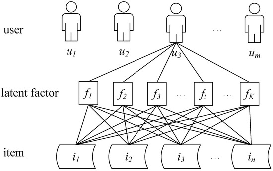
Figure 1.
Rating prediction process based on latent factors. This figure mainly shows the rating prediction process of user for all items.
The solution method for LFM involves minimizing the mean square error. The calculation formula for the loss function is as follows:
where represents a regularization term that is added to prevent overfitting in the model. is an overfitting penalty factor, which is a hyperparameter used to balance the data loss term and the regularization term.
3.2.2. BiasSVD
BiasSVD is an enhanced matrix decomposition method that builds upon singular value decomposition (SVD) [22]. This approach addresses the issue of bias in the user’s ratings for items and establishes a prediction model, as illustrated by the following formula:
where represents the overall mean rating value across all users and items in the user-item rating matrix. denotes the bias term associated with the user u, indicating the rating preference of user u. represents the bias term associated with the item i, reflecting the degree to which item i is preferred by users based on the mean rating value received by the item.
The solution method of bias is also solved by minimizing the mean square error. The loss function calculation formula is as follows:
3.3. LFM-SPE
To assess the efficacy of the proposed SPE method, it is integrated with conventional LFM and BiasSVD models, resulting in the LFM-SPE and BiasSVD-SPE models, respectively. Subsequently, this section presents the procedure for combining the LFM-SPE model.
Utilizing the propensity score to mitigate bias in recommendation systems primarily involves employing inverse propensity weighting. This approach entails assigning weights to the rating data based on the reciprocal of the propensity score, thereby enabling unbiased estimation and mitigating the influence of selection bias within the dataset.
The propensity score is incorporated into the loss function of LFM using the inverse propensity weighting approach, as demonstrated by the following equation:
The loss function is solved using the stochastic gradient descent algorithm [23], which involves the following steps:
Step1. Deriving the parameters and to determine the direction with the steepest gradient descent.
Step2. Iteratively optimizing the parameters through calculations while continuously updating the direction of the steepest decline for each parameter until convergence.
Step3. Obtaining the user implicit semantic preference vector and the product implicit semantic attribute vector , which effectively eliminates selection bias.
Step4. Combining the preference vectors of each user and the attribute vectors of each item to form the user latent semantic preference matrix and the item latent semantic attribute matrix .
By following this iterative process, the LFM-SPE model can effectively learn the latent factors that capture the underlying patterns and preferences in the data, resulting in accurate recommendations. The overall algorithm flow is shown in Algorithm 1.
| Algorithm 1: LFM-SPE Algorithm |
| Input: user-item rating matrix , number of latent factors K, recommended threshold , |
| propensity score threshold D, iterations T |
| 1 Compute based on whether the user has rated the item |
| 2 Compute the propensity score |
| 3 |
| 4 Initialize and randomly |
| 5 for t = 1, …, T do |
| 6 Compute the loss function |
| 7 Compute the derivative of the parameter |
| 8 Update and |
| 9 end |
| 10 Compute the predicted user-item rating matrix |
| Output: the predicted user-item rating matrix |
The approach of incorporating the SPE method into the BiasSVD matrix factorization model is similar to the methodology employed in the LFM-SPE model, where the propensity score is weighted reciprocally in the model’s loss function. Hence, the training process of the BiasSVD-SPE model follows a similar framework and is not explicitly discussed in this section.
4. Experiment
This chapter presents the experiments conducted to evaluate the proposed methodology. Section 4.1 provides an overview of the datasets used in the experiments. Subsequently, Section 4.2 introduces the evaluation indicators employed for assessing the experiment outcomes. Section 4.3 presents the comparative model used in the experiments, and parameter analysis is performed in Section 4.4. Finally, Section 4.5 presents, analyzes, and discusses the experimental results.
4.1. Data Set
To assess the accuracy and effectiveness of the proposed SPE propensity score estimation method in enhancing recommendation performance, a series of experiments were conducted. These experiments utilized three publicly available datasets from MovieLens [24], namely Movielens 100K, Movielens latest, and Movielens 1M, which will be referred to as ML 100K, ML latest, and ML 1M, respectively, for brevity. For each record in the dataset, three features are utilized: user ID, movie ID, and the user’s rating of the movie. An overview of the key statistics for the three datasets is presented in Table 1.

Table 1.
Data set information. The table mainly shows the number of dataset users, items, ratings, and the dataset sparsity.
For each dataset, we randomly selected 80% as training data, 10% as validation data, and the remaining 10% as test data.
4.2. Evaluation Indicators
The prediction accuracy of the model was evaluated using two regression model evaluation metrics: root mean square error and mean absolute error. These metrics provide insights into the performance and accuracy of the predictions.
where represents the test set, denotes the score predicted by the model, and represents the actual score from the test set. The evaluation indicators RMSE and MAE are employed to assess the prediction performance, where smaller values indicate better prediction results.
4.3. Comparison Model
To assess the effectiveness of the SPE propensity score estimation method in mitigating selection bias, we compared it with two baseline models, namely LFM and BiasSVD. Additionally, we included three existing propensity score estimation methods, namely IPS [11], DR [17], and MRDR [18], for comparison. By combining these methods with the LFM model, we constructed three additional comparison models.
LFM-IPS: IPS is a framework for eliminating selection bias, which uses the marginal probability of the user’s item selection as the estimation method of the propensity score and combines the framework and LFM model.
LFM-DR: DR is a dual-robust estimator that integrates the estimation error and the propensity in a doubly robust manner to obtain unbiased performance estimates and mitigates the effect of propensity variance, combining this estimator with an LFM model.
LFM-MRDR: MRDR is a more robust estimator, which further reduces the variance based on the dual robust estimator, combining this estimator with the LFM model.
Considering that the models utilized in this experiment are all founded on matrix decomposition, their time complexity is denoted as O(tmnK). These algorithms exhibit no substantial disparity in terms of time complexity; the variance lies primarily in the number of iterations, while their time consumption remains within the same order of magnitude.
4.4. Parameter Analysis
In the proposed LFM-SPE model presented in this paper, two key parameters significantly impact the recommendation effectiveness of the model: the number of latent factors, , and the recommendation threshold parameter, . In this section, we analyze the impact and variation trends of these two parameters on the recommendation performance individually. Throughout the analysis, while one parameter is examined, the remaining parameters are maintained at their optimal settings.
We set the number of latent factors to , and observed the impact of its changes on the model RMSE and MAE, as shown in Figure 2.
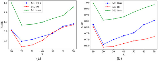
Figure 2.
The impact of the number of hidden factors on the recommendation performance of LFM-SPE model. (a) Impact of on the evaluation index RMSE and (b) impact of on the evaluation index MAE.
The number of latent factors reflects the number of potential association features between users and items. The optimal result obtained by the model depends on whether the appropriate number of hidden factors is selected. As shown in Figure 2, as the value of increases from 10 to 70, the RMSE and MAE indicators show an overall trend of decreasing first and then increasing. This observation demonstrates that as the value of K increases up to a certain threshold, the algorithm’s performance reaches its optimum level. Beyond this threshold, a further increase in the number of hidden factors does not enhance the recommendation effectiveness; instead, it may result in a decline in model performance. This phenomenon can be attributed to overfitting, wherein an excessive number of parameters contribute to suboptimal generalization.
Moreover, we set the recommended threshold parameter to , and observed the impact of its changes on the model RMSE and MAE, as shown in Figure 3.
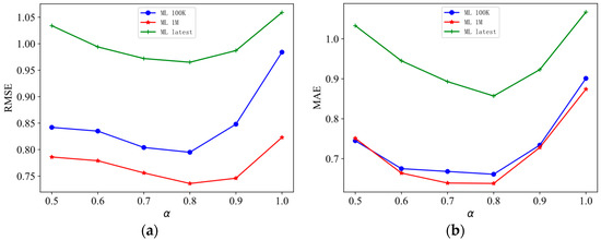
Figure 3.
The impact of recommendation threshold parameter on the recommendation performance of LFM-SPE model. (a) Impact of on the evaluation index RMSE and (b) impact of on the evaluation index MAE.
The recommendation threshold parameter represents the maximum value that the propensity score can reach, and means that 100% of the items appear in the user’s recommendation, which is impossible to observe in the real world. As depicted in Figure 3, when is set to one, both the RMSE and MAE values are significantly higher, indicating a substantial decline in recommendation performance. It is evident that setting the recommendation threshold parameter too high has a detrimental impact on the model’s effectiveness. When is varied from 0.5 to 1, the RMSE and MAE indicators exhibit a decreasing trend initially, followed by an increasing trend. This implies that there exists an optimal value for α that maximizes the recommendation effect. Specifically, when is set to 0.8, the model achieves the best recommendation performance.
Based on the experimental results presented above, it can be concluded that the optimal parameter setting for the recommendation system is a recommended threshold parameter and a number of hidden factors .
4.5. Experimental Results and Discussion
The score prediction results of the proposed LFM-SPE model and BiasSVD-SPE model, along with other comparative models, are presented in Table 2 and Table 3. By analyzing the experimental results, the following conclusions can be drawn.
Table 2.
Comparison of RMSE experimental results of each model.
Table 3.
Comparison of MAE experimental results of each model.
The BiasSVD-SPE model outperforms the BiasSVD matrix factorization algorithm, with an improvement of 2.44% and 3.03% in RMSE and MAE indicators, respectively. Unlike the traditional BiasSVD algorithm, which simply incorporates bias items to account for user and item deviations in score prediction, the BiasSVD-SPE model addresses selection bias by calculating propensity scores for each sample group. It effectively handles selection bias through inverse propensity score weighting, considering variations across different data groups. Consequently, the BiasSVD-SPE model exhibits a more substantial performance enhancement compared to the traditional BiasSVD algorithm as it comprehensively addresses data deviations and offers increased interpretability.
The LFM-SPE model proposed in this paper demonstrates superior recommendation performance compared to other models. When compared to the traditional LFM model, the LFM-SPE model exhibits improvements of 2.00% and 2.97% in the RMSE and MAE evaluation indicators, respectively. Additionally, the recommendation performance of the LFM-IPS, LFM-DR, and LFM-MRDR models, which incorporate propensity scores, also shows enhancement. These findings highlight the significant impact of incorporating propensity scores to mitigate selection bias, leading to substantial improvements in the model’s recommendation performance.
Among the four LFM models with added propensity scores, the LFM-SPE model exhibited the highest recommendation performance. Specifically, the LFM-SPE model outperformed the LFM-IPS model, resulting in improvements of 1.30% and 1.91% in the RMSE and MAE evaluation indicators, respectively. This suggests that the SPE method is superior to IPS in eliminating selection bias. While the IPS algorithm estimates the propensity score based on the marginal probability of user-item selection, the proposed method in this paper simultaneously analyzes and leverages the user and item information, incorporating both the user’s selection rate and the item’s selection preference to estimate the propensity score. As a result, the propensity score estimate is more accurate, leading to improved recommendation performance.
Furthermore, the LFM-SPE model demonstrated slightly better average recommendation performance across the three datasets compared to LFM-MRDR. This indicates that the LFM-MRDR model benefits from the effective reduction of variance through the MRDR double robust estimation method, which in turn mitigates the influence of bias on the recommendation algorithm. It is worth noting that the recommendation effect of LFM-MRDR surpassed that of LFM-DR, further highlighting the efficacy of the MRDR approach.
Overall, the experimental results demonstrate that the LFM-SPE model, with its combined analysis of user and item information and accurate propensity score estimation, outperforms other LFM models with propensity scores in terms of recommendation performance.
5. Conclusions
This paper addresses the issue of selection bias in recommendation systems by introducing the concept of inverse propensity score weighting and proposing a propensity score estimation method called SPE. The SPE method takes into account both user and item information and combines it with traditional matrix factorization-based algorithms, such as LFM and BiasSVD. Experimental evaluations were conducted on the publicly available MovieLens dataset, demonstrating that the SPE method effectively eliminates selection bias and improves recommendation performance. Furthermore, the proposed SPE method outperformed existing propensity score estimation methods.
While the propensity score estimation method presented in this paper has shown improvements in recommendation performance, there are still areas for further enhancement in future research. Firstly, the estimation of propensity scores may introduce high variance issues, and addressing this variance can lead to further performance improvements. Secondly, the methods employed in this paper primarily focus on explicit feedback data, but incorporating implicit feedback data generated by users and items could be explored for bias elimination research.
Overall, the proposed SPE method offers a promising approach to mitigating selection bias in recommendation systems, and future investigations can explore strategies to enhance its performance.
Author Contributions
Conceptualization and methodology, T.M.; data curation and formal analysis, T.M.; experiments and analysis, T.M.; investigation, T.M.; validation and visualization, T.M.; writing—original draft preparation, T.M.; writing—review and editing, T.M. and S.Y.; resources and supervision, S.Y.; funding acquisition, S.Y. All authors have read and agreed to the published version of the manuscript.
Funding
This research was partially supported by the National Science and Technology Program during the Twelfth Five-year Plan Period (2015BAF10B00) and the Science and Technology Innovation Plan Of Shanghai Science and Technology Commission (17511110204).
Institutional Review Board Statement
Not applicable.
Informed Consent Statement
Not applicable.
Data Availability Statement
Not applicable.
Conflicts of Interest
The authors declare no conflict of interest.
References
- Lu, J.; Wu, D.; Mao, M.; Wang, W.; Zhang, G. Recommender system application developments: A survey. Decis. Support Syst. 2015, 74, 12–32. [Google Scholar] [CrossRef]
- Koren, Y. Factorization meets the neighborhood: A multifaceted collaborative filtering model. In Proceedings of the 14th ACM SIGKDD International Conference on Knowledge Discovery and Data Mining, Las Legas, NV, USA, 24–27 August 2008; pp. 426–434. [Google Scholar]
- Chen, J.; Dong, H.; Wang, X.; Feng, F.; Wang, M.; He, X.J. Bias and debias in recommender system: A survey and future directions. ACM Trans. Inf. Syst. 2023, 41, 1–39. [Google Scholar] [CrossRef]
- Abdollahpouri, H.; Mansoury, M.; Burke, R.; Mobasher, B.; Malthouse, E. User-centered evaluation of popularity bias in recommender systems. In Proceedings of the 29th ACM Conference on User Modeling, Adaptation and Personalization, Utrecht, The Netherlands, 21–25 June 2021; pp. 119–129. [Google Scholar]
- Borges, R.; Stefanidis, K. On mitigating popularity bias in recommendations via variational autoencoders. In Proceedings of the 36th Annual ACM Symposium on Applied Computing, Virtual Event, Republic of Korea, 22–26 March 2021; pp. 1383–1389. [Google Scholar]
- Yang, L.; Cui, Y.; Xuan, Y.; Wang, C.; Belongie, S.; Estrin, D. Unbiased offline recommender evaluation for missing-not-at-random implicit feedback. In Proceedings of the 12th ACM Conference on Recommender Systems, Vancouver, BC, Canada, 2 October 2018; pp. 279–287. [Google Scholar]
- Marlin, B.M.; Zemel, R.S. Collaborative prediction and ranking with non-random missing data. In Proceedings of the Third ACM Conference on Recommender Systems, New York, NY, USA, 23–25 October 2009; pp. 5–12. [Google Scholar]
- De Myttenaere, A.; Grand, B.L.; Golden, B.; Rossi, F. Reducing offline evaluation bias in recommendation systems. arXiv 2014, arXiv:1407.0822. [Google Scholar]
- Little, R.J.; Rubin, D.B. Statistical Analysis with Missing Data; John Wiley & Sons: Hoboken, NJ, USA, 2019; Volume 793. [Google Scholar]
- Pradel, B.; Usunier, N.; Gallinari, P. Ranking with non-random missing ratings: Influence of popularity and positivity on evaluation metrics. In Proceedings of the Sixth ACM Conference on Recommender Systems, Dublin, Ireland, 9–13 September 2012; pp. 147–154. [Google Scholar]
- Schnabel, T.; Swaminathan, A.; Singh, A.; Chandak, N.; Joachims, T. Recommendations as treatments: Debiasing learning and evaluation. In Proceedings of the International Conference on Machine Learning, New York, NY, USA, 19–24 June 2016; pp. 1670–1679. [Google Scholar]
- Wang, X.; Zhang, R.; Sun, Y.; Qi, J. Combating selection biases in recommender systems with a few unbiased ratings. In Proceedings of the 14th ACM International Conference on Web Search and Data Mining, Virtual Event, Israel, 8–12 March 2021; pp. 427–435. [Google Scholar]
- Zhang, Q.; Cao, L.; Shi, C.; Hu, L. Tripartite collaborative filtering with observability and selection for debiasing rating estimation on missing-not-at-random data. In Proceedings of the AAAI Conference on Artificial Intelligence, Online, 2–9 February 2021; pp. 4671–4678. [Google Scholar]
- Chen, J.; Wang, C.; Ester, M.; Shi, Q.; Feng, Y.; Chen, C. Social recommendation with missing not at random data. In Proceedings of the 2018 IEEE International Conference on Data Mining (ICDM), Singapore, 17–20 November 2018; pp. 29–38. [Google Scholar]
- Saito, Y. Asymmetric tri-training for debiasing missing-not-at-random explicit feedback. In Proceedings of the 43rd International ACM SIGIR Conference on Research and Development in Information Retrieval, Virtual Event, China, 25–30 July 2020; pp. 309–318. [Google Scholar]
- Saito, Y. Doubly robust estimator for ranking metrics with post-click conversions. In Proceedings of the 14th ACM Conference on Recommender Systems, Virtual Event, 22–26 September 2020; pp. 92–100. [Google Scholar]
- Wang, X.; Zhang, R.; Sun, Y.; Qi, J. Doubly robust joint learning for recommendation on data missing not at random. In Proceedings of the International Conference on Machine Learning, Long Beach, CA, USA, 10–15 June 2019; pp. 6638–6647. [Google Scholar]
- Guo, S.; Zou, L.; Liu, Y.; Ye, W.; Cheng, S.; Wang, S.; Chen, H.; Yin, D.; Chang, Y. Enhanced doubly robust learning for debiasing post-click conversion rate estimation. In Proceedings of the 44th International ACM SIGIR Conference on Research and Development in Information Retrieval, Virtual Event, Canada, 11–15 July 2021; pp. 275–284. [Google Scholar]
- Luo, J.; Liu, D.; Pan, W.; Ming, Z. Unbiased recommendation model based on improved propensity score estimation. J. Comput. Appl. 2021, 41, 3508. [Google Scholar]
- Saito, Y.; Yaginuma, S.; Nishino, Y.; Sakata, H.; Nakata, K. Unbiased recommender learning from missing-not-at-random implicit feedback. In Proceedings of the 13th International Conference on Web Search and Data Mining, Houston, TX, USA, 3–7 February 2020; pp. 501–509. [Google Scholar]
- Koren, Y.; Bell, R.; Volinsky, C. Matrix factorization techniques for recommender systems. Computer 2009, 42, 30–37. [Google Scholar] [CrossRef]
- Sarwar, B.; Karypis, G.; Konstan, J.; Riedl, J. Application of Dimensionality Reduction in Recommender System—A Case Study; Minnesota University Minneapolis Department of Computer Science: Minneapolis, MN, USA, 2000. [Google Scholar]
- Ling, G.; Yang, H.; King, I.; Lyu, M.R. Online learning for collaborative filtering. In Proceedings of the 2012 International Joint Conference on Neural Networks (IJCNN), Brisbane, Australia, 10–15 June 2012; pp. 1–8. [Google Scholar]
- Harper, F.M.; Konstan, J.A. The movielens datasets: History and context. ACM Trans. Interact. Intell. Syst. 2015, 5, 1–19. [Google Scholar] [CrossRef]
Disclaimer/Publisher’s Note: The statements, opinions and data contained in all publications are solely those of the individual author(s) and contributor(s) and not of MDPI and/or the editor(s). MDPI and/or the editor(s) disclaim responsibility for any injury to people or property resulting from any ideas, methods, instructions or products referred to in the content. |
© 2023 by the authors. Licensee MDPI, Basel, Switzerland. This article is an open access article distributed under the terms and conditions of the Creative Commons Attribution (CC BY) license (https://creativecommons.org/licenses/by/4.0/).