Article

scCGImpute: An Imputation Method for Single-Cell RNA Sequencing Data Based on Similarities between Cells and Relationships among Genes

School of Mathematics and Physics, Wuhan Institute of Technology, Wuhan 430205, China
*
Author to whom correspondence should be addressed.
Appl. Sci. 2023, 13(13), 7936; https://doi.org/10.3390/app13137936
Submission received: 20 May 2023 / Revised: 2 July 2023 / Accepted: 4 July 2023 / Published: 6 July 2023

Abstract

:
Single-cell RNA sequencing (scRNA-seq) has become a powerful technique to investigate cellular heterogeneity and complexity in various fields by revealing the gene expression status of individual cells. Despite the undeniable benefits of scRNA-seq, it is not immune to its inherent limitations, such as sparsity and noise, which would hinder downstream analysis. In this paper, we introduce scCGImpute, a model-based approach for addressing the challenges of sparsity in scRNA-seq data through imputation. After identifying possible dropouts using mixed models, scCGImpute takes advantage of the cellular similarity in the same subpopulation to impute and then uses random forest regression to obtain the final imputation. scCGImpute only imputes the likely dropouts without changing the non-dropout data and can use information from the similarity of cells and genetic correlation simultaneously. Experiments on simulation data and real data were made, respectively, to evaluate the performance of scCGImpute in terms of gene expression recovery and clustering analysis. The results demonstrated that scCGImpute can effectively restore gene expression and improve the identification of cell types.

1. Introduction

Single-cell RNA sequencing has become increasingly popular in transcriptome research [1] owing to its ability to reveal gene expression at single-cell resolution [2], which can help researchers study cellular heterogeneity and complexity. This technology has been applied to many areas, such as the classification of novel cell subtypes [3,4,5], differential gene expression analysis [6,7], spatial reconstruction [8,9], and development trajectories [10,11].
Compared to bulk RNA sequencing, single-cell RNA sequencing has higher resolution, which can better reflect the heterogeneity across cells. However, the single-cell transcriptome sequencing data is sparse due to the low starting amount of transcripts, which increases the likelihood of missed transcripts during the reverse transcription steps [12,13]. Thus, the transcripts cannot be detected in the later step of sequencing, resulting in the count appearing as zero, which is called the dropout event. Specifically, some genes are expressed in some cells but not in others of the same type. It is necessary to note that not all zeros in single-cell RNA data can be considered dropout values. A zero value for a gene in a cell could be biological zeros, which mean the true absence of transcripts or mRNAs. The biological zeros can be produced by cell type-specific expression or by the phenomenon that many genes are transcribed intermittently [14,15]. Furthermore, the scRNA-seq platform used, the depth of sequencing, and the potential expression level of the gene can influence the degree of sparsity [16]. The generation of biological and non-biological zeros results in a proportion of zeros in the scRNA-seq data as high as 90% [17], which poses challenges for downstream computational analyses [13]. To better perform downstream analysis, it is necessary to impute the scRNA-Seq data.
Several scRNA-seq-specific imputation methods from multiple angles have been proposed to solve the problem of sparsity and improve downstream analysis. According to Lähnemann D. et al. [16], it can be divided into three categories without external reference. The three categories include model-based imputation methods [17,18,19,20,21], data-smoothing methods [22,23], and data-reconstruction methods [24,25,26,27,28]. Model-based imputation methods assume that the scRNA-seq data conform to a distribution. Based on the properties of scRNA-seq data, some models are designed to model the distribution of the scRNA-seq data, such as decreasing logistic function [18], Gamma-Normal mixed model [19], negative binomial (NB) model [17], zero-inflated negative binomial (ZINB) model [21], and so on. Data-smoothing methods impute the data using information from similar cells. They are usually imputed with zero values. Data-reconstruction methods usually use matrix decomposition [24,25] or machine learning methods [26,27,28] to reconstruct data and these three methods usually overlap. Most of these methods impute the data by leveraging information on the similarity of cells or the correlations of genes. For instance, after detecting possible dropout values using the Gamma-Normal mixed distribution model, scImpute [19] takes advantage of information among similar cells to impute the data through non-negative least squares regression. VIPER [20] preserves gene expression by leveraging information from cells with similar expression patterns rather than using information from the same subpopulation, which uses a sparse non-generative regression model to actively select the sparse set of local neighborhood cells that are most predictive of the cells to be imputed. DeepImpute [26] employs a deep neural network along with dropout layers and a loss function, using information from correlated genes to learn patterns for imputing “target genes.” DeepImpute adopted a dive-and-conquer strategy in the deep learning imputation process for its efficiency by constructing multiple sub-neural networks. scRecover [21] assumes that scRNA-seq data follows the ZINB distribution. After distinguishing between true zeros and dropout zeros, scRecover applied the result to existing imputation methods to impute. Several approaches also take advantage of both cell-level and gene-level information. For example, SAVER [17] assumes that the count of each gene in each cell follows a Poison-Gamma mixed distribution, also known as the NB model. SAVER performs Poisson LASSO regression between the genes to estimate the prior mean, and then, after estimating the prior variance, SAVER uses the posterior mean derived from the posterior distribution of the true expression as the recovered expression value. However, if SAVER adjusts all gene expression levels, it may introduce new biases and eliminate biological zeros. MAGIC [22] shares information across similar cells through data diffusion to denoise the cell count matrix and impute missing values. Like SAVER, MAGIC adjusts all gene expression levels. Some methods, such as scRMD [24] and ALRA [25], do not use the information between genes or cells but reconstruct data matrices for imputation. scRMD models the dropout imputation problem as a robust matrix decomposition based on the low-rankness assumption and the sparsity assumption. ALRA selectively computes technical zeros using the nonnegative and low-rank structure of the gene expression matrix. ALRA first computes the low-rank approximation of the data matrix using singular vector decomposition (SVD). The biological zeros in the matrix are then restored by thresholding the entries of the matrix. In addition, a few methods incorporate external references to the current datasets [29,30,31,32].
Here, we propose a model-based imputation algorithm that borrows information from similar cells and related genes simultaneously. The framework of scCGImpute is presented in Figure 1. Firstly, the gene expression matrix is preprocessed with library size normalization and logarithmic transformation. Secondly, the preprocessed scRNA-seq data profile is used for PCA dimension reduction and spectral clustering. Thirdly, after the clustering results are obtained for each subpopulation, the Gamma-Normal mixing model is used to identify the dropout value of each gene. And then the average of the high confidence part for each gene in each subpopulation is used as the imputed value of the low confidence part. The imputation results obtained by cell similarity are used to calculate the relationships between genes in each subpopulation. Finally, based on the data that already contained information on cell similarity in the previous step, for each gene in each subpopulation, the highly related genes are selected for the random forest regression. Thus, scCGImpute preserves heterogeneity across cells. And we used the above eight methods from different angles with scCGImpute to do the cluster analysis. They are model-based imputation methods scImpute (Gamma-Normal mixed model), SAVER (NB model), scRecover (ZINB model), and VIPER (Sparse non-negative regression model), data-smoothing methods MAGIC, matrix decomposition methods in data reconstruction scRMD and ALRA, and machine learning methods in data reconstruction DeepImpute. By comparing the results on the simulated data and the real datasets, it is proven that scCGImpute can recover gene expression and promote the recognition of cell subpopulations.

2. Materials and Methods

2.1. Data Preprocessing

The input matrix X (g × n) is a count matrix with g genes and n cells. Firstly, the genes with a mean expression of less than 0.001 and non-zero expression of fewer than three cells were removed because of the high dropout rate of scRNA-seq data. Secondly, we normalized the matrix X by the library size of each cell to eliminate the effect of sequencing depth; this standardized approach is called CPM. After CPM normalization, some data were very large and some were very small. Therefore, the log transformation with pseudo-count 1.01 was then performed to prevent subsequent processing from being affected by the large values. Specifically, we define the normalized and log-transformed matrix as Y = y i j g × n , and we set
y i j = l o g 10 x i j i = 1 g x i j × 1,000,000 + 1.01   ,   i = 1,2 , , g , j = 1,2 , , n

2.2. Dimension Reduction and Clustering

After preprocessing the data, dimension reduction and clustering were used based on matrix Y to leverage the similarity among cells of the same type and the correlations between genes for imputing the single-cell RNA-seq data. Before dimensionality reduction, genes with a mean value greater than 1 and a variation coefficient greater than the upper quartile were selected for dimension reduction in order to select highly variable genes to achieve better clustering results. The dimension reduction can remove noise and unimportant features, thus achieving the purpose of improving the data processing speed. We used PCA to reduce the dimension of the matrix and designated the matrix after dimension reduction as H, which was then used to compute the distance matrix D between cells to remove outliers. For each cell j, the closest cell can be found according to the distance matrix D. Then we set the closest distance for cell j as m j , thus we can get the set M = { m 1 , m 2 , , m n } . Individual cells may be outliers due to the presence of excessive zeros resulting from both technical and biological factors, which can lead to a lack of expression information or contain biological information. Before clustering and the subsequent process, the outliers were detected and removed. Outliers are cells with no neighboring cells whose closest distance m j is greater than the upper quartile plus 1.5 times the quartile distance of set M. After removing outliers, spectral clustering is selected to cluster the reduced dimension matrix H, as it is more adaptable to different data distributions. The number of clusters, k, can be set to the desired number. Through these processes, we obtained k-cell subpopulations and removed the outliers.

2.3. Imputation Strategy

For each gene i in each cell subpopulation k, the Gamma-Normal mixed model was used to identify dropout values. We divided gene i into a high-confidence cell set A and a low-confidence cell set B based on the dropout probability, and its expression value is modeled as a random variable Z i ( k ) with the following density function:
f Z i ( k ) ( z ) = δ i ( k ) G a m m a ( z ; α i ( k ) , β i ( k ) ) + ( 1 δ i ( k ) ) N o r m a l ( z ; μ i ( k ) , σ i ( k ) )
where δ i ( k ) is the dropout rate in cell subpopulation k of gene i, α i ( k ) , β i ( k ) are parameters of Gamma distribution, μ i ( k ) , σ i ( k ) are parameters of Normal distribution. And the dropout probability p i j can be calculated by the following formula:
p i j = δ i k ^ G a m m a Z i j ; α i k ^ , β i k ^ δ i k ^ G a m m a Z i j ; α i k ^ , β i k ^ + 1 δ i k ^ N o r m a l Z i j ; μ i k ^ , σ i k ^
where α i ( k ) ^ , β i ( k ) ^ , μ i ( k ) ^ , σ i ( k ) ^ and δ i ( k ) ^ are estimated by Expectation–Maximization (EM) algorithm, and the dropout probability p i j represents the dropout rate of the gene i in the cell j. After getting the dropout probability, for each gene i in each cell subpopulation k, the dropout values are identified by the Gamma-Normal mixed model. The data with a dropout probability higher than 0.5 are considered to be low confidence set B, which needs to be imputed, and conversely, the data with a dropout probability lower than or equal to 0.5 are considered to be high confidence set A. After obtaining the high confidence set A and the low confidence set B for each cell subpopulation k, we imputed the data in two steps. In the following two steps, the high confidence set A and the low confidence set B for each gene i are unchanged.
  • For each gene i, the data in set A were averaged, and its average value was used as the imputation of gene i in low confidence set B. We denoted the imputation matrix as Y. The information across cells was already incorporated into matrix Y at this stage, but this is not the final imputation. And then, correlations between genes are calculated by the Pearson correlation coefficient for each cell subpopulation. The genes with an absolute value of the correlation coefficient greater than 0.5 were selected for the next step of the calculation.
  • For each gene i, as shown in Figure 2, based on the matrix Y and the high correlation genes we filter out, random forest regression is used for regression training on data with high confidence cells. Then, predictions are made for data with low confidence cells. Thus, it preserves the heterogeneity across cells and does not impute all zeros. At the beginning of the regression with random forest, the low confidence set B is imputed with information from similar cells. When the gene i which has been predicted by random forest regression, is used to calculate other genes, the gene expression level of gene i corresponds to the value predicted by random forest; that is, after calculating gene i, the set B of gene i is retained for the subsequent random forest regression of the next gene. The random forest regression model establishes several uncorrelated decision trees by randomly extracting samples and features. Each decision tree can obtain a prediction result based on the extracted samples and features. The regression model of the whole forest can be obtained by taking the average value of all the results. Using random forests, we can learn nonlinear relationships between genes.

2.4. Evaluation Strategies of Clustering

To evaluate the clustering results, we selected three evaluation indicators: adjusted Rand index (ARI), normalized mutual information (NMI), and purity. These are three evaluation indicators designed from different perspectives. Each indicator has its own advantages and disadvantages, so we stack the three indicators as the final cluster evaluation results.
The adjusted Rand index solved the problem of RI, which cannot guarantee a randomly divided clustering result close to 0. Let n i j be the number in both real label i and cluster j. The adjusted Rand index can be calculated as follows:
A R I = R I E ( R I ) max R I E ( R I )
where E(RI) is the expected value of RI, which is E i , j n i j 2 = i n i . 2 j n . j 2 / n 2 . The ARI ranges from −1 to 1.
The normalized mutual information measures the similarity between clustering results and real labels from the perspective of information entropy. The normalized mutual information can be calculated as follows:
N M I = 2 I ( C ; T ) H C + H ( T )
where C and T are defined as the predicted clustering result and the true category, respectively. I(C; T) is the mutual entropy, and H(C) and H(T) are the information entropy of C and T, respectively. The NMI ranges from 0 to 1.
The purity can be calculated as follows:
1 N i m a x j | c i t j |
where N is the total number of samples, c i represents cluster i and t j represents category j. The purity ranges from 0 to 1.

2.5. Simulate scRNA-Seq Data

Splat builds on the negative binomial distribution (or Gamma-Poisson distribution) to simulate RNA-seq data. Splat simulation can capture many features observed in real scRNA-Seq data, including trended gene-wise dispersion, zero inflation, differing library sizes between cells, and high expression outlier genes [33]. We used splatSimulateGroups() function in the splatter to simulate the scRNA-Seq data of three cell subpopulations with a size of 300 cells and 1000 genes per cell. We set group.prob (the probability of a cell being assigned to a group) to c (0.3, 0.3, 0.4), de.prob (the probability that a gene is selected for differential expression) to 0.1, and set dropout.mid (a parameter that controls the point at which the probability is equal to 0.5) from 0 to 4.5 in increments of 0.5 each time. We retained the default values for other parameters.

2.6. Real Data Used to Evaluate Clustering Result

We used four real data sets to evaluate the performance of scCGImpute with eight other methods for identifying cell types. The information for these four data sets is shown in Table 1, where the number of genes and dropout rate are the results after pre-processing.

3. Results

The effectiveness of single-cell imputation methods is usually evaluated in two aspects: one is whether it restores gene expression, and the other is whether it helps in downstream analysis. For the first aspect, we used the simulation data to calculate the correlation between the raw data and the scCGImpute imputation and the reference data, and we used the real data set Ziegenhain to calculate the correlation between the raw data and the scCGImpute imputation and the known concentration. For the second aspect, we evaluated the clustering results using simulated data and four real datasets with sizes as small as 30 and as large as 3005, where the simulated data simulated the dropout rate at a minimum of about 20% to a maximum of about 80%.

3.1. Simulation Analysis

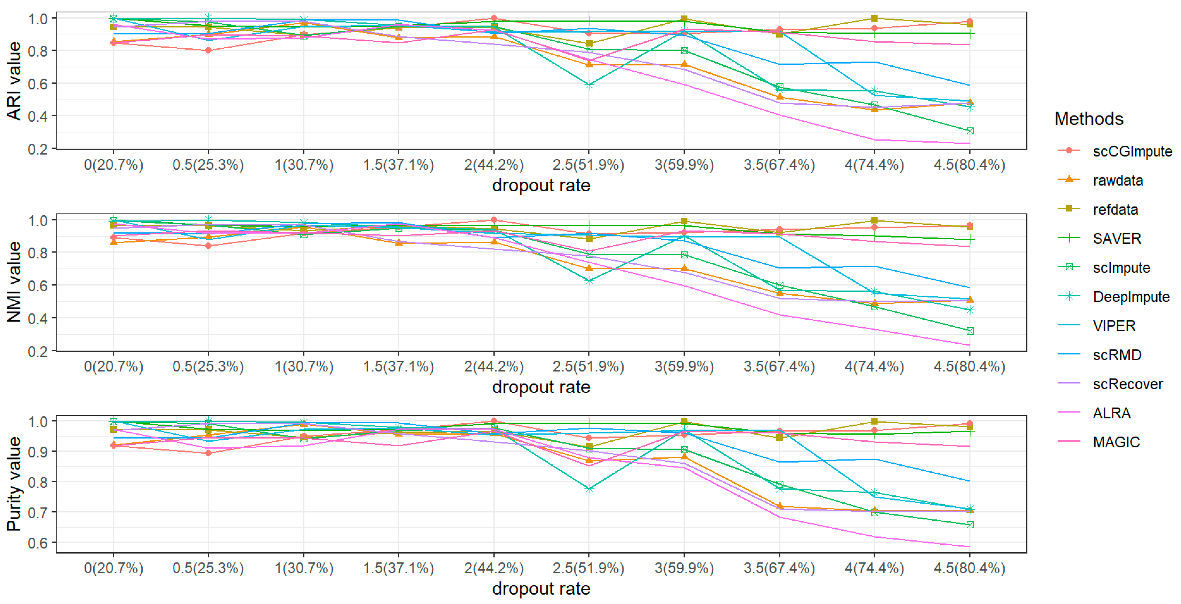
We compared the performance of scCGImpute with eight other methods using a simulation of the dataset generated by splatter, consisting of 1000 genes and 300 cells. The details of the parameters are in the methods. We referred to the data before dropout as reference data and the data after dropout as raw data. We used this simulated data to compare the clustering performance of scCGImpute and other methods. Since there are only 1000 genes in the simulation, we used spectral clustering to cluster them directly. ARI, NMI, and purity were selected to evaluate clustering performance, and the results are shown in Figure 3. It can be found that scCGImpute has more accurate clustering results than other methods for all three indexes on this simulated data. As the dropout rate increases, scCGImpute can still maintain good clustering performance. Even at a dropout rate of 80%, scCGImpute can still have a good clustering effect. The next closest methods are SAVER and MAGIC, while the performance of other methods shows a significant reduction.
We also calculated the Pearson correlations for reference data with raw data and scCGImpute imputation on the cell level and on the gene level and presented the results in a box diagram. The correlation between scCGImpute imputation and the raw data with reference data was calculated for each dropout rate, as shown in Figure 4. Although there was no significant change in the cell correlation, scCGImpute showed a significant improvement in the gene correlation compared with raw data. While it was not significant at 0.5 dropout.mid, the median value was still higher than the raw data.

3.2. scCGImpute Recovers Gene Expression in Real Data

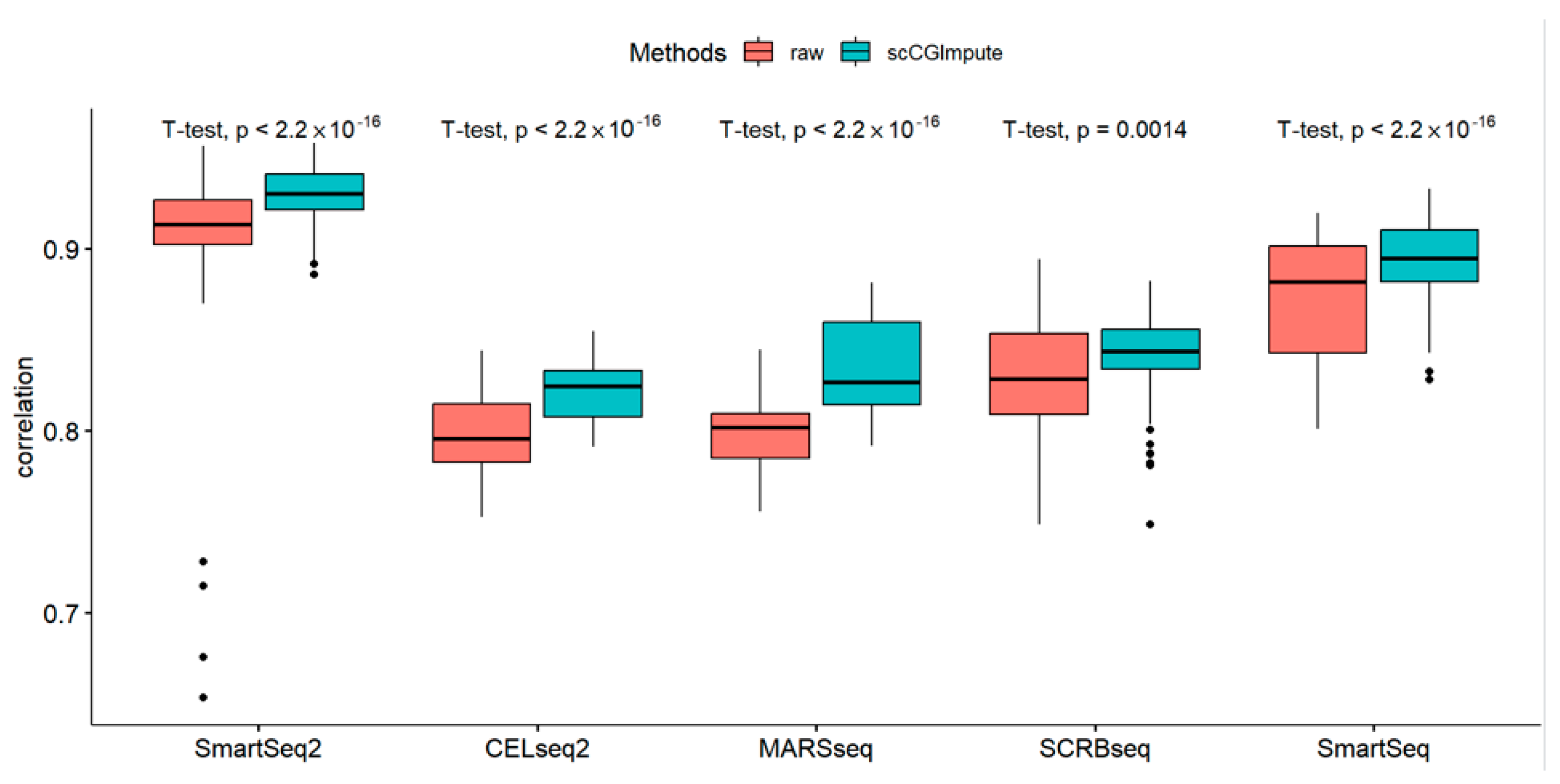
We use the Ziegenhain scRNA-seq data [37] to evaluate the resilience to the dropout events of scCGImpute. The Ziegenhain dataset is generated from 583 mouse embryonic stem cells sequenced using six different RNA-Seq protocols. The data generated by five sequencing methods, which contained 92 synthetic RNA molecules designed by the External RNA Controls Consortium (ERCC), were selected to be imputed. The imputation of ERCC genes was then compared with the known concentration of ERCCs using Pearson correlation analysis. The ERCCs are a group of external RNA control substances with known sequences and known concentration levels that can be used as reference standards in gene expression experiments. The results are shown in Figure 5. Compared with the original data generated by the five sequencing methods, the correlation between scCGImpute and the known concentrations of ERCCs is improved and significantly different from the original data.

3.3. scCGImpute Enhances the Ability to Identify Cell Types in Real Data

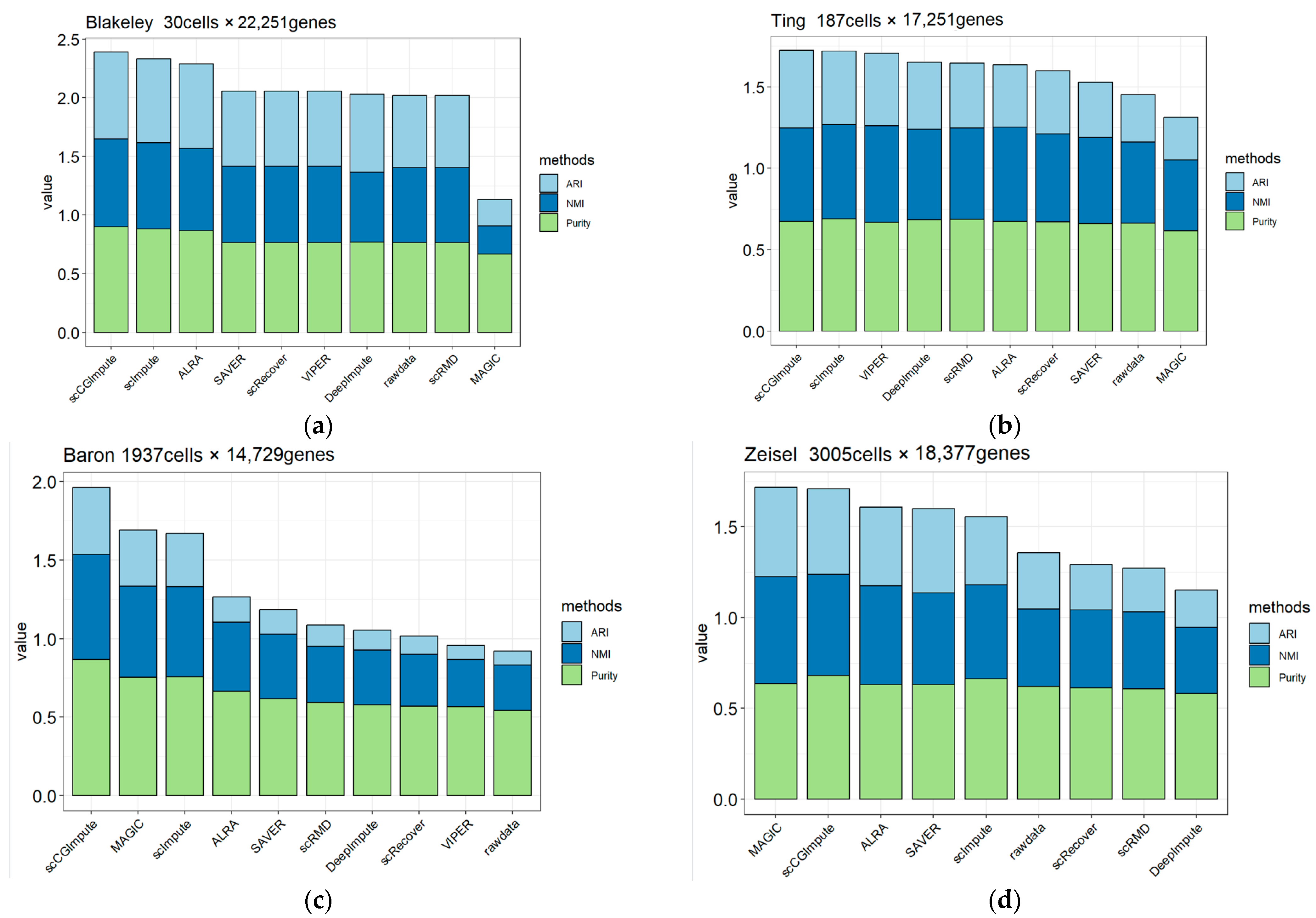
In this section, four real datasets (Blakeley [34], Ting [35], Baron [36], and Zeisel [4]) are used to evaluate the ability to recognize cell types in scCGImpute. The smallest dataset consists of 30 cells, and the largest dataset contains 3005 cells. The three clustering evaluation indexes (ARI, NMI, and Purity) are selected to evaluate the results of identifying cell types. We used the cell type label of these data only for evaluating the clustering results and not for identifying cell types. The details of the pre-processing can be found in the methods. The clustering performance of the original data, the imputations of scCGImpute and other eight methods are shown in Figure 6. And the results of these three indicators are presented in a stacked way. In addition, VIPER failed to run on the Zeisel dataset for a day, so we don’t show it. Among these four real datasets, compared with the original data and the data imputed by the other eight methods, scCGImpute could obtain better clustering results regardless of whether the data set was small or large. While MAGIC performs better than scCGImpute in the Zeisel dataset, scCGImpute significantly outperforms MAGIC in the other three datasets. This can be attributed to the suitability of MAGIC for large datasets. Nevertheless, the peculiarity of MAGIC’s ability to adjust all gene expression levels may introduce new bias into the data. In Table 1, it can be observed that the Baron dataset has the highest dropout rate, reaching 86.9%. The performance of scCGImpute on the Baron dataset, along with the cluster analysis results of the simulate dataset, mutually confirm that scCGImpute can perform well even when dealing with high dropout rates.

4. Discussion

Single-cell RNA sequencing is a powerful tool to study cell heterogeneity; however, its sparsity could hinder downstream analysis. To address this problem, we propose an imputation method called scCGImpute to recover gene expression and help improve downstream analysis. scCGImpute performs spectral clustering on the data that has been reduced in dimension and then uses the Gamma-Normal hybrid model to obtain dropout values set for each gene in each type. We use the averages of high-confidence cells in the same subpopulation as the initial imputation for low-confidence cells. The final imputation is then obtained through regression using random forests based on the initial imputation. The advantage of scCGImpute is that it uses both cell-to-cell similarity and gene-to-gene correlation to impute the scRNA-seq data while preserving the variability across cells. In addition, scCGImpute does not impute all zeros, which avoids the wrong imputation of biological zeros to a certain extent. The experiments of gene expression recovery and clustering analysis were performed on simulate and real data, and the results show that scCGImpute can recover gene expression and improve the result of cluster analysis more effectively than other methods. In the cluster analysis, scCGImpute was compared with eight methods designed from different perspectives, four of which were different model-based methods, and the experiment result shows that scCGImpute had better improvement than the other methods in the cluster analysis. In addition, in the simulated data, Splat is modeled based on the NB model, while scCGImpute is based on the Gamma-Normal mixed model. Furthermore, scCGImpute can also perform well, which proves that scCGImpute is robust to model distribution. Moreover, scCGImpute seems to be very good at handling scRNA-seq data with a high dropout rate. Even when the dropout rate exceeds 80%, scCGImpute can also achieve a good clustering effect.
Even though scCGImpute already has good performance, there are still some areas that can be improved. First of all, since the size of the current scRNA-seq data has reached millions of cells, the computational complexity of dimensionality reduction by PCA will become higher and higher with the increase in the dataset. Although random PCA can be used when the dataset is too large, problems such as insufficient memory may still occur. To solve this problem, we can do feature extraction before working with big data, or use a distributed computing framework. Secondly, many people think that the data distribution of RNA-Seq is more consistent with the Poisson-Gamma distribution, so we can also use the Gamma-Poisson distribution to calculate the dropout rate of the data. In the future, we will pay attention to these questions and hope to achieve an approach that works better with large datasets.

Author Contributions

Methodology, T.L. and Y.L.; software, T.L.; data curation, T.L.; writing—original draft, T.L. and Y.L.; supervision, Y.L. All authors have read and agreed to the published version of the manuscript.

Funding

This work was supported by the National Natural Science Foundation of China (Grant No. 12001408).

Institutional Review Board Statement

Not applicable.

Informed Consent Statement

Not applicable.

Data Availability Statement

The dataset Blakeley is available at Gene Expression Omnibus (GEO) under accession code GSE66507. The dataset Ting is available at GEO under accession code GSE51372. The dataset Baron is available at GEO under accession code GSM2230757. The dataset Zeisel is available at http://linnarssonlab.org/cortex/, accessed on 2 November 2022. The Ziegenhain dataset is available at GEO under accession code GSE75790. The code for the paper is available at https://github.com/Liutto/scCGImpute, accessed on 7 May 2022.

Conflicts of Interest

The authors declare no conflict of interest.

References

  1. Jovic, D.; Liang, X.; Zeng, H.; Lin, L.; Xu, F.; Luo, Y. Single-cell RNA sequencing technologies and applications: A brief overview. Clin. Transl. Med. 2022, 12, e694. [Google Scholar] [CrossRef] [PubMed]
  2. Tang, F.; Barbacioru, C.; Wang, Y.; Nordman, E.; Lee, C.; Xu, N.; Surani, M.A. mRNA-Seq whole-transcriptome analysis of a single cell. Nat. Methods 2009, 6, 377–382. [Google Scholar] [CrossRef] [PubMed]
  3. Grün, D.; Lyubimova, A.; Kester, L.; Wiebrands, K.; Basak, O.; Sasaki, N.; Clevers, H.; van Oudenaarden, A. Single-cell messenger RNA sequencing reveals rare intestinal cell types. Nature 2015, 525, 251–255. [Google Scholar] [CrossRef] [PubMed]
  4. Zeisel, A.; Muñoz-Manchado, A.B.; Codeluppi, S.; Lönnerberg, P.; La Manno, G.; Juréus, A.; Marques, S.; Munguba, H.; He, L.; Betsholtz, C.; et al. Cell types in the mouse cortex and hippocampus revealed by single-cell RNA-seq. Science 2015, 347, 1138–1142. [Google Scholar] [CrossRef]
  5. Keren-Shaul, H.; Spinrad, A.; Weiner, A.; Matcovitch-Natan, O.; Dvir-Szternfeld, R.; Ulland, T.K.; David, E.; Baruch, K.; Lara-Astaiso, D.; Toth, B.; et al. A Unique Microglia Type Associated with Restricting Development of Alzheimer’s Disease. Cell 2017, 169, 1276–1290.e17. [Google Scholar] [CrossRef] [Green Version]
  6. Kim, K.T.; Lee, H.W.; Lee, H.O.; Kim, S.C.; Seo, Y.J.; Chung, W.; Park, W.Y. Single-cell mRNA sequencing identifies subclonal heterogeneity in anti-cancer drug responses of lung adenocarcinoma cells. Genome Biol. 2015, 16, 127. [Google Scholar] [CrossRef] [Green Version]
  7. Finak, G.; McDavid, A.; Yajima, M.; Deng, J.; Gersuk, V.; Shalek, A.K.; Gottardo, R. MAST: A flexible statistical framework for assessing transcriptional changes and charac-terizing heterogeneity in single-cell RNA sequencing data. Genome Biol. 2015, 16, 278. [Google Scholar] [CrossRef] [Green Version]
  8. Satija, R.; A Farrell, J.; Gennert, D.; Schier, A.F.; Regev, A. Spatial reconstruction of single-cell gene expression data. Nat. Biotechnol. 2015, 33, 495–502. [Google Scholar] [CrossRef] [Green Version]
  9. Qian, J.; Liao, J.; Liu, Z.; Chi, Y.; Fang, Y.; Zheng, Y.; Shao, X.; Liu, B.; Cui, Y.; Guo, W.; et al. Reconstruction of the cell pseudo-space from single-cell RNA sequencing data with scSpace. Nat. Commun. 2023, 14, 2484. [Google Scholar] [CrossRef]
  10. Moignard, V.; Woodhouse, S.; Haghverdi, L.; Lilly, A.J.; Tanaka, Y.; Wilkinson, A.C.; Buettner, F.; Macaulay, I.C.; Jawaid, W.; Diamanti, E.; et al. Decoding the regulatory network of early blood development from single-cell gene expression measurements. Nat. Biotechnol. 2015, 33, 269–276. [Google Scholar] [CrossRef] [Green Version]
  11. Herring, C.A.; Banerjee, A.; McKinley, E.T.; Simmons, A.J.; Ping, J.; Roland, J.T.; Franklin, J.L.; Liu, Q.; Gerdes, M.J.; Coffey, R.J.; et al. Unsupervised Trajectory Analysis of Single-Cell RNA-Seq and Imaging Data Reveals Alternative Tuft Cell Origins in the Gut. Cell Syst. 2018, 6, 37–51.e9. [Google Scholar] [CrossRef] [PubMed] [Green Version]
  12. Zhang, L.; Zhang, S. Comparison of computational methods for imputing single-cell RNA-sequencing data. IEEE/ACM Trans. Comput. Biol. Bioinform. 2018, 17, 376–389. [Google Scholar] [CrossRef] [PubMed]
  13. Kharchenko, P.V.; Silberstein, L.; Scadden, D.T. Bayesian approach to single-cell differential expression analysis. Nat. Methods 2014, 11, 740–742. [Google Scholar] [CrossRef] [PubMed]
  14. Eraslan, G.; Simon, L.M.; Mircea, M.; Mueller, N.S.; Theis, F.J. Single-cell RNA-seq denoising using a deep count autoencoder. Nat. Commun. 2019, 10, 390. [Google Scholar] [CrossRef] [PubMed] [Green Version]
  15. Jiang, R.; Sun, T.; Song, D.; Li, J.J. Statistics or biology: The zero-inflation controversy about scRNA-seq data. Genome Biol. 2022, 23, 31. [Google Scholar] [CrossRef]
  16. Lähnemann, D.; Köster, J.; Szczurek, E.; McCarthy, D.J.; Hicks, S.C.; Robinson, M.D.; Vallejos, C.A.; Campbell, K.R.; Beerenwinkel, N.; Mahfouz, A.; et al. Eleven grand challenges in single-cell data science. Genome Biol. 2020, 21, 31. [Google Scholar] [CrossRef]
  17. Huang, M.; Wang, J.; Torre, E.; Dueck, H.; Shaffer, S.; Bonasio, R.; Murray, J.I.; Raj, A.; Li, M.; Zhang, N.R. SAVER: Gene expression recovery for single-cell RNA sequencing. Nat. Methods 2018, 15, 539–542. [Google Scholar] [CrossRef]
  18. Lin, P.; Troup, M.; Ho, J.W.K. CIDR: Ultrafast and accurate clustering through imputation for single-cell RNA-seq data. Genome Biol. 2017, 18, 59. [Google Scholar] [CrossRef] [Green Version]
  19. Li, W.V.; Li, J.J. An accurate and robust imputation method scImpute for single-cell RNA-seq data. Nat. Commun. 2018, 9, 997. [Google Scholar] [CrossRef] [Green Version]
  20. Chen, M.; Zhou, X. VIPER: Variability-preserving imputation for accurate gene expression recovery in single-cell RNA se-quencing studies. Genome Biol. 2018, 19, 196. [Google Scholar] [CrossRef]
  21. Miao, Z.; Li, J.; Zhang, X. scRecover: Discriminating true and false zeros in single-cell RNA-seq data for imputation. BioRxiv 2019, 665323. [Google Scholar] [CrossRef] [Green Version]
  22. Van Dijk, D.; Sharma, R.; Nainys, J.; Yim, K.; Kathail, P.; Carr, A.J.; Pe’er, D. Faculty Opinions recommendation of Recovering Gene Interactions from Single-Cell Data Using Data Diffusion. Cell 2018, 174, 716–729.e27. [Google Scholar] [CrossRef] [Green Version]
  23. Gong, W.; Kwak, I.-Y.; Pota, P.; Koyano-Nakagawa, N.; Garry, D.J. DrImpute: Imputing dropout events in single cell RNA sequencing data. BMC Bioinform. 2018, 19, 220. [Google Scholar] [CrossRef] [Green Version]
  24. Chen, C.; Wu, C.; Wu, L.; Wang, X.; Deng, M.; Xi, R. scRMD: Imputation for single cell RNA-seq data via robust matrix decomposition. Bioinformatics 2020, 36, 3156–3161. [Google Scholar] [CrossRef] [PubMed]
  25. Linderman, G.C.; Zhao, J.; Roulis, M.; Bielecki, P.; Flavell, R.A.; Nadler, B.; Kluger, Y. Zero-preserving imputation of single-cell RNA-seq data. Nat. Commun. 2022, 13, 192. [Google Scholar] [CrossRef] [PubMed]
  26. Arisdakessian, C.; Poirion, O.; Yunits, B.; Zhu, X.; Garmire, L.X. DeepImpute: An accurate, fast, and scalable deep neural network method to impute single-cell RNA-seq data. Genome Biol. 2019, 20, 211. [Google Scholar] [CrossRef] [PubMed] [Green Version]
  27. Xu, Y.; Zhang, Z.; You, L.; Liu, J.; Fan, Z.; Zhou, X. scIGANs: Single-cell RNA-seq imputation using generative adversarial networks. Nucleic Acids Res. 2020, 48, e85. [Google Scholar] [CrossRef] [PubMed]
  28. Wang, J.; Ma, A.; Chang, Y.; Gong, J.; Jiang, Y.; Qi, R.; Wang, C.; Fu, H.; Ma, Q.; Xu, D. scGNN is a novel graph neural network framework for single-cell RNA-Seq analyses. Nat. Commun. 2021, 12, 1882. [Google Scholar] [CrossRef] [PubMed]
  29. Peng, T.; Zhu, Q.; Yin, P.; Tan, K. SCRABBLE: Single-cell RNA-seq imputation constrained by bulk RNA-seq data. Genome Biol. 2019, 20, 88. [Google Scholar] [CrossRef] [Green Version]
  30. Ronen, J.; Akalin, A. netSmooth: Network-smoothing based imputation for single cell RNA-seq. bioRxiv 2017, 234021. [Google Scholar] [CrossRef]
  31. Wang, J.; Agarwal, D.; Huang, M.; Hu, G.; Zhou, Z.; Ye, C.; Zhang, N.R. Data denoising with transfer learning in single-cell transcriptomics. Nat. Methods 2019, 16, 875–878. [Google Scholar] [CrossRef] [PubMed]
  32. Chen, S.; Yan, X.; Zheng, R.; Li, M. Bubble: A fast single-cell RNA-seq imputation using an autoencoder constrained by bulk RNA-seq data. Briefings Bioinformat. 2023, 24, bbac580. [Google Scholar] [CrossRef] [PubMed]
  33. Zappia, L.; Phipson, B.; Oshlack, A. Splatter: Simulation of single-cell RNA sequencing data. Genome Biol. 2017, 18, 174. [Google Scholar] [CrossRef] [PubMed]
  34. Blakeley, P.; Fogarty, N.M.E.; del Valle, I.; Wamaitha, S.E.; Hu, T.X.; Elder, K.; Snell, P.; Christie, L.; Robson, P.; Niakan, K.K. Defining the three cell lineages of the human blastocyst by single-cell RNA-seq. Development 2015, 142, 3151–3165. [Google Scholar] [CrossRef] [Green Version]
  35. Ting, D.T.; Wittner, B.S.; Ligorio, M.; Jordan, N.V.; Shah, A.M.; Miyamoto, D.T.; Aceto, N.; Bersani, F.; Brannigan, B.W.; Xega, K.; et al. Single-Cell RNA Sequencing Identifies Extracellular Matrix Gene Expression by Pancreatic Circulating Tumor Cells. Cell Rep. 2014, 8, 1905–1918. [Google Scholar] [CrossRef] [Green Version]
  36. Baron, M.; Veres, A.; Wolock, S.L.; Faust, A.L.; Gaujoux, R.; Vetere, A.; Ryu, J.H.; Wagner, B.K.; Shen-Orr, S.S.; Klein, A.M.; et al. A Single-Cell Transcriptomic Map of the Human and Mouse Pancreas Reveals Inter- and Intra-cell Population Structure. Cell Syst. 2016, 3, 346–360.e4. [Google Scholar] [CrossRef] [Green Version]
  37. Ziegenhain, C.; Vieth, B.; Parekh, S.; Reinius, B.; Guillaumet-Adkins, A.; Smets, M.; Leonhardt, H.; Heyn, H.; Hellmann, I.; Enard, W. Comparative Analysis of Single-Cell RNA Sequencing Methods. Mol. Cell 2017, 65, 631–643.e4. [Google Scholar] [CrossRef] [Green Version]
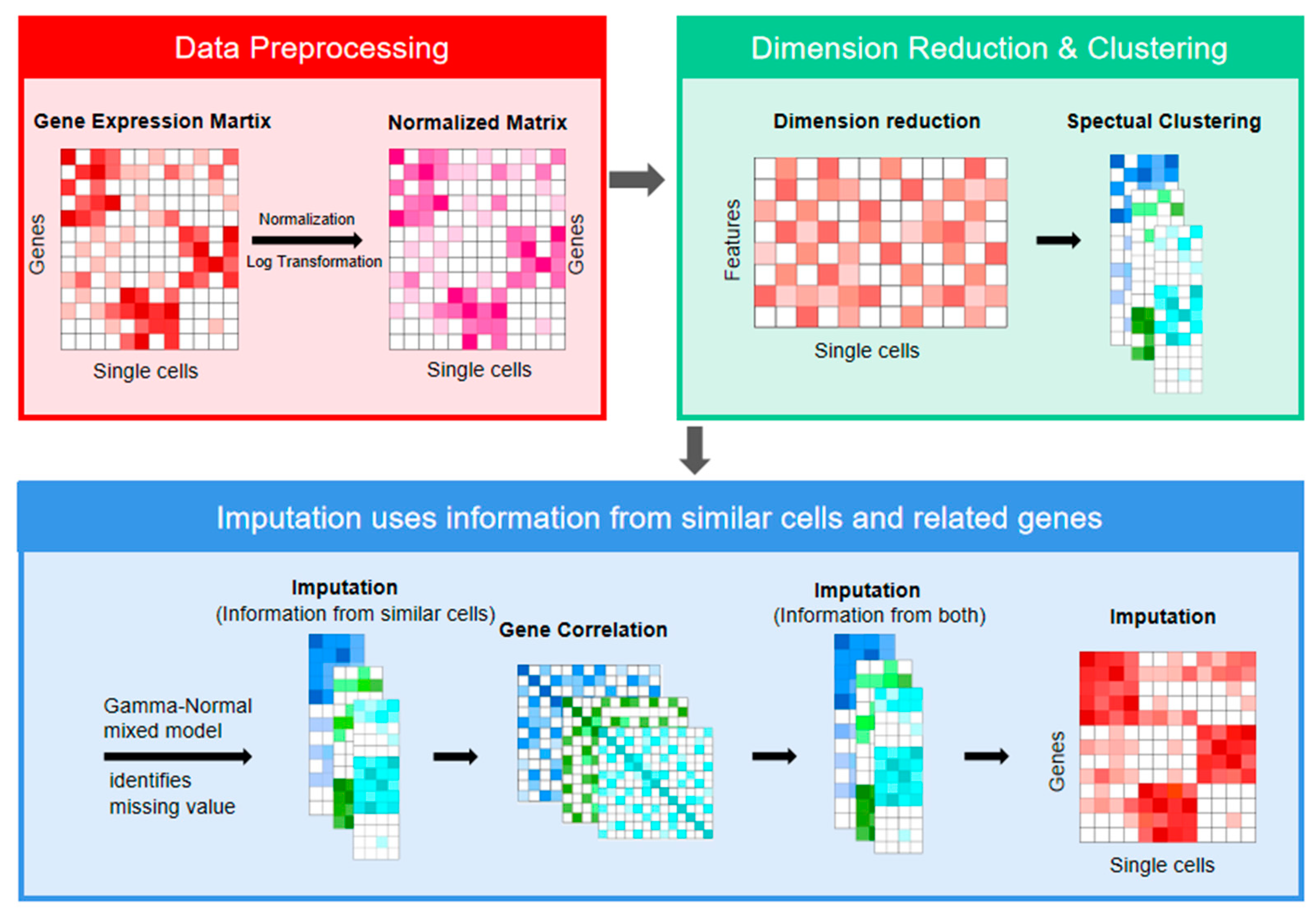
Figure 1. The outline of scCGImpute. scCGImpute takes the scRNA-seq data as input. The output is the imputation that leverages the information between cells and genes simultaneously. The blue, green and cyan colors in the figure represent different cell types. In the matrices, the darkness of colors represents the level of gene expression, while in the gene correlation matrix, the darkness of colors represents the level of correlation.
Applsci 13 07936 g001
Figure 2. For each gene i, random forest was used for regression training on data with high confidence cells (Set A), and then predictions were made for data with low confidence cells (Set B). The set B in the left part is imputed with the information of similar cells, and the set B in the right is the predicted value of the random forest, which is also the final imputation result. The darkness of the color represents the level of gene expression.
Applsci 13 07936 g002
Figure 3. The Results of ARI, NMI, and Purity are shown to evaluate the clustering performance of scCGImpute with other methods on simulated data in line chart form. The value from 0 to 4.5 on the X-axis represents the value of the dropout.mid parameter in splatter, and the percentage in parentheses represents the corresponding dropout rate. The proportion of zero values in reference data is 13.5%.
Applsci 13 07936 g003
Figure 4. The result of Pearson analysis between rawdata and scCGImpute with simulated data. In the figure, refdata represents the correlation between reference data and raw data, and scCGImpute represents the correlation between reference data and scCGImpute. Where “ns” indicates that the p value is greater than 0.05, “**” indicates that the p value is greater than 0.001 and less than or equal to 0.01, and “****” indicates that the p value is less than or equal to 0.0001. (a) Correlation between cells; (b) Correlation between genes.
Applsci 13 07936 g004
Figure 5. The result of Pearson correlation analysis between the imputation and the known concentrations of ERCCs about five sequencing methods. The p value of the t-test for each sequencing data is above the boxplot.
Applsci 13 07936 g005
Figure 6. Stacked graph of three cluster evaluation results (ARI, NMI, and Purity) for four real datasets (Blakeley, Ting, Baron, and Zeisel); (a) Blakeley; (b) Ting; (c) Baron; (d) Zeisel.
Applsci 13 07936 g006
Table 1. The real date sets used in clustering.
DatasetsNumber of Cell TypesNumber of CellsNumber of Genes Cell SourceDropout RateReferences
Blakeley33022,251Human Blastocyst38.2%[34]
Ting718717,251Mouse Pancreatic Circulating Tumor Cells66.7%[35]
Baron14193720,125human pancreatic islets86.9%[36]
Zeisel9300518,378Mouse cortex and hippocampus79.6%[4]
Disclaimer/Publisher’s Note: The statements, opinions and data contained in all publications are solely those of the individual author(s) and contributor(s) and not of MDPI and/or the editor(s). MDPI and/or the editor(s) disclaim responsibility for any injury to people or property resulting from any ideas, methods, instructions or products referred to in the content.