A Three-Way Acceleration Approach for Interval-Valued Multi-Attribute Decision-Making Problems

Abstract

As an essential part of modern intelligent decision-making science, multi-attribute decision-making problems can effectively select and rank all candidate schemes under multiple indicators. Because of the complexity of the real environment and the uncertainty of the decision-making problem, interval numbers are often used to represent the evaluation information of the object. The existing methods of the multi-attribute decision-making problems rarely use the object set but give the decision results by selection or ranking, which often have strong subjectivity. We propose a ranking method from an acceleration viewpoint based on the three-way decision model to solve the interval-valued multi-attribute decision-making problem. A distance measure of two objects is a measure that describes the relationship between objects. Therefore, the fuzzy dominance distance is introduced to express order relations among objects. First, we present a method to compare any two interval numbers, which converts interval numbers into connection numbers according to the characteristics of interval numbers in multi-attribute decision-making problems. Second, the three-way decision theory is introduced to divide the object set into high, medium, and low dominance regions for the speed and rationality of decision-making. Finally, the multi-attribute decision-making problems can be simplified into the problem of selection in three regions by ranking the objects of the selected region. Unlike traditional methods, the experiments demonstrate that our proposed method has the lowest cost. Our method is shown to be efficient and can obtain comparable results.

1. Introduction

Multi-attribute decision-making (MADM) [1,2] is a process based on the objective rule for specific things to achieve a certain goal. With the help of certain tools, techniques, information, and experience, MADM analyzes and calculates many factors affecting the achievement of the goal. We select the best, most satisfactory, and most reasonable method from many possible solutions with the above factors. With people’s in-depth understanding of the MADM problems, we should pay more attention to the influence of the relevance of indicators, the rationality of indicator weighting, and the psychological aspects of decision-makers on this issue. Because of the limitations of cognition about complex things and incomplete data, it is often difficult for people to give evaluation values using certain numbers in actual decision-making. Therefore, how to describe the fuzzy information has become popular [3], and we need to construct an effective method to solve the MADM problems.

1.1. Related Work

The author in [4] proposes a fuzzy set, which has become an important tool for describing fuzzy information and dealing with uncertain problems. Authors in [5] apply neutrosophic similarity measure theory and the distance function to a decision-making model on COVID-19 pandemic patients. Authors in [6] propose a Variable Neighborhood Search (VNS) algorithm based on Multi-Attribute Decision-Making (MADM) strategy under a possibility environment. Under single valued pentapartitioned neutrosophic sets (SVPNS) environment, authors in [7] present a new similarity measure, namely tangent similarity measure, and validate the proposed SVPNS-MADM model. To select an appropriate tender for assigning the work, authors in [8] develop the multi-criteria decision-making model using a single-valued neutrosophic set.

In addition, the basic definitions and properties of the Interval-Valued Intuitionistic Fuzzy Sets (IVIFSs) are presented in [9]. Under the setting of IVIFSs, the authors in [10] propose an optimization model to determine the attribute weights of the MADM problems. The truth degree of an IVIFS is represented by some closed sub-interval of [0, 1] rather than a single value in [0, 1]. Furthermore, the authors in [11] propose the concept of a complex fuzzy set, aiming at the case that the co-domain of a fuzzy set is a set of complex numbers instead of a sub-interval of [0, 1]. Unlike fuzzy numbers, an interval number does not strictly limit the membership degree within [0, 1]. Instead, it is represented by interval, making the meaning more intuitive and accurate. The research on interval numbers can be roughly summarized into two categories, comparison of interval numbers and applications of interval numbers. Interval number comparison means comparing sizes by ordering, and interval-number applications are mainly used in decision-making. The previous studies usually separate these two types of problems, and this paper fills this gap. We not only propose an interval number comparison method but also solve the interval-valued multi-attribute decision-making problem.

As a granular computing method, three-way decision (TWD) theory [12,13,14] deals with many uncertain problems. The author in [15] presents a TWD model employing decision-theoretic rough sets (DTRS). With the help of the Bayesian theory, TWD [16,17] is a methodology that can divide a universal set into three parts with the help of the Bayesian formula. The decision rules are as follows. Positive regions (POS) generate certain rules to decide acceptance, negative regions (NEG) generate certain rules to decide rejection, and boundary regions (BND) decide non-commitment or deferment. The positive and negative regions make strategies for certain objects, and the boundary region makes strategies for uncertain objects [18]. MADM makes a final decision based on many factors that satisfy various demands. Whether it is the MADM or the TWD theory, both provide reasonable methods to choose objects through appropriate criteria [19,20]. Therefore, as the decision-making environment becomes increasingly complex, both are more closely related in decision analysis. The authors in [21] introduced TWD to fuzzy multi-attribute decision-making for the first time and suggested a method to establish the loss function. To better represent the membership and non-membership of the attributes, the authors in [22] construct the TWD model under the intuitionistic fuzzy number. The new model of TWD is proposed in [23], and the decision-making procedure is gained by analyzing Pythagorean fuzzy information systems. The authors in [24] present a novel TWD method to solve the MADM problems in fuzzy information systems. The authors in [25] propose a multi-attribute decision-making method based on the TWD theory in a hesitant fuzzy environment. Based on the above research, exploring the combination of the TWD theory and interval-valued multi-attribute decision-making is possible.

When faced with a choice, people usually do not choose a candidate from just one aspect but will examine many aspects to make a choice. For example, in commuting traffic mode, people will consider not only time but also convenience, comfort, safety, and economy, and other factors and then make a rational choice, which is a typical multi-attribute decision-making problem. As the 4th and 5th industrial revolution advance, authors in [26] use dataspaces to predict the possibility of an employee experiencing attrition with a machine learning predictor. Employee churn (ECn) is a crucial problem for any organization that adversely affects its overall revenue and brand image. To address the problem of employee churn prediction and retention (ECPR), authors in [27] combined multi-attribute decision-making (MADM) with machine learning (ML).

1.2. Contribution

The emergence of the TWD theory offers new opportunities for studying multi-attribute decision-making. Many studies are associated with the TWD theory, such as fuzzy operators, mathematical models with uncertain information, partial order relations based on rough and fuzzy sets, etc. Therefore, using the TWD theory to solve interval-valued multi-attribute decision-making problems is a worthwhile exploration. Different from traditional decision-making methods, this paper combines partition and sorting, that is, by refining the sorting granularity to accelerate the decision-making process. The upper and lower limits of information can be used to express evaluation values by using interval numbers [28], which have gradually become the main trend to express the evaluation of decision-makers [29,30]. Unlike complex q-Rung Orthopair Fuzzy Sets (cq-ROFSs), the interval number controls the membership of an object within a certain range rather than characterizing its non-membership. In practical complex-decision problems, a complex q-rung orthopair fuzzy framework is an effective method to represent fuzzy information, and q-Rung Orthopair Fuzzy Numbers (q-ROFNs) can be aggregated into a single element by using Maclaurin symmetric mean operators [31]. The contributions of this paper are summarized as follows:

• We propose a ranking method based on the distance of fuzzy dominant. By determining the importance of the object through the fuzzy dominance degree and the fuzzy dominance distance, we can make full use of the evaluation value to rank accurately by comparing interval numbers.
• A multi-attribute decision-making acceleration method that combines the TWD theory with the fuzzy dominance distance measurement is put forward. We construct multi-attribute acceleration rules based on the TWD to divide the universal set. Taking “three” as the basic thinking and starting point for solving complex problems is also an innovation.
• According to the decision rules, the MADM problem is simplified to a selection problem in three. We make decisions on finer information blocks (divisions) and provide an effective method for studying MADM.

The methods in [22,32] use intuitionistic fuzzy numbers and fuzzy numbers as attribute values, respectively, and then build loss functions. Compared with traditional MADM methods, we do not directly rank all objects but divide the universal set into three regions. Our method first uses interval numbers as attribute values to construct loss functions. Since a dominance relationship exists among the three regions, we further analyze the decision-making scheme when the needed candidates are determined. Our proposed method is to combine IVMADM and TWD for the first time. Object sets are divided into three regions with a dominance relationship in the fuzzy environment. By contrast, existing MADM methods (TOPSIS, AHP, and VIKOR) directly rank candidates and make the best and worst options.

1.3. Organization

The structure of the paper is organized as follows. Section 2 introduces some definitions. Section 3 discusses the correlation between the interval and connection numbers to get interval fuzzy dominant degrees and presents the TWD theory based on dominance degree. Section 4 explores accelerating rules based on interval fuzzy dominance distance. At the same time, the ranking method is discussed from different regions. Section 5 gives a practical example of the proposed MADM methods based on the TWD theory. We conclude the paper in Section 6.

2. Preliminary Knowledge

This section will examine some knowledge, including basic concepts, definitions, and operations of interval and connection numbers.

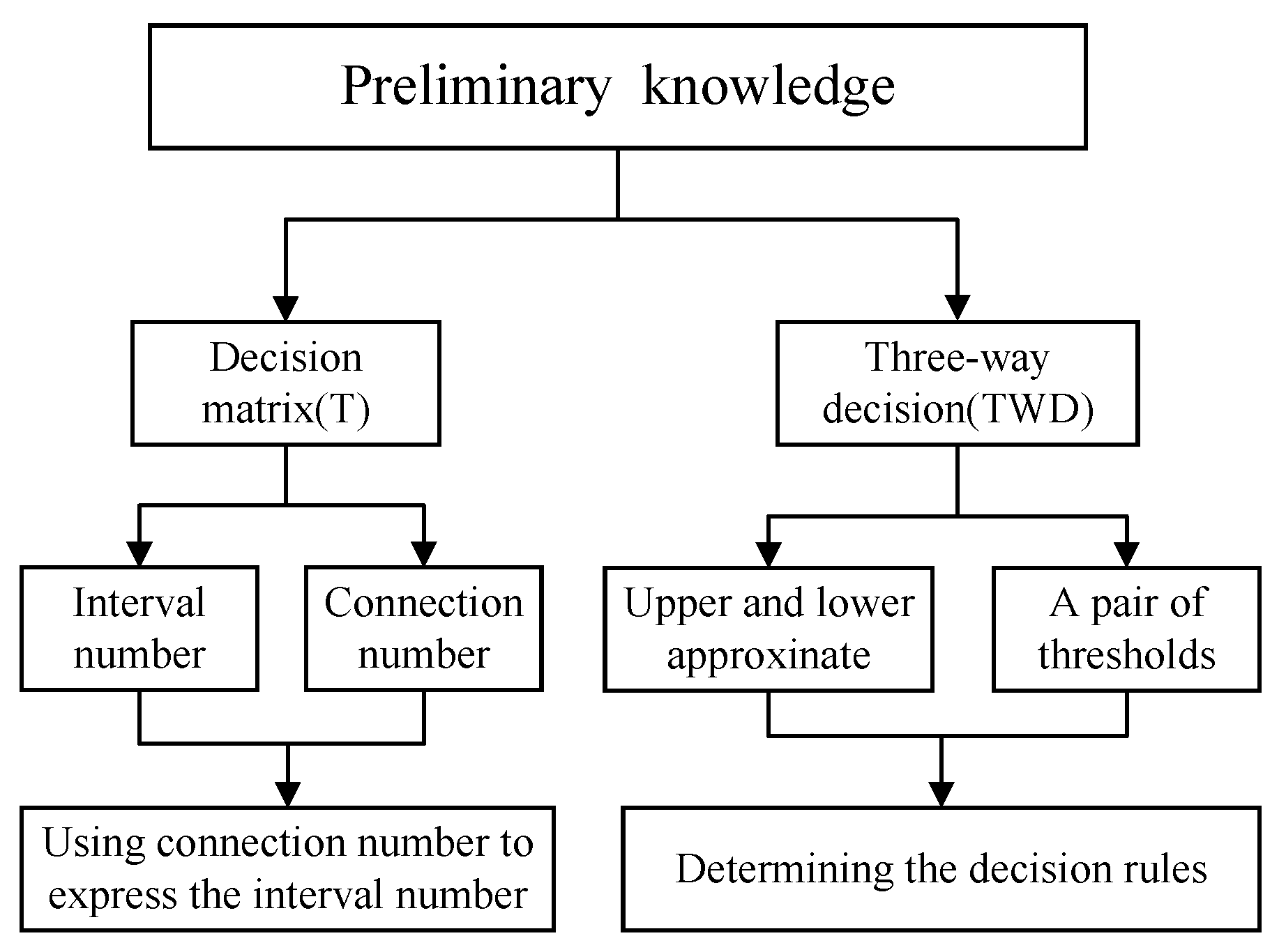
Since the paper mainly uses TWD theory to solve the interval-valued multi-attribute decision-making problem, the following content introduces the knowledge related to interval numbers and TWD theory. The structure of this section is shown in Figure 1.

2.1. Problem Description

We take an interval-valued decision matrix as the research object and introduce the relationship between interval number and connection number to compare interval numbers better.

$U=\{x_1,x_2,\dots ,x_m\}$ represents the candidates, and $K=\{k_1,k_2,\dots ,k_n\}$ represents attribute collection, which describes the characteristics of each candidate. $\mathsf{\Omega }=\{{\omega }_{k_1},{\omega }_{k_2},\dots ,{\omega }_{k_n}\}$ represents attribute weight, corresponding to K. Note that $0<{\omega }_{k_p}<1$ and ${\displaystyle \sum _{p=1}^n}{\omega }_{k_p}=1$. $T=t_{q{k}_p}$ represents the decision matrix. $1\le q\le m$, $1\le p\le n$, $t_{q{k}_p}$ is the evaluation information of candidate q under the $k_p$.

There are many ways to describe the uncertainty of things; compared with other methods, the advantage of the interval number is used to express the information by upper and lower limits. Therefore, the interval-valued (IV) information system can be defined as $f(x_i,k_p)=[a_i^l,a_i^u]$, 1$\le i\le$ m, 1 $\le p\le$n.

Set pair analysis is widely used in interval number multi-attribute decision-making because the connection number has both deterministic and uncertain properties. This is similar to interval number characteristics, which have both the certainty of upper and lower bounds and the uncertainty of arbitrary values in their range. The connection number is a method to deal with uncertain information. The core idea is to deal with the comprehensive problem of uncertainty systematically by analyzing objective things’ certainty and uncertainty measures from the three aspects of the same degree, difference degree, and opposition degree of objects. It can be described as

$$\begin{array}{cc}\hfill \mu \left(W\right)& ={\displaystyle \frac{H}{M}}+{\displaystyle \frac{F}{M}}e+{\displaystyle \frac{T}{M}}g\hfill \\ \hfill & =a+be+cg,\hfill \end{array}$$

(1)

where $e\in [-1,1]$, $g\in [-1,1]$. a, b, c meet the normalization conditions: $a+b+c=1$. Assuming that there are two sets, we analyze the characteristics of set A and set B under the problem W. ${\displaystyle \frac{H}{M}}$ represents the common characteristics of set A and set B under the problem W, i.e., the same degree, denoting a. ${\displaystyle \frac{F}{M}}$ represents the opposite characteristics of set A and set B under the problem W, namely the difference degree or uncertainty, denoted as b. ${\displaystyle \frac{T}{M}}$ represents the differential characteristics of set A and set B under the problem W, namely, the degree of opposition, denoted by c. Therefore, $\mu \left(W\right)$ can be simplified to $a+be$.

From the perspective of mathematical analysis, the uncertainty of the value of the connection number is mainly reflected in the difference of the uncertain coefficient e in the given interval [−1, 1], which makes any interval number to be easily converted into a connection number so that it is possible to establish a decision model based on this basis. e varies according to specific problems. Therefore, e has no practical significance when comparing interval numbers. An interval number [33] $A=[a^l,a^u]$=$\{a^l<x<a^u,a^l,x\in R\}$ is expressed as

$$A=[{\lambda }_1\left(A\right),{\lambda }_2\left(A\right)],$$

(2)

where ${\lambda }_1\left(A\right)$=${\displaystyle \frac{a^l+a^u}{2}}$ represents the expected value of A and reflects the size of A. ${\lambda }_2\left(A\right)$ = ${\displaystyle \frac{a^u-a^l}{2}}$ reflects the uncertain degree of A. A can be expressed as $A={\displaystyle \frac{a^l+a^u}{2}}+{\displaystyle \frac{a^u-a^l}{2}}e$. e is the regulatory factor, which is different in $\mu \left(W\right)$ and A. Using the connection number to express the interval number can more clearly reflect the characteristics of the interval number.

2.2. Three-Way Decision Theory

Three-way decision (TWD) is an influential theory of study knowledge discovery and intelligence data decision. We mainly use the decision rules in TWD theory to divide decision objects and then compare them. A central notion of the TWD [34,35] is to transform a whole into and apply corresponding actions into three parts. The idea is commonly used in the actual human decision-making processes [36,37,38]. Therefore, the mathematical model of the three-way rough set (RS) is presented.

Definition 1.

U is called a non-empty finite object set, $\tilde{R}$ is named an equivalence relation on U. An approximation space is expressed by $apr=(U,\tilde{R})$, $U/\tilde{R}=\left\{\left[x\right]\right|x\in U\}$. For $\tilde{C}\subseteq U$, the upper and lower approximate sets of $\tilde{C}$ are outlined as:

$$\begin{array}{ccc}\hfill \underline{apr}\left(\tilde{C}\right)& =& \{x\in U|\left[x\right]\subseteq \tilde{C}\},\hfill \\ \hfill \overline{apr}\left(\tilde{C}\right)& =& \{x\in U|\left[x\right]\cap \tilde{C}\ne \varnothing \}.\hfill \end{array}$$

(3)

Definition 2.

Let $Pr\left(\tilde{C}\right|\left[x\right])$ denote the conditional probability. The pair $ap{r}_{(\alpha ,\beta )}=(U,\tilde{R})$ denote an $(\alpha ,\beta )$-probabilistic approximation space. For $\tilde{C}\subseteq U$, the $(\alpha ,\beta )$-probabilistic approximations are provided by $POS{\left(\tilde{C}\right)}_{(\alpha ,\beta )}$, $BND{\left(\tilde{C}\right)}_{(\alpha ,\beta )}$ and $NEG{\left(\tilde{C}\right)}_{(\alpha ,\beta )}$:

$$\begin{array}{ccc}\hfill POS{\left(\tilde{C}\right)}_{(\alpha ,\beta )}& =& \{x\in U|Pr\left(\tilde{C}\right|\left[x\right])⩾\alpha \},\hfill \\ \hfill BND{\left(\tilde{C}\right)}_{(\alpha ,\beta )}& =& \{x\in U|\beta <Pr\left(\tilde{C}\right|\left[x\right])<\alpha \},\hfill \\ \hfill NEG{\left(\tilde{C}\right)}_{(\alpha ,\beta )}& =& \{x\in U|Pr\left(\tilde{C}\right|\left[x\right])⩽\beta \}.\hfill \end{array}$$

(4)

When a pair of approximate is introduced into the whole set U, the U becomes three independent regions. Moreover, the authors [39] proposed a decision-theoretic rough set (DTRS), which explains three-way rules based on Bayesian theory.

We use $\mathsf{\Omega }=\{\tilde{C},\neg \tilde{C}\}$ represents two states in the set and $\mathsf{\Gamma }=\{a_P,a_B,a_N\}$ represents three actions in the set [39]. $a_P$, $a_N$, and $a_B$ represent $x\in POS\left(\tilde{C}\right)$, $x\in NEG\left(\tilde{C}\right)$ and $x\in BND\left(\tilde{C}\right)$, respectively. Meanwhile, there are six parameters describing the loss functions. ${\dot{\upsilon }}_{PP}$, ${\dot{\upsilon }}_{BP}$, and ${\dot{\upsilon }}_{NP}$ represent the loss when x belongs to $\tilde{C}$ and takes actions $a_P$, $a_B$, and $a_N$, respectively. Similarly, ${\dot{\upsilon }}_{PN}$, ${\dot{\upsilon }}_{BN}$, and ${\dot{\upsilon }}_{NN}$ represent the loss when x belongs to $\neg \tilde{C}$ and takes action $a_P$, $a_B$, and $a_N$, respectively. Furthermore, the loss function meets the conditions ${\dot{\upsilon }}_{PP}⩽{\dot{\upsilon }}_{BP}<{\dot{\upsilon }}_{NP}$ and ${\dot{\upsilon }}_{PN}⩽{\dot{\upsilon }}_{BN}<{\dot{\upsilon }}_{NN}$.

The expected loss under different actions can be shown as follows:

$$\begin{array}{cc}\hfill {\tilde{\varrho }}_{a_P}& ={\dot{\upsilon }}_{PP}Pr(\tilde{C}\mid \left[x\right])+{\dot{\upsilon }}_{PN}Pr(\neg \tilde{C}\mid \left[x\right]),\hfill \\ \hfill {\tilde{\varrho }}_{a_B}& ={\dot{\upsilon }}_{BP}Pr(\tilde{C}\mid \left[x\right])+{\dot{\upsilon }}_{BN}Pr(\neg \tilde{C}\mid \left[x\right]),\hfill \\ \hfill {\tilde{\varrho }}_{a_N}& ={\dot{\upsilon }}_{NP}Pr(\tilde{C}\mid \left[x\right])+{\dot{\upsilon }}_{NN}Pr(\neg \tilde{C}\mid \left[x\right]).\hfill \end{array}$$

(5)

Based on the risk minimization process, if Min(${\varrho }_{a_P}$,${\varrho }_{a_B}$,${\varrho }_{a_N}$ ) = ${\varrho }_{a_P}$, the object x belongs to $POS\left(\tilde{C}\right)$; if Min(${\varrho }_{a_P}$,${\varrho }_{a_B}$,${\varrho }_{a_N}$) = ${\varrho }_{a_B}$, the object x belongs to $BNG\left(\tilde{C}\right)$; if Min(${\varrho }_{a_P}$,${\varrho }_{a_B}$,${\varrho }_{a_N}$) = ${\varrho }_{a_N}$, the object x belongs to $NEG\left(\tilde{C}\right)$.

Since $Pr(\tilde{C}\mid \left[x\right])$ + $Pr(\neg \tilde{C}\mid \left[x\right])$ = 1, the above rules can be transformed into the relationship between $Pr(\tilde{C}\mid \left[x\right])$ and $\alpha$ and $\beta$.

A pair of thresholds $(\alpha ,\beta )$ in the range of $0\le \beta <\alpha \le 1$ by minimizes $\tilde{\varrho }$ is obtained as:

$$\begin{array}{c}\hfill \alpha ={\displaystyle \frac{({\dot{\upsilon }}_{PN}-{\dot{\upsilon }}_{BN})}{({\dot{\upsilon }}_{PN}-{\dot{\upsilon }}_{BN})+({\dot{\upsilon }}_{BP}-{\dot{\upsilon }}_{PP})}},\\ \hfill \beta ={\displaystyle \frac{({\dot{\upsilon }}_{BN}-{\dot{\upsilon }}_{NN})}{({\upsilon }_{BN}-{\upsilon }_{NN})+({\dot{\upsilon }}_{NP}-{\dot{\upsilon }}_{BP})}}.\end{array}$$

The risk functions with the minimum-cost criterion can systematically calculate $\alpha$ and $\beta$. In brief, the decision rules are determined by conditional probability and the threshold.

3. TWD Model with Degree Measure

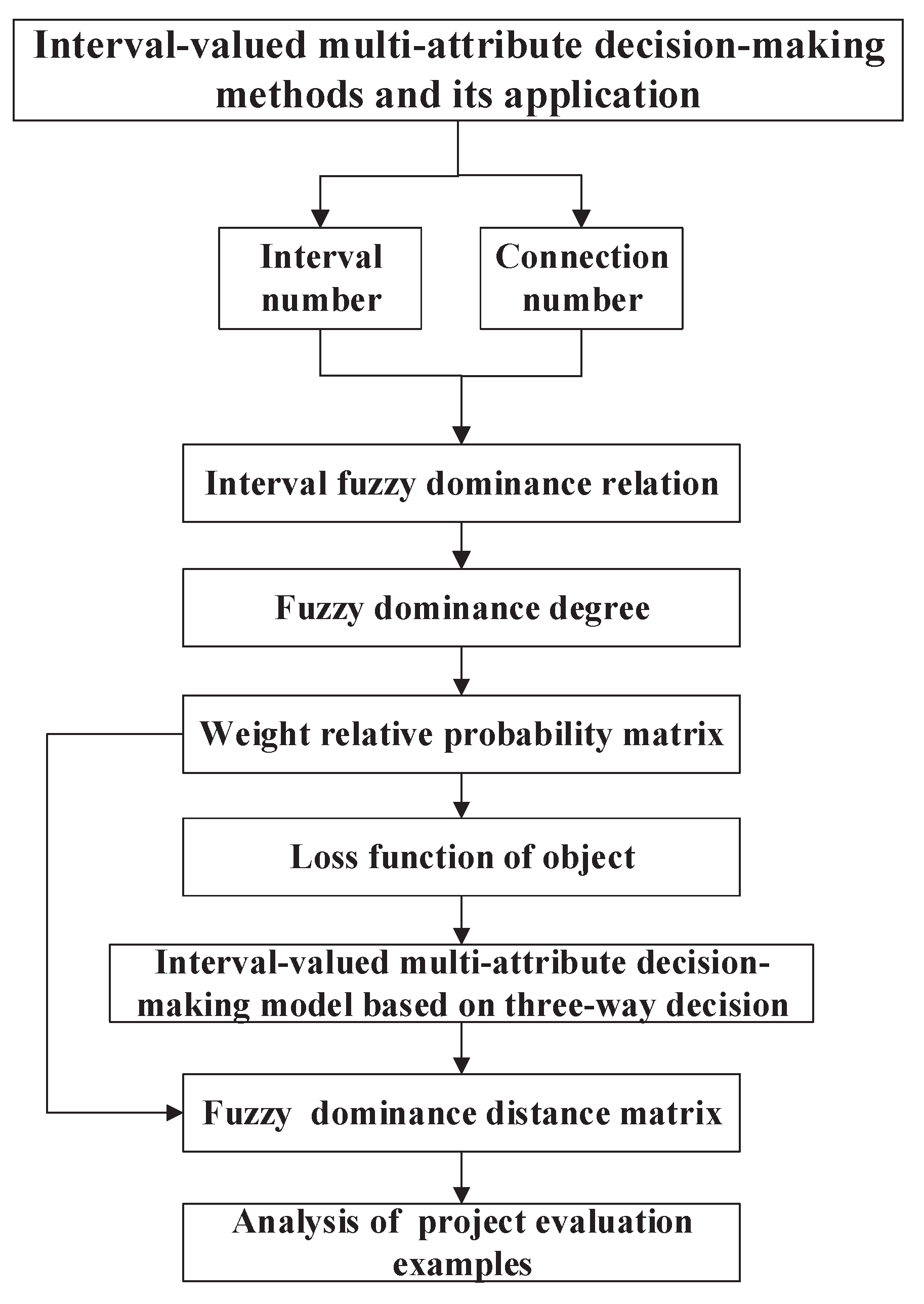
In this section, we pay more attention to the TWD of IVIS. The specific representation of the interval number is given to compute the dominance degree; then, we construct a new method of the loss function in TWD. Figure 2 describes the workflow of this article.

3.1. Interval Fuzzy Dominance Relationship

This section proposes the concepts of intersecting and non-intersecting interval numbers. We use connection numbers to express the corresponding interval numbers and then establish decision models to compare any two interval numbers.

Definition 3.

Let $y_i=[a_i^l,a_i^u],y_j=[a_j^l,a_j^u]$ be any two interval numbers. The comparison between $y_i=[a_i^l,a_i^u]$ and $y_j=[a_j^l,a_j^u]$ is presented as follows:

1. 

If $a_i^l<a_j^l<a_i^u<a_j^u$, $y_i$ and $y_j$ are called the intersecting interval numbers;

2. 

If $(a_i^u<a_j^l)\vee (a_j^u<a_i^l)$, $y_j$ and $y_j$ are called the non-intersecting interval numbers;

3. 

$a_j^l<a_i^l<a_i^u<a_j^u$ or $a_i^l<a_j^l<a_j^u<a_i^u$, they are special examples of intersecting interval numbers.

Here, $e\in [-1,1]$, and it reflects uncertainty of the connection number.

Definition 4.

Suppose that $y_i=[a_i^l,a_i^u]$ and $y_j=[a_j^l,a_j^u]$ are any intersecting interval numbers. $y_i$ and $y_j$ can be defined in the following

$$\begin{array}{c}\hfill y_i^{\prime }={\displaystyle \frac{a_i^l+a_i^u}{2}}+{\displaystyle \frac{a_i^u-a_j^l}{a_i^u-a_i^l}}e,\\ \hfill y_j^{\prime }={\displaystyle \frac{a_j^l+a_j^u}{2}}+{\displaystyle \frac{a_i^u-a_j^l}{a_j^u-a_j^l}}e,\end{array}$$

(6)

where ${\displaystyle \frac{a_i^l+a_i^u}{2}}$ and ${\displaystyle \frac{a_j^l+a_j^u}{2}}$ represent the midpoints of $y_i$ and $y_j$, respectively. ${\displaystyle \frac{a_i^u-a_j^l}{a_i^u-a_i^l}}$ and ${\displaystyle \frac{a_i^u-a_j^l}{a_j^u-a_j^l}}$ represent the proportion of the determined distances on $y_i$ and $y_j$, respectively. $y_i^{\prime }$ and $y_j^{\prime }$ represent the connection numbers derived from $y_i$ and $y_j$, respectively.

We can interpret that the new $y_i$ is composed of two parts, one is the midpoint of a certain interval number, and another is an uncertain measurement of the intersecting part in the previous $y_i$. Since it is difficult to compare any intersecting interval numbers $y_i$ and $y_j$, they are first represented by the connection number and then compared. In particular, when comparing the interval number $y_i=[a_i^l,a_i^u]$ and $y_j=[a_j^l,a_j^u]$, we have $y_j>y_i$ if, and only if, $a_j^l<a_i^l<a_i^u<a_j^u$.

Definition 5.

Let $a+be$ be a connection number. Based on the principle of connection number plural operation, the modulus of $a+be$ is given by

$$\begin{array}{c}\hfill r=\sqrt{a^2+b^2},\end{array}$$

(7)

where $r=\sqrt{a^2+b^2}$ is an interval multi-attribute decision vector projection model based on the connection number whose type is $a+be$.

According to Definition 5, we may quickly obtain the decision vector projection model of the interval number and compare any two-interval-number. The comparison model is as follows:

1.

$y_i=[a_i^l,a_i^u]$ and $y_j=[a_j^l,a_j^u]$ are any two intersecting interval numbers and the decision vector projection models of $y_i$, and $y_j$ are:

$$\begin{array}{cc}\hfill r_i& =\sqrt{{\left({\displaystyle \frac{a_i^l+a_i^u}{2}}\right)}^2+{\left({\displaystyle \frac{a_i^u-a_j^l}{a_i^u-a_i^l}}\right)}^2},\hfill \\ \hfill r_j& =\sqrt{{\left({\displaystyle \frac{a_j^l+a_j^u}{2}}\right)}^2+{\left({\displaystyle \frac{a_i^u-a_j^l}{a_j^u-a_j^l}}\right)}^2},\hfill \end{array}$$

(8)

if $r_i>r_j$, then $y_i\succcurlyeq y_j$, else then $y_i\prec y_j.$

2.

$y_i=[a_i^l,a_i^u]$ and $y_j=[a_j^l,a_j^u]$ are any two non-intersecting interval numbers, which can be expressed and compared according to Definitions 4 and 5.

Definition 6.

Let $S=(U,AT,V,f)$ be an interval-valued information system [40,41]. Under the same attribute, we use the interval fuzzy dominance probability to express the relative degree between objects. The interval fuzzy dominance probability is $x_{ij}$.

Therefore, we define T as an interval-valued decision matrix mentioned above.

$$T=\left[\begin{array}{cccc}[a_{1k_1}^l,a_{1k_1}^u]& [a_{1k_2}^l,a_{1k_2}^u]& \cdots & [a_{1k_n}^l,a_{1k_n}^u]\\ [a_{2k_1}^l,a_{2k_1}^u]& [a_{2k_2}^l,a_{2k_2}^u]& \cdots & [a_{2k_n}^l,a_{2k_n}^u]\\ ⋮& ⋮& [a_{i{k}_p}^l,a_{i{k}_p}^u]& ⋮\\ [a_{m{k}_1}^l,a_{m{k}_1}^u]& [a_{m{k}_2}^l,a_{m{k}_2}^u]& \cdots & [a_{m{k}_n}^l,a_{m{k}_n}^u]\end{array}\right].$$

For $x_i\in U$, attributes $k_p\in AT$, $1\le i⩽m$, $1\le p⩽n$, of the evaluation value of the ith alternatives are denoted by $a_{ikp}$. Thus, $a_{i{k}_p}=f(x_i,k_p)=[a_{i{k}_p}^l,a_{i{k}_p}^u]$. That is, $k_p\in K$, the corresponding fuzzy dominance probability matrix is denoted by $X_{k_p}=\left(x_{ij}^{k_p}\right)$, and $x_{ij}^{k_p}$ denotes the degree of $x_i$ superior to $x_j$ under the attribute $k_p$. According to the actual situation, there are two ways to build $x_{ij}^{k_p}$:

• If $\sim {\left[f(x_i,k_p)\right]}^{\succcurlyeq }\cup {\left[f(x_j,k_p)\right]}^{\succcurlyeq }=U$, the dominance degree of $x_i$ superior to $x_j$ is:

  $$x_{ij}={\displaystyle \frac{\left|U\right|}{\left|U\right|+|{\left[f(x_i,k_p)\right]}^{\succcurlyeq }\bigcup \sim {\left[f(x_j,k_p)\right]}^{\succcurlyeq }|}}.$$

  (9)
• If $\sim {\left[f(x_i,k_p)\right]}^{\succcurlyeq }\bigcup {\left[f(x_j,k_p)\right]}^{\succcurlyeq }\ne U$, the dominance degree of $x_i$ superior to $x_j$ is:

  $$x_{ij}={\displaystyle \frac{|\sim {\left[f(x_i,k_p)\right]}^{\succcurlyeq }\bigcup {\left[f(x_j,k_p)\right]}^{\succcurlyeq }|}{\left|U\right|+|\sim {\left[f(x_i,k_p)\right]}^{\succcurlyeq }\bigcup {\left[f(x_j,k_p)\right]}^{\succcurlyeq }|}}.$$

  (10)

Here, ${\left[f(x_i,k_p)\right]}^{\succcurlyeq }$ denotes the dominance class of $x_i$ under attribute $k_p$, $\sim {\left[f(x_j,k_p)\right]}^{\succcurlyeq }$ denotes the non-dominance class of $x_j$ under attribute $k_p$.

The matrix composed of $x_{ij}$ is called an interval fuzzy dominance probability matrix, which is denoted as $X_{k_p}$. According to the Definition 6, the fuzzy dominance probability matrix $\stackrel{\sim }{X_{k_p}}$ is as follows:

$$\stackrel{\sim }{X_{k_p}}=\left[\begin{array}{cccc}{x}_{11}^{k_p}& x_{12}^{k_p}& \cdots & x_{1m}^{k_p}\\ x_{21}^{k_p}& x_{22}^{k_p}& \cdots & x_{2m}^{k_p}\\ ⋮& ⋮& x_{ij}^{k_p}& ⋮\\ x_{m1}^{k_p}& x_{m2}^{k_p}& \cdots & x_{mm}^{k_p}\end{array}\right].$$

Definition 7.

Given that $S=(U,AT,V,f)$ and $x_i$ and $x_j$ are any two objects under same attributes, $R_B^{\succcurlyeq }$ and $R_B^{\prec }$ can be described separately in the following

$$\begin{array}{c}\hfill \begin{array}{cc}\hfill R^{\succcurlyeq }& =\{(x_i,x_j)\in U^2\mid f(k_p,x_i)⩾f(k_p,x_j)(k_p\in K)\},\hfill \\ \hfill R^{\prec }& =\{(x_i,x_j)\in U^2\mid f(k_p,x_i)<f(k_p,x_j)(k_p\in K)\},\hfill \end{array}\end{array}$$

(11)

where $R^{\succcurlyeq }$ and $R^{\prec }$ are called dominating and dominated relationships, respectively, and also $f(k_p,x_i)\ge f(k_p,x_j)\iff [a_{i{k}_p}^l,a_{i{k}_p}^u]\ge [a_{j{k}_p}^l,a_{j{k}_p}^u]$($k_p$∈K).

3.2. TWD Based on Dominance Degree

In the previous subsection, we establish a TWD model for the MADM problems whose attributes are exact and intuitionistic fuzzy numbers. This subsection will explore a TWD model to handle the MADM problems. We introduce a method to compute the relative loss function between attribute values and the loss function. The relative loss functions are introduced as follows:

Table 1. The relative loss functions.

	$\tilde{\mathit{C}}$	$\neg \tilde{\mathit{C}}$
$a_P$	0	${\ddot{\upsilon }}_{PN}$
$a_B$	${\ddot{\upsilon }}_{BP}$	${\ddot{\upsilon }}_{BN}$
$a_N$	${\ddot{\upsilon }}_{NP}$	0

shows the relative loss functions in two states, where ${\ddot{\upsilon }}_{PN}={\dot{\upsilon }}_{PN}-{\dot{\upsilon }}_{NN}$, ${\ddot{\upsilon }}_{BN}={\dot{\upsilon }}_{BN}-{\dot{\upsilon }}_{NN}$, ${\ddot{\upsilon }}_{BP}={\dot{\upsilon }}_{BP}-{\dot{\upsilon }}_{PP}$, and ${\ddot{\upsilon }}_{NP}={\dot{\upsilon }}_{NP}-{\dot{\upsilon }}_{PP}$. The significance of the relative loss function can be expressed as if an object belongs to $\neg \tilde{C}$, the relative losses of $a_P,a_B,a_N$ can be denoted by ${\ddot{\upsilon }}_{PN}$, ${\ddot{\upsilon }}_{BN}$, and 0, respectively; if an object belongs to $\neg \tilde{C}$, the relative losses of $a_P,a_B,a_N$ to $a_N$ can be denoted by ${\ddot{\upsilon }}_{PN}$, ${\ddot{\upsilon }}_{BN}$, and 0, respectively.

Based on the relative loss functions in two states,

Table 2. The IV’s loss functions.

	$\tilde{\mathit{C}}$	$\neg \tilde{\mathit{C}}$
$a_P$	0	$x_{max}^j-x_{ij}$
$a_B$	$\psi (x_{ij}-x_{min}^j)$	$\psi (x_{max}^j-x_{ij})$
$a_N$	$x_{ij}-x_{min}^j$	0

shows the relative loss functions of interval numbers, where $x_{max}^j$ = $Max(x_{i1},x_{i2},\cdots ,x_{im})$, $x_{min}^j$ = $Min(x_{i1},x_{i2},\cdots ,x_{im})$, $i\in (1,m)$. In Table 2, $x_{ij}-x_{min}^j,$ indicates the superiority of the object $x_i$ over $x_j$ when decision-makers reject the objects $x_i$ belonging to $\tilde{C}$. $x_{max}^j-x_{ij}$ represents the deficiency of $x_i$ to $x_j$ when decision-makers accept the objects $x_i$ belonging to $\neg \tilde{C}$. According to the TWD theory, thresholds are calculated as follows:

$$\begin{array}{cc}\hfill & {\alpha }^{\prime }={\displaystyle \frac{(1-\psi )(x_{max}^j-x_{ij})}{\left((1-\psi )(x_{max}^j-x_{ij})\right)+\psi (x_{ij}-x_{min}^j)}},\hfill \\ \hfill & {\beta }^{\prime }={\displaystyle \frac{\psi (x_{max}^j-x_{ij})}{\psi (x_{max}^j-x_{ij})+(1-\psi )(x_{ij}-x_{min}^j)}},\hfill \\ \hfill & {\gamma }^{\prime }={\displaystyle \frac{x_{max}^j-x_{ij}}{x_{max}^j-x_{min}^j}}.\hfill \end{array}$$

(12)

U is a set which is made up of $\{x_1,x_2,\cdots ,x_m\}$, $AT$ is composed of $\{k_1,k_2,\cdots ,k_n\}$, and $\omega =\{{\omega }_{k_1},{\omega }_{k_2},\cdots ,{\omega }_{k_n}\}$ is a set of attributes weight where $\omega \in (0,1)$. All fuzzy dominance probability matrixes are aggregated to form the weight-relative probability matrix. It is defined as $D\left(\stackrel{\sim }{B}\right)$:

$$D\left(\stackrel{\sim }{B}\right)=\left[\begin{array}{ccc}{w}_{k_1}{x}_{11}^{k_1}+\cdots +w_{k_n}{x}_{11}^{k_n},& \cdots ,& w_{p_1}{x}_{1m}^{k_1}+\cdots +w_{k_n}{x}_{1m}^{k_n}\\ ⋮& & ⋮\\ w_{k_1}{x}_{m1}^{k_1}+\cdots +w_{k_n}{x}_{m1}^{k_n}& ,\cdots ,& w_{k_1}{x}_{mm}^{k_1}+\cdots +w_{k_n}{x}_{mm}^{k_n}\end{array}\right].$$

(13)

The weight-relative probability matrix can be expressed as follows:

$$D\left(\stackrel{\sim }{B}\right)=\left[\begin{array}{cccc}{b}_{11}& b_{12}& \cdots & b_{1m}\\ b_{21}& b_{22}& \cdots & b_{2m}\\ ⋮& ⋮& b_{ij}& ⋮\\ b_{m1}& b_{m2}& \cdots & b_{mm}\end{array}\right].$$

By converting each row of the weight-relative probability matrix, we can get the degree that each element is superior to other objects as follows:

$$b_{average}={\displaystyle \frac{{\displaystyle \sum _{j=1}^m}{b}_{ij}}{m}}.$$

(14)

Suppose that the evaluation value is an interval number. $\mathsf{\Omega }$ = $\{\tilde{C},\neg \tilde{C}\}$ indicates that an object is better or worse than others. According to Table 2, the relative loss function under each attribute can be obtained.

In

Table 3. The IV’s relative loss functions.

	$\tilde{\mathit{C}}$	$\neg \tilde{\mathit{C}}$
$a_P$	0	$b_{·j\left(max\right)}-b_{·j\left(average\right)}$
$a_B$	$\psi (b_{·j\left(average\right)}-b_{·j\left(min\right)})$	$\psi (b_{·j\left(max\right)}-b_{·j\left(average\right)})$
$a_N$	$b_{·j\left(average\right)}-b_{·j\left(min\right)}$	0

, ${\ddot{\upsilon }}_{PP}$ = 0 and ${\ddot{\upsilon }}_{NN}$ = 0 indicate that the cost of misclassification is minimized, where $b_{·j\left(max\right)}=Max(b_{i1},b_{i2},\cdots ,b_{im})$ and $b_{·j\left(min\right)}=Min(b_{i1},b_{i2},\cdots ,b_{im})$, $i\in (1,m)$. $b_{·j\left(max\right)}$ represents the max degree that the object is superior to other objects, and $b_{·j\left(min\right)}$ represents the minimum degree that the object is inferior to other objects. When $x_i\in \tilde{C}$, the cost of misclassification is 0, the maximum loss of misclassification is ${\ddot{\upsilon }}_{NP}$ and is denoted as $b_{·j\left(average\right)}-b_{·j\left(min\right)}$. Similarly, we can prove that $x_i\in \neg \tilde{C}$.

According to the method of the loss function and Table 3, thresholds can be denoted as:

$$\begin{array}{cc}\hfill & {\tilde{\alpha }}^{\prime }={\displaystyle \frac{(1-\psi )(b_{·j\left(max\right)}-b_{·j\left(average\right)})}{\left((1-\psi )(b_{·j\left(max\right)}-b_{·j\left(average\right)})\right)+\psi (b_{·j\left(average\right)}-b_{·j\left(min\right)})}},\hfill \\ \hfill & {\tilde{\beta }}^{\prime }={\displaystyle \frac{\psi (s_{·j\left(max\right)}-s_{·j\left(average\right)})}{\left(\psi (b_{·j\left(max\right)}-b_{·j\left(average\right)})\right)+(1-\psi )(b_{·j\left(average\right)}-b_{·j\left(min\right)})}},\hfill \\ \hfill & {\tilde{\gamma }}^{\prime }={\displaystyle \frac{b_{·j\left(max\right)}-b_{·j\left(average\right)}}{b_{·j\left(max\right)}-b_{·j\left(min\right)}}}.\hfill \end{array}$$

(15)

We can conclude that ${\tilde{\alpha }}^{\prime }$ and ${\tilde{\beta }}^{\prime }$ are affected by $b_{·j\left(max\right)}$, $b_{·j\left(min\right)}$ and $b_{·j\left(average\right)}$ and $\psi$, ${\tilde{\gamma }}^{\prime }$ is affected by $b_{·j\left(max\right)}$,$b_{·j\left(min\right)}$ and $b_{·j\left(average\right)}$.

When $\psi =0$, we obtain ${\tilde{\alpha }}^{\prime }=1$ and ${\tilde{\beta }}^{\prime }=0$, which means that all objects are grouped into regions of non-commitment; when $0<{\psi }^{\prime }<0.5$, the thresholds meet the condition of the TWD; when $\psi =0.5$, we obtain ${\tilde{\alpha }}^{\prime }={\tilde{\gamma }}^{\prime }={\tilde{\beta }}^{\prime }$, and no object is assigned to the region of non-commitment. When $0.5<\psi <1$, the problem is still simplified as a two-way decision model satisfying $0<{\tilde{\alpha }}^{\prime }<{\tilde{\gamma }}^{\prime }<{\tilde{\beta }}^{\prime }<1$; the two-way decisions are only influenced by $\psi$ when ${\tilde{\alpha }}^{\prime }=0$ and ${\tilde{\beta }}^{\prime }=1$.

When $\psi =0$, ${\tilde{\alpha }}^{\prime }=1$, and ${\tilde{\beta }}^{\prime }=0$, there is only boundary region. When the parameter $\psi$ ranges from 0 to 1, we can get the following decision rules:

$$\begin{array}{cc}\hfill \left(P_2\right)& ifPr(\tilde{C}\mid \left[x_i\right])\ge {\tilde{\alpha }}^{\prime },then{x}_i\in POS\left(\tilde{C}\right),\hfill \\ \hfill \left(B_2\right)& if\tilde{\alpha }>Pr(\tilde{C}\mid \left[x_i\right])>{\tilde{\beta }}^{\prime },then{x}_i\in BND\left(\tilde{C}\right),\hfill \\ \hfill \left(N_2\right)& ifPr(\tilde{C}\mid \left[x_i\right])\le {\tilde{\beta }}^{\prime },then{x}_i\in NEG\left(\tilde{C}\right).\hfill \end{array}$$

(16)

4. Interval-Valued Multi-Attribute Decision-Making (IVMADM) Model Based on TWD

We first present the division rules based on the TWD theory in the IVMADM problems to obtain three regions and propose ranking objects in specific regions.

4.1. Acceleration Rules Based on TWD

According to traditional MADM methods, all the objects are sorted in a certain way (i.e., an object is decided to be accepted or rejected), and then the optimal object is selected. In contrast, those approaches ignore the need in many real applications because the decision-making result is harsh. For example, the decision process can be complicated in the campus recruitment problem, as the number of candidates needed is known. If all candidates are ranked, the decision process is complex and produces redundant results for decision-makers. To overcome the limitations mentioned above, we use the TWD theory to divide U into three regions, from which alternatives can be determined given the number of candidates needed. These three regions are high dominance regions, medium dominance regions, and low dominance regions, and their dominance relationship decreases one by one.

We analyze the MADM problems under the situation that there is a set U of m candidates, and its subset $U_1$ with the size of $m_1$ should be selected. According to the TWD theory, U can be divided into positive region ($POS\left(\tilde{C}\right)$), boundary region ($BND\left(\tilde{C}\right)$), and negative region ($NEG\left(\tilde{C}\right)$), with the size of $M_1$, $M_2$, and $m-M_1-M_2$, respectively. Under the conditions of different $m_1$, the solutions for the MADM problems can be categorized as:

• If $M_1$⩾$m_1$, $U_1$ is composed of the top $m_1$ candidates of the ranked $POS\left(\tilde{C}\right)$;
• If $M_1$<$m_1$⩽$M_1$ + $M_2$, $U_1$ is the union of $POS\left(\tilde{C}\right)$ and the subset of $BND\left(\tilde{C}\right)$ is composed of the top $m_1-M_1$ candidates of the ranked $BND\left(\tilde{C}\right)$;
• If $M_1+M_2<m_1<m$, $U_1$ is the union of $POS\left(\tilde{C}\right)$, $BND\left(\tilde{C}\right)$, and the subset of $NEG\left(\tilde{C}\right)$ composed of the top $m_1-M_1-M_2$ candidates of the ranked $NEG\left(\tilde{C}\right)$.

We need to sort the objects in a specific region when alternatives are divided into three parts. Our proposed ranking method is demonstrated in the next subsection.

4.2. A Ranking Method Based on Fuzzy Dominance Distance

In this subsection, the fuzzy dominance distance matrix concept is presented to define relations among objects. Fuzzy dominance distance is converted to dominance amplitude and used to rank objects in a specific region by pairwise comparison.

Definition 8.

Given $S=(U,AT,V,f)$, $D\left(\tilde{B}\right)$ is a weighted relative probability matrix. We transform $D\left(\tilde{B}\right)$ into a fuzzy dominance distance matrix $D\left(\stackrel{\approx }{B}\right)$:

$$D\left(\stackrel{\approx }{B}\right)=\left[\begin{array}{cccc}{d}_{11}& d_{12}& \cdots & d_{1m}\\ d_{21}& d_{22}& & d_{2m}\\ ⋮& ⋮& d_{ij}& ⋮\\ d_{m1}& d_{m2}& \cdots & d_{mm}\end{array}\right],$$

(17)

$d_{ij}$ represents the dominance degree, which means how superior $x_i$ is over $x_j$, and $0<d_{ij}=1-b_{ij}<1$. $D\left(\tilde{B}\right)$ and $D\left(\stackrel{\approx }{B}\right)$ are complementary matrices. Compared with other measurements, the way of using distance is more expressive. We leverage $D\left(\stackrel{\approx }{B}\right)$ to introduce the concept of dominance amplitude to get the final ranking list.

Definition 9.

Given $S=(U,AT,V,f)$, the relative dominance amplitude $s_{i_1{i}_2}$ between any two objects $x_{i_1}$ and $x_{i_2}$ is:

$$s_{i_1{i}_2}={\displaystyle \sum _{q=1}^m}{d}_{i_{1}q}-{\displaystyle \sum _{q=1}^m}{d}_{i_{2}q},$$

(18)

The comparison method of dominance relationship between any two alternatives $x_{i_1}$ and $x_{i_2}$(0<$i_1$$<1$,0 <$i_2$<1) is defined as follows:

• If $s_{i_1{i}_2}⩾0.5$, $x_{i_2}$ is superior to $x_{i_1}$;
• If $s_{i_1{i}_2}<0.5$, $x_{i_1}$ is superior to $x_{i_2}$;
• If $s_{i_1{i}_2}=0.5$, $x_{i_1}$ is as good as $x_{i_2}$ under our decision process.

To elaborate on the method of the TWD based on IVMADM, we introduce the main steps of our approach and propose the following algorithm (Algorithm 1).

Algorithm 1 The algorithm for the acceleration method of TWD with IVMADM

Require: $S=(U,AT,V,f)$, the number of candidates needed R, conditional probabilities of different objects $Pr\left(\tilde{C}\right|\left[X_i\right])$ Ensure: ranking results in certain regions.   1: set S into decision matrix T, compute $x_{ij}$ and $b_{average}$   2: i=1   3: while $i<m$ do   4:    for $j=1$; $j<n$; $j++$ do   5:      compute ${\ddot{\upsilon }}_{PN}$,${\ddot{\upsilon }}_{NP}$, ${\tilde{\alpha }}^{\prime }$ and ${\tilde{\beta }}^{\prime }$,   6:      if $Pr\left(\tilde{C}\right|\left[x_i\right])⩾{\tilde{\alpha }}^{\prime }$ then   7:         $x_i\in POS\left(\tilde{C}\right)$   8:      else   9:         if ${\tilde{\beta }}^{\prime }$<$Pr\left(\tilde{C}\right|\left[x_i\right])<\tilde{\alpha }$ then 10:           $x_i\in BND\left(\tilde{C}\right)$ 11:         else 12:           $x_i\in NEG\left(\tilde{C}\right)$ 13:         end if 14:      end if 15:    end for 16:    for $j=1$; $j<n$; $j++$ do 17:      calculating the number of objects in every region, denoted as $Pn$, $Bn$, and $Nn$. 18:      if R < $Pn$ then 19:         ranking in POS by computing $s_{ij}$ and choose R of $Pn$; 20:      else 21:         if $Pn$ < R < $Pn+Bn$ then 22:           ranking in BND by computing $s_{ij}$ and choose $R-Pn$ of $Bn$; 23:         else 24:           ranking in NEG by computing $s_{ij}$ and choose $R-Pn-Bn$ of $Nn$; 25:         end if 26:      end if 27:    end for 28:    i++ 29: end while

5. Experiment and Analysis

In this section, we first depict the details of our experiment based on the proposed method and then analyze the result in depth.

5.1. A Numerical Example

In this paper, we take a project bidding example in which 10 competing companies are participating in the event, each with six attributes. We chose this example based on real-world experience. Due to the length limitation of the article, like other research articles in this field, we only provide an in-depth analysis of the provided examples to illustrate the effectiveness of our approach. However, we explain that the method presented in this article is also applicable to many other examples.

Suppose that there is a set $U=({\chi }_1,{\chi }_2,{\chi }_3,{\chi }_4,{\chi }_5,{\chi }_6,{\chi }_7,{\chi }_8,{\chi }_9,{\chi }_{10})$, which consists of 10 candidates. Based on existing attributes, decision-makers evaluate alternatives according to six criteria, safety coefficient ($k_1$), quoted price ($k_2$), construction efficiency ($k_3$), industry reputation ($k_4$), service quality ($k_5$), and engineering experience ($k_6$). The attributes of all alternatives are listed in

Table 4. Project evaluation.

U	${\mathit{k}}_1$	${\mathit{k}}_2$	${\mathit{k}}_3$	${\mathit{k}}_4$	${\mathit{k}}_5$	${\mathit{k}}_6$
${\chi }_1$	$[0.10,0.37]$	$[90,95]$	$[0.08,0.21]$	$[9.6,9.7]$	$[0.14,0.59]$	$[32,50]$
${\chi }_2$	$[0.39,0.54]$	$[10,40]$	$[0.02,0.32]$	$[8.4,9.6]$	$[0.29,0.32]$	$[20,22]$
${\chi }_3$	$[0.35,0.96]$	$[70,100]$	$[0.01,0.06]$	$[7.8,9.5]$	$[0.85,0.97]$	$[80,87]$
${\chi }_4$	$[0.73,0.94]$	$[40,50]$	$[0.36,0.47]$	$[4.1,7.1]$	$[0.25,0.62]$	$[10,21]$
${\chi }_5$	$[0.69,0.83]$	$[10,20]$	$[0.34,0.40]$	$[8.4,9.0]$	$[0.21,0.80]$	$[71,98]$
${\chi }_6$	$[0.33,0.50]$	$[10,80]$	$[0.36,0.40]$	$[7.6,8.9]$	$[0.58,0.65]$	$[38,57]$
${\chi }_7$	$[0.22,0.77]$	$[90,100]$	$[0.22,0.32]$	$[1.6,6.0]$	$[0.33,0.38]$	$[57,69]$
${\chi }_8$	$[0.10,0.93]$	$[90,95]$	$[0.18,0.19]$	$[7.9,9.4]$	$[0.27,0.81]$	$[10,24]$
${\chi }_9$	$[0.10,0.38]$	$[50,60]$	$[0.19,0.27]$	$[1.0,9.5]$	$[0.27,0.41]$	$[62,67]$
${\chi }_{10}$	$[0.73,0.90]$	$[30,70]$	$[0.41,0.46]$	$[0.5,8.4]$	$[0.72,0.87]$	$[95,96]$

.

The importance of each attribute can be collectively represented as an attribute weight set $\varpi =(0.1104,0.1998,0.1487,0.1881,0.1468,0.1881)$ and the adjustment coefficient $\delta$ is $0.40$.

According to our method, the decision process is obtained as follows.

Step 1: The fuzzy dominance probability matrix $\stackrel{\sim }{X_{k_p}}$ can be obtained based on Definition 6 and Equations (9) and (10).

Step 2: According to Equation (13), the weight relative probability matrix $D\left(\stackrel{\sim }{B_1}\right)$ can be calculated.

$D\left(\stackrel{\sim }{B_1}\right)$ = $\left[\begin{array}{cccccccccc}0.5& 0.5949& 0.4287& 0.6252& 0.5574& 0.5732& 0.5765& 0.4970& 0.5395& 0.5344\\ 0.4051& 0.5& 0.3429& 0.5277& 0.4434& 0.4735& 0.4833& 0.4236& 0.4712& 0.4925\\ 0.5713& 0.6571& 0.5& 0.7026& 0.6485& 0.6272& 0.6483& 0.5720& 0.6349& 0.6100\\ 0.3748& 0.4723& 0.2774& 0.5& 0.4335& 0.4629& 0.4360& 0.4000& 0.4374& 0.4167\\ 0.4426& 0.5566& 0.3515& 0.5665& 0.5& 0.175& 0.4877& 04591& 0.5036& 0.4859\\ 0.4217& 0.5265& 0.3728& 0.5371& 0.4825& 0.5& 0.5057& 0.4714& 0.4950& 0.4833\\ 0.4235& 0.5167& 0.3517& 0.5460& 0.5123& 0.4943& 0.5& 0.4433& 0.4933& 0.4747\\ 0.5030& 0.5764& 0.4280& 0.6001& 0.5409& 0.5286& 0.5567& 0.5& 0.5500& 0.5309\\ 0.4605& 0.5288& 0.3651& 0.5629& 0.4964& 0.5050& 0.5069& 0.4450& 0.5& 0.4803\\ 0.4656& 0.5705& 0.3900& 0.5833& 0.5141& 0.5167& 0.5253& 0.4691& 0.51700& 0.5\end{array}\right]$

Step 3: According to Equation (15), the loss functions of each $x_i$ (i = 1,2,…10) can be computed and are displayed in

Table 5. The table of loss functions.

		$\tilde{\mathit{C}}$	$\neg \tilde{\mathit{C}}$
${\chi }_1$	$a_P$	0	0.0826
	$a_B$	0.558	0.0405
	$a_N$	0.1139	0
${\chi }_2$	$a_P$	0	0.0776
	$a_B$	0.0525	0.0380
	$a_N$	0.1071	0
${\chi }_3$	$a_P$	0	0.0854
	$a_B$	0.0574	0.0418
	$a_N$	0.1171	0
${\chi }_4$	$a_P$	0	0.0769
	$a_B$	0.0616	0.0377
	$a_N$	0.1257	0
${\chi }_5$	$a_P$	0	0.07941
	$a_B$	0.0664	0.0389
	$a_N$	0.1356	0
${\chi }_6$	$a_P$	0	0.0569
	$a_B$	0.0526	0.0279
	$a_N$	0.1074	0
${\chi }_7$	$a_P$	0	0.0866
	$a_B$	0.0616	0.0424
	$a_N$	0.1257	0
${\chi }_8$	$a_P$	0	0.0686
	$a_B$	0.0507	0.0336
	$a_N$	0.1035	0
${\chi }_9$	$a_P$	0	0.0768
	$a_B$	0.0592	0.0376
	$a_N$	0.1207	0
${\chi }_{10}$	$a_P$	0	0.0781
	$a_B$	0.0564	0.0383
	$a_N$	0.1152	0

. It can be seen that the loss function is different for each object; when each loss function is formed, the corresponding comprehensive threshold can be computed.

Step 4: According to Equation (14), the comprehensive thresholds of each alternative can be obtained and are displayed in

Table 6. The table of comprehensive thresholds.

	${\tilde{\mathit{\alpha }}}_{\mathit{i}}$	${\tilde{\mathit{\beta }}}_{\mathit{i}}$
${\chi }_1$	0.4301	0.4105
${\chi }_2$	0.4301	0.4106
${\chi }_3$	0.4312	0.4117
${\chi }_4$	0.3890	0.3702
${\chi }_5$	0.3785	0.3599
${\chi }_6$	0.3554	0.3373
${\chi }_7$	0.4176	0.3983
${\chi }_8$	0.4083	0.3891
${\chi }_9$	0.3983	0.3793
${\chi }_{10}$	0.4138	0.3946

.

The conditional probability is considered to vary between 0.3 and 0.45 in steps of 0.01. According to decision rules, the output of the TWD can be explained as follows.

When $Pr(\tilde{C}\mid \left[{\chi }_i\right])$∈ [0.3,0.33], all objects are included in $NEG\left(\tilde{C}\right)$; when $Pr(\tilde{C}\mid \left[{\chi }_i\right])$∈ [0.34, 0.35], all objects are included in $NEG\left(\tilde{C}\right)$ except ${\chi }_5$; when $Pr(\tilde{C}\mid \left[{\chi }_i\right])$ is 0.38, ${\chi }_5$ and ${\chi }_6$∈$POS\left(\tilde{C}\right)$, ${\chi }_2$ and ${\chi }_9$∈$BND\left(\tilde{C}\right)$, the rest of the objects are in $NEG\left(\tilde{C}\right)$; when $Pr(\tilde{C}\mid \left[{\chi }_i\right])$ is 0.39, ${\chi }_4$, ${\chi }_5$ and ${\chi }_6$∈$POS\left(\tilde{C}\right)$, ${\chi }_8$ and ${\chi }_9$∈$BND\left(\tilde{C}\right)$, the rest of the objects are in $NEG\left(\tilde{C}\right)$; when $Pr(\tilde{C}\mid \left[{\chi }_i\right])$ is 0.40, ${\chi }_4$, ${\chi }_5$, ${\chi }_6$ and ${\chi }_9$∈$POS\left(\tilde{C}\right)$, ${\chi }_7$, ${\chi }_8$ and ${\chi }_9$∈$BND\left(\tilde{C}\right)$, the rest of the objects are in $NEG\left(\tilde{C}\right)$; when $Pr(\tilde{C}\mid \left[{\chi }_i\right])$ is 0.41, ${\chi }_1$, ${\chi }_2$ and ${\chi }_3$∈$NEG\left(\tilde{C}\right)$, ${\chi }_7$ and ${\chi }_{10}$∈$BND\left(\tilde{C}\right)$, the rest of the objects are in $POS\left(\tilde{C}\right)$; when $Pr(\tilde{C}\mid \left[{\chi }_i\right])$∈ [0.42,0.43], ${\chi }_1$, ${\chi }_2$ and ${\chi }_3$∈$BND\left(\tilde{C}\right)$, the rest of the objects are in $POS\left(\tilde{C}\right)$; When $Pr(\tilde{C}\mid \left[{\chi }_i\right])$∈ [0.44, 0.45], all objects are included in $POS\left(\tilde{C}\right)$.

The distribution of objects under different conditional probabilities is depicted in Figure 3. In Figure 3, we use three colors to represent the regions of objects under different conditional probabilities. When the conditional probabilities are different, the region of an object changes. For example, when the conditional probability is between 0.3 and 0.41, ${\chi }_1$ is in the positive region; when the conditional probability is between 0.41 and 0.43, ${\chi }_1$ is in the boundary region; when the conditional probability is between 0.43 and 0.45, ${\chi }_1$ is in the negative region. We can also find from Figure 3 that all objects are in the positive region when the conditional probability is between 0.43 and 0.45. All objects are in the negative region when the conditional probability is between 0.3 and 0.34.

According to the above division of all candidates, we can get the dominance relation $POS\left(\tilde{C}\right)$≻$BND\left(\tilde{C}\right)$≻$NEG\left(\tilde{C}\right)$. Instead of the method in [22,32], to solve the MADM problems efficiently, our approach is to get the final ranked result utilizing ranking the divided alternatives. When the conditional probability is set to be 0.4, all candidates can be divided into three regions, $\{{\chi }_4,{\chi }_5,{\chi }_6,{\chi }_9\}\subseteq POS\left(\tilde{C}\right)$, $\{{\chi }_7,{\chi }_8,{\chi }_{10}\}\subseteq BND\left(\tilde{C}\right)$, and $\{{\chi }_1,{\chi }_2,{\chi }_3\}\subseteq NEG\left(\tilde{C}\right)$

Step 5: According to the number of candidates needed, we can rank objects of each region based on Definition 9. The example has three possible conditions for the number of candidates needed.

(1) If the number of candidates needed is 3, there are 3 candidates to be chosen. Then all candidates in the positive region must be ranked, and the top 3 of them are selected. According to Definition 8, we transform the relative weight probability matrix of the positive region into the distance matrix $D\left(\stackrel{\approx }{B_1}\right)$.

$$D\left(\stackrel{\approx }{B_1}\right)=\left[\begin{array}{cccc}0.5& 0.8200& 0.7855& 0.8134\\ 0.1800& 0.5& 0.4655& 0.4935\\ 0.2145& 0.5345& 0.5& 0.5279\\ 0.1866& 0.5065& 0.4721& 0.5\end{array}\right].$$

(19)

According to Equation (18), the sorted result of the positive region is ${\chi }_5\succ {\chi }_7\succ {\chi }_6\succ {\chi }_4$ and ${\chi }_5$, ${\chi }_7$, and ${\chi }_6$ can be chosen.

(2) If the number of candidates needed is 6, six candidates will be chosen. Then all candidates in the boundary region need to be ranked, and the top 2 of them are selected. According to Definition 8, we transform the relative weight probability matrix of the boundary region into the distance matrix $D\left(\stackrel{\approx }{B_2}\right)$.

$$D\left(\stackrel{\approx }{B_2}\right)=\left[\begin{array}{ccc}0.5& 0.7704& 0.6387\\ 0.2296& 0.5& 0.3683\\ 0.3613& 0.6317& 0.5\end{array}\right].$$

(20)

According to Equation (18), the sorted result of the positive region is ${\chi }_8\succ {\chi }_{10}\succ {\chi }_7$ and ${\chi }_8$ and ${\chi }_{10}$ can be chosen.

(3) If the number of candidates needed is 9, there are 9 candidates to be chosen. Then all candidates in the negative region must be ranked, and the top 2 of them are selected. According to Definition 8, we transform the relative weight probability matrix of the negative region into the distance matrix $D\left(\stackrel{\approx }{B_3}\right)$.

$$D\left(\stackrel{\approx }{B_3}\right)=\left[\begin{array}{ccc}0.5& 0.0372& 0.8730\\ 0.9628& 0.5& 1.3359\\ 0.1269& -0.3359& 0.5\end{array}\right].$$

(21)

According to Equation (18), the sorted result of the positive region is ${\chi }_3\succ {\chi }_1\succ {\chi }_2$ and ${\chi }_3$ and ${\chi }_1$ can be chosen.

Compared with the existing MADM models, our approach combines decision-making with ranking and performs better.

5.2. Comparison Results with Different Attribute Weights

To demonstrate the robustness of our method under different weights, we mainly leverage four methods, including the range empowerment method, the deviation empowerment method, the variation empowerment method, and the entropy empowerment method, to compute attribute weights. Comparisons under different weight vectors are shown in Figure 4 and Figure 5. In Figure 4, we show a comparison of several methods for solving attribute weights, where ${\omega }_1,{\omega }_2,...,{\omega }_6$ indicate the attribute weights of $k_1,k_2,...,k_6$, respectively. We can conclude that $k_1$ is the smallest weight while $k_2$ is the largest among all attribute weights under different methods. It can be seen that there is no significant change in the weight of each attribute under different solution methods. Figure 5 shows the dominant relationship among objects under different weights. The horizontal axis represents the dominance levels of objects, which can reflect the dominance relationship between objects, while the vertical axis represents different objects. It can be observed that the first five objects in the dominance relationship are fixed regardless of the attribute weight.

We can conclude that $w_1$ is the smallest weight while $w_2$ is the largest among all attribute weights under different methods. Although the four weight vectors vary greatly, the sorted results are very close, as listed in

Table 7. The ranking results of different weight.

Different Weight Methods	Ranking Results	Optimal Object
w1	${\chi }_3\succ {\chi }_8\succ {\chi }_1\succ {\chi }_{10}\succ {\chi }_9\succ {\chi }_5\succ {\chi }_6\succ {\chi }_7\succ {\chi }_2\succ {\chi }_4$	${\chi }_3$
w2	${\chi }_3\succ {\chi }_8\succ {\chi }_1\succ {\chi }_{10}\succ {\chi }_9\succ {\chi }_6\succ {\chi }_7\succ {\chi }_5\succ {\chi }_2\succ {\chi }_4$	${\chi }_3$
w3	${\chi }_3\succ {\chi }_8\succ {\chi }_1\succ {\chi }_{10}\succ {\chi }_9\succ {\chi }_6\succ {\chi }_7\succ {\chi }_5\succ {\chi }_2\succ {\chi }_4$	${\chi }_3$
w4	${\chi }_3\succ {\chi }_8\succ {\chi }_1\succ {\chi }_{10}\succ {\chi }_5\succ {\chi }_9\succ {\chi }_6\succ {\chi }_7\succ {\chi }_2\succ {\chi }_4$	${\chi }_3$

. The ranking order of the first five alternatives is ${\chi }_3\succ {\chi }_8\succ {\chi }_1\succ {\chi }_{10}\succ {\chi }_9$, while the last two alternatives are ${\chi }_2\succ {\chi }_4$.

5.3. Sensitivity Analysis of $\psi$ and $Pr\left(\tilde{C}\right|\left[{\chi }_i\right])$

Adjustment coefficient $\psi$ is set to a fixed number in the above experiment. We assume that $\psi$ is changeable and then discuss the impact of different values of $\psi$ on the decision-making results. Different results with changeable $\psi$ are listed as follows, in which the conditional probability $Pr\left(\tilde{C}\right|\left[{\chi }_i\right])$ is set to be 0.36 and $\psi$ increases from 0.40 to 0.50 with step size 0.01. When $\psi$∈ [0.40,0.43], all objects are included in $BND\left(\tilde{C}\right)$; when $\psi$ is 0.44, ${\chi }_1$, ${\chi }_2$, and ${\chi }_3$∈$NEG\left(\tilde{C}\right)$, the rest of the objects are in $BND\left(\tilde{C}\right)$; when $\psi$ is 0.45, ${\chi }_1$, ${\chi }_2$, ${\chi }_3$, and ${\chi }_7$∈$NEG\left(\tilde{C}\right)$, the rest of the objects are in $BND\left(\tilde{C}\right)$; when $\psi$ is 0.46, ${\chi }_4$, ${\chi }_5$, ${\chi }_6$, and ${\chi }_9$∈$BND\left(\tilde{C}\right)$, the rest of the objects are in $NEG\left(\tilde{C}\right)$; when $\psi$ is 0.47, ${\chi }_4$, ${\chi }_5$ and ${\chi }_6$∈$BND\left(\tilde{C}\right)$, the rest of the objects are in $NEG\left(\tilde{C}\right)$; when $\psi$ is 0.48, ${\chi }_5$ and ${\chi }_6$∈$BND\left(\tilde{C}\right)$, the rest of the objects are in $NEG\left(\tilde{C}\right)$; when $\psi$ is 0.49, ${\chi }_6$∈$POS\left(\tilde{C}\right)$, ${\chi }_5$∈$BND\left(\tilde{C}\right)$, the rest of the objects are in $NEG\left(\tilde{C}\right)$; when $\psi$ is 0.50, ${\chi }_6$∈$POS\left(\tilde{C}\right)$, the rest of the objects are in $NEG\left(\tilde{C}\right)$. The above analysis shows that the distribution of objects is different for different adjustment coefficients $\psi$. To show the above description more vividly, we use Figure 6 to describe the number of objects in different regions.

According to Figure 6, the number of objects in NEG is always not less than that in POS under different $\psi$ values. When the $\psi$ value increases, the size of BND decreases while the sizes of POS and NEG increase.

Figure 7 shows the effect of $\psi$ on the maximum number of objects. Since the number of objects in our experimental data is 10, the maximum number of objects is 10 under the normal rank. In a specific area, the maximum number of objects is less than or equal to the number of all objects (10) in $POS$, $BND$, or $NEG$.

According to Figure 8, computational complexity can be reduced significantly by ranking only a part of all the candidates, especially when the number of candidates is large. The meanings of the dotted lines in Figure 8 are the same as those in Figure 7. Assuming that the number of global objects is 10, then a set $\{R_1,R_2,\dots ,R_{20}\}$ containing 20 random numbers that are generated from the range of 0 to 10 to represent the number of candidates needed. In the decision-making process, the number of candidates needed is less than or equal to that of all objects, further illustrating the importance of division for decision-making efficiency.

In Figure 9, we discuss the object distribution of the conditional probability $Pr$ from 0.35 to 0.45 when $\psi =0.48$. Specifically, when $Pr$ changes from 0.30 to 0.32, all candidates are classified into the negative region $NEG$. When $Pr$ changes from 0.33 to 0.36, all candidates are only classified into $NEG$ and $BND$. When changes from $Pr$ = 0.37 to $Pr$ = 0.40, candidates are distributed in three regions.

5.4. Comparison Analysis

The proposed IVMADM model establishes a new method based on the interval dominance degree in the interval-valued decision matrix. In [42], the authors determine the evaluation function by using the interval-valued TOPSIS method. Figure 10 indicates the ranking of six objects under different conditional probabilities in our proposed methods. Meanwhile, the ranking of six objects can be obtained, $o_3\succ o_6\succ o_1\succ o_2\succ o_4$ and $\succ o_5$, which is quite similar to the result in [42]. Based on the ranking result, we also find that $o_3$ is the best object and $o_5$ is the worst.

Let $\left|U\right|$ denote the number of all candidates. Let $N_r$ denote the number of regions divided, which can be taken as 1, 2, and 3. The cost in the whole decision-making process is defined as:

$$cos{t}_{DM}={\displaystyle \frac{\left|U\right|}{N_r}}.$$

(22)

According to the cost in the decision-making process, Figure 11 describes the cost generated by dividing different regions. When $Nr=1$, the cost generated in the decision-making process is the cost of ranking all objects. When $Nr=2$, the cost in the decision-making process is generated by dividing the object into two regions. When $Nr=3$, the cost generated in the decision-making process is the cost generated by dividing the object into three regions. It can be found that in the process of decision-making, dividing objects first and then ranking can improve the efficiency of decision-making and reduce the cost of decision-making.

6. Conclusions

In this paper, we present a method for decision-making and sorting. Our work aims to solve interval-valued multi-attribute decision-making problems by combining the TWD theory with interval number comparison. Compared to the previous studies on the MADM problems, this paper makes full use of object evaluation value (namely interval number), establishes the comparison method based on distance, shows excellent performance, and makes decision rules by the TWD theory, realizing the decision goal from multi-granularity to fine-granularity. Our paper combines classification with ranking to solve the MADM problems. Firstly, the TWD theory is introduced to solve MADM problems. The connection and interval numbers are used to define the domain relationship between objects, and the concept of interval fuzzy domain degree is proposed. Finally, a method of ranking objects in a specific region is given. The proposed approach is verified on a project investment case, in which the characteristics of the decision process are analyzed under different attribute weights and conditional probabilities.

In the future, we intend to apply three-way decisions to solve large-scale IVMADM problems and focus on making more rational use of attribute values to improve the performance and computational efficiency of the decision-making process. In addition, the potential applications of the proposed method for non-linear systems [43], multi-agent systems [44,45], and adaptive optimal control [46] also deserve to be investigated using our methods. Because fuzzy sets are also important mathematical tools to describe uncertain information, many theories combined with them are also widely used in solving the MADM problems, such as Complex q-Running Orthoair Fuzzy Sets (Cq-ROFSs) [47,48], Complex Spherical Fuzzy Sets (CSFSs) [49,50], Complex T-Spherical Fuzzy Sets (CTSFSs) [51,52], etc. However, in the existing work, there is less research on combining the TWD theory with Cq-ROFSs, CSFSs, and CTSFSs. Therefore, in future work, we can fully use the advantages of the TWD theory to solve more complex MADM problems. In addition, we intend to combine the TWD theory with T-Spherical Fuzzy Sets and Maclaurin symmetric mean aggregation operator as effective mathematical tools to solve more complex practical problems, such as medical diagnostics assessments [53] and 3D printers [54]. Meanwhile, to deal with complex multi-attribute group decision-making problems, we also intend to extend the interval number method by introducing T-Spherical Fuzzy Sets and a Maclaurin symmetric mean aggregation operator.

References

1. Pang, Q.; Wang, H.; Xu, Z. Probabilistic linguistic term sets in multi-attribute group decision making. Inf. Sci. 2016, 369, 128–143. [Google Scholar] [CrossRef]
2. Wang, H.; He, S.; Li, C.; Pan, X. Pythagorean uncertain linguistic variable hamy mean operator and its application to multi-attribute group decision making. IEEE/CAA J. Autom. Sin. 2019, 6, 527–539. [Google Scholar] [CrossRef]
3. Li, T.; Chen, J.; Wang, L.; Ren, Y. Lightning location method based on improved fuzzy c-meansclustering algorithm. Int. J. Sens. Netw. 2021, 35, 133–142. [Google Scholar] [CrossRef]
4. Zadeh, L.A. Fuzzy sets. In Fuzzy Sets, Fuzzy Logic, and Fuzzy Systems: Selected Papers by Lotfi A Zadeh; World Scientific: Singapore, 1996; pp. 394–432. [Google Scholar]
5. Das, R.; Mukherjee, A.; Tripathy, B.C. Application of neutrosophic similarity measures in COVID-19. Ann. Data Sci. 2022, 9, 55–70. [Google Scholar] [CrossRef]
6. Shil, B.; Sinha, P.; Tripathy, B.C.; Das, S. Vns based madm-strategy under possibility environment. Ann. Data Sci. 2022, 1–12. [Google Scholar] [CrossRef]
7. Das, S.; Shil, B.; Tripathy, B.C. Tangent similarity measure based madm-strategy under svpns-environment. Neutrosophic Sets Syst. 2021, 43, 93–104. [Google Scholar]
8. Das, S.; Das, R.; Tripathy, B.C. Multi-Criteria Group Decision Making Model Using Single-Valued Neutrosophic Set; Infinite Study: West Conshohocken, PA, USA, 2020. [Google Scholar]
9. Atanassov, K.T. Interval valued intuitionistic fuzzy sets. In Intuitionistic Fuzzy Sets; Springer: Berlin/Heidelberg, Germany, 1999; pp. 139–177. [Google Scholar]
10. Zhang, H.; Yu, L. Madm method based on cross-entropy and extended topsis with interval-valued intuitionistic fuzzy sets. Knowl.-Based Syst. 2012, 30, 115–120. [Google Scholar] [CrossRef]
11. Ramot, D.; Milo, R.; Friedman, M.; Kandel, A. Complex fuzzy sets. IEEE Trans. Fuzzy Syst. 2002, 10, 171–186. [Google Scholar] [CrossRef]
12. Yao, Y. Tri-level thinking: Models of three-way decision. Int. J. Mach. Learn. Cybern. 2020, 11, 947–959. [Google Scholar] [CrossRef]
13. Yao, Y. Three-way decision and granular computing. Int. Approx. Reason. 2018, 103, 107–123. [Google Scholar] [CrossRef]
14. Huynh, V.-N.; Nakamori, Y.; Ho, T.-B.; Murai, T. Multiple-attribute decision making under uncertainty: The evidential reasoning approach revisited. IEEE Trans. Syst. Man Cybern.-Part A Syst. Hum. 2006, 36, 804–822. [Google Scholar]
15. Yao, Y. Three-way decisions with probabilistic rough sets. Inf. Sci. 2010, 180, 341–353. [Google Scholar] [CrossRef] [Green Version]
16. Yao, Y. Three-way decisions and cognitive computing. Cogn. Comput. 2016, 8, 543–554. [Google Scholar] [CrossRef]
17. Guo, D.; Jiang, C.; Wu, P. Three-way decision based on confidence level change in rough set. Int. J. Approx. Reason. 2022, 143, 57–77. [Google Scholar] [CrossRef]
18. Jiang, C.; Guo, D.; Duan, Y.; Liu, Y. Strategy selection under entropy measures in movement-based three-way decision. Int. J. Approx. Reason. 2020, 119, 280–291. [Google Scholar] [CrossRef]
19. Pang, J.; Guan, X.; Liang, J.; Wang, B.; Song, P. Multi-attribute group decision-making method based on multi-granulation weights and three-way decisions. Int. J. Approx. Reason. 2020, 117, 122–147. [Google Scholar] [CrossRef]
20. Zhang, Y.; Shu, J. Link quality estimation method based on gradient boosting decision tree. Int. J. Sens. Netw. 2021, 36, 159–166. [Google Scholar] [CrossRef]
21. Jia, X.; Li, W.; Shang, L. A multiphase cost-sensitive learning method based on the multiclass three-way decision-theoretic rough set model. Inf. Sci. 2019, 485, 248–262. [Google Scholar] [CrossRef]
22. Liu, P.; Wang, Y.; Jia, F.; Fujita, H. A multiple attribute decision making three-way model for intuitionistic fuzzy numbers. Int. Approx. Reason. 2020, 119, 177–203. [Google Scholar] [CrossRef]
23. Liang, D.; Xu, Z.; Liu, D.; Wu, Y. Method for three-way decisions using ideal topsis solutions at pythagorean fuzzy information. Inf. Sci. 2018, 435, 282–295. [Google Scholar] [CrossRef]
24. Ye, J.; Zhan, J.; Xu, Z. A novel decision-making approach based on three-way decisions in fuzzy information systems. Inf. Sci. 2020, 541, 362–390. [Google Scholar] [CrossRef]
25. Wang, J.; Ma, X.; Xu, Z.; Zhan, J. Three-way multi-attribute decision making under hesitant fuzzy environments. Inf. Sci. 2021, 552, 328–351. [Google Scholar] [CrossRef]
26. Lelli, F. On exploring the possibilities and the limits of ai for an interoperable and empowering industry 4.0. In CEUR Workshop Proceedings; RWTH Aachen: Aachen, Germany, 2022; Volume 3214. [Google Scholar]
27. Jain, N.; Tomar, A.; Jana, P.K. A novel scheme for employee churn problem using multi-attribute decision making approach and machine learning. J. Intell. Inf. Syst. 2021, 56, 279–302. [Google Scholar] [CrossRef]
28. Du, W.S.; Hu, B.Q. Dominance-based rough set approach to incomplete ordered information systems. Inf. Sci. 2016, 346, 106–129. [Google Scholar] [CrossRef]
29. Quan, Z.; Zhiping, F.; Dehui, P. A ranking approach for interval numbers in uncertain multiple attribute decision making problems. Syst. Eng.-Theory Pract. 1999, 5, 129–133. [Google Scholar]
30. Wu, J.; Huang, D.S. An review on ranking methods of interval numbers. Syst. Eng. 2004, 22, 1–4. [Google Scholar]
31. Ali, Z.; Mahmood, T. Maclaurin symmetric mean operators and their applications in the environment of complex q-rung orthopair fuzzy sets. Comput. Appl. Math. 2020, 39, 1–27. [Google Scholar] [CrossRef]
32. Jia, F.; Liu, P. A novel three-way decision model under multiple-criteria environment. Inf. Sci. 2019, 471, 29–51. [Google Scholar] [CrossRef]
33. Liu, X.; Keqin, Z. Multiple attribute decision making based on the interval numbers certainty and the uncertainty interact on each other. Math. Pract. Theory 2009, 39, 68–75. [Google Scholar]
34. Hu, M.; Yao, Y. Structured approximations as a basis for three-way decisions in rough set theory. Knowl.-Based Syst. 2019, 165, 92–109. [Google Scholar] [CrossRef]
35. Liang, D.; Liu, D. Systematic studies on three-way decisions with interval-valued decision-theoretic rough sets. Inf. Sci. 2014, 276, 186–203. [Google Scholar] [CrossRef]
36. Liu, D.; Liang, D. Three-way decisions in ordered decision system. Knowl.-Based Syst. 2017, 137, 182–195. [Google Scholar] [CrossRef]
37. Zhan, J.; Xu, W. Two types of coverings based multigranulation rough fuzzy sets and applications to decision making. Artif. Intell. Rev. 2020, 53, 167–198. [Google Scholar] [CrossRef]
38. Feng, W.; Ding, X. A congestion attack behaviour recognition method for wireless sensor networks based on a decision tree. Int. J. Sens. Netw. 2021, 36, 236–242. [Google Scholar] [CrossRef]
39. Nauman, M.; Azam, N.; Yao, J. A three-way decision making approach to malware analysis using probabilistic rough sets. Inf. Sci. 2016, 374, 193–209. [Google Scholar] [CrossRef]
40. Qian, Y.; Liang, J.; Song, P.; Dang, C. On dominance relations in disjunctive set-valued ordered information systems. Int. J. Inf. Technol. Decis. Mak. 2010, 9, 9–33. [Google Scholar] [CrossRef] [Green Version]
41. Yang, X.; Qi, Y.; Yu, D.-J.; Yu, H.; Yang, J. α-dominance relation and rough sets in interval-valued information systems. Inf. Sci. 2015, 294, 334–347. [Google Scholar] [CrossRef]
42. Jiang, H.B.; Hu, B.Q. An optimization viewpoint on evaluation-based interval-valued multi-attribute three-way decision model. Inf. Sci. 2022, 603, 60–90. [Google Scholar] [CrossRef]
43. Gao, T.; Li, T.; Liu, Y.; Tong, S. Iblf-based adaptive neural control of state-constrained uncertain stochastic nonlinear systems. IEEE Trans. Neural Netw. Learn. Syst. 2021, 1–12. [Google Scholar] [CrossRef]
44. Xu, Y.; Li, T.; Bai, W.; Shan, Q.; Yuan, L.; Wu, Y. Online event-triggered optimal control for multi-agent systems using simplified adp and experience replay technique. Nonlinear Dyn. 2021, 106, 509–522. [Google Scholar] [CrossRef]
45. Yang, Y.; Xiao, Y.; Li, T. Attacks on formation control for multiagent systems. IEEE Trans. Cybern. 2021, 1–13. [Google Scholar] [CrossRef] [PubMed]
46. Li, T.; Tong, S.; Xiao, Y.; Shan, Q. Broad learning system approximation-based adaptive optimal control for unknown discrete-time nonlinear systems. IEEE Trans. Syst. Man Cybern. Syst. 2022, 52, 5028–5038. [Google Scholar]
47. Nasir, A.; Jan, N.; Gwak, J.; Khan, S.U. Investigation of financial track records by using some novel concepts of complex q-rung orthopair fuzzy information. IEEE Access 2021, 9, 152857–152877. [Google Scholar] [CrossRef]
48. Akram, M.; Wasim, F.; Al-Kenani, A.N. Complex q-rung orthopair fuzzy n-soft sets: A new model with applications. Complexity 2021, 2021, 3690597. [Google Scholar] [CrossRef]
49. Akram, M.; Kahraman, C.; Zahid, K. Group decision-making based on complex spherical fuzzy vikor approach. Knowl.-Based Syst. 2021, 216, 106793. [Google Scholar] [CrossRef]
50. Akram, M.; Kahraman, C.; Zahid, K. Extension of topsis model to the decision-making under complex spherical fuzzy information. Soft Comput. 2021, 25, 10771–10795. [Google Scholar] [CrossRef]
51. Nasir, A.; Jan, N.; Yang, M.-S.; Khan, S.U. Complex t-spherical fuzzy relations with their applications in economic relationships and international trades. IEEE Access 2021, 9, 66115–66131. [Google Scholar] [CrossRef]
52. Karaaslan, F.; Dawood, M.A.D. Complex t-spherical fuzzy dombi aggregation operators and their applications in multiple-criteria decision-making. Complex Intell. Syst. 2021, 7, 2711–2734. [Google Scholar] [CrossRef]
53. Mahmood, T.; Ullah, K.; Khan, Q.; Jan, N. An approach toward decision-making and medical diagnosis problems using the concept of spherical fuzzy sets. Neural Comput. Appl. 2019, 31, 7041–7053. [Google Scholar] [CrossRef]
54. Gündoğdu, F.K.; Kahraman, C. A novel fuzzy topsis method using emerging interval-valued spherical fuzzy sets. Eng. Appl. Artif. Intell. 2019, 85, 307–323. [Google Scholar] [CrossRef]
Figure 1. The framework of preliminary knowledge.
Applsci 13 07879 g001
Figure 2. The framework of our proposed method.
Applsci 13 07879 g002
Figure 3. Three-way decisions based on different conditional probability.
Applsci 13 07879 g003
Figure 4. Comparisons of attribute weight.
Applsci 13 07879 g004
Figure 5. Dominance relations of objects.
Applsci 13 07879 g005
Figure 6. The number of objects in three regions based on different ψ .
Applsci 13 07879 g006
Figure 7. Maximum number of objects in specific region.
Applsci 13 07879 g007
Figure 8. The maximum number of objects in ranking.
Applsci 13 07879 g008
Figure 9. The number of three regions under ψ = 0.48.
Applsci 13 07879 g009
Figure 10. Rankings of the objects as the conditional probability varies.
Applsci 13 07879 g010
Figure 11. The cost in different regions.
Applsci 13 07879 g011