Surface Defect Detection of Preform Based on Improved YOLOv5

Abstract

This paper proposes a lightweight detection model based on machine vision, YOLOv5-GC, to improve the efficiency and accuracy of detecting and classifying surface defects in preforming materials. During this process, clear images of the entire surface are difficult to obtain due to the stickiness, high reflectivity, and black resin of the thermosetting plain woven prepreg. To address this challenge, we built a machine vision platform equipped with a linescan camera and high-intensity linear light source that captures surface images of the material during the preforming process. To solve the problem of defect detection in the case of extremely small and imbalanced samples, we adopt a transfer learning approach based on the YOLOv5 neural network for defect recognition and introduce a coordinate attention and Ghost Bottleneck module to improve recognition accuracy and speed. Experimental results demonstrate that the proposed approach achieves rapid and high-precision identification of surface defects in preforming materials, outperforming other state-of-the-art methods. This work provides a promising solution for surface defect detection in preforming materials, contributing to the improvement of composite material quality.

1. Introduction

The molding process based on fiber prepreg is currently widely used. In the molding process, prepreg is often formed into a preform, and then molded and cured. Various defects such as wrinkles, bubbles, etc. may appear on the surface of preforms, which have become one of the most concerned failure modes in the manufacturing process of composites and have received the attention of many researchers [1,2]. Due to the existence of defects, the strength, modulus, and lifetime of composites may be affected [3], seriously affecting the use and promotion of composites.

For the defect detection of composites, nondestructive testing techniques, such as ultrasonic testing, radiographic testing, thermal imaging testing, and terahertz nondestructive testing, have been applied [4]. However, these methods have limitations, and often fail to achieve online testing and timely process adjustment. In order to achieve real-time detection of surface defects on the preform and timely adjustment of process parameters, online image acquisition of surface defects on the preform based on vision, as well as defect detection methods based on deep-learning models, can quickly and accurately detect surface defects on the preform, achieving the improvement of composite material forming quality. According to its characteristics and development, it can be divided into traditional defect detection methods and defect detection methods based on deep learning.

Traditional defect detection methods mainly use image processing methods to identify defects based on their shape, size, color, and other characteristics, or combine traditional machine learning methods for classification detection. Due to the variety of scenes faced, there are many methods for image processing, including edge detection algorithms such as Prewitt, Sobel, Canny, etc. [5]. When the defect area is large, scale invariant feature transformation and grayscale histogram feature methods have been applied, improving the recognition effect [6,7]; and transform frequency domain detection methods, such as Fourier transform, wavelet transform, Gabor transform, etc. [8]. After image processing, defects can be classified using traditional machine learning methods: common traditional machine learning methods, such as support vector machines (SVM), KNN clustering, random forests, and so on. These machine learning methods combine image processing for defect classification of industrial products and fabrics, or a combination of multiple classifiers for defect classification [9]. Defect recognition and classification based on image processing and traditional machine learning methods rely more on manual experience to collect samples, and the quality of extracted features affects recognition accuracy, resulting in low versatility.

In recent years, defect detection methods based on deep learning have been applied in many fields, among which the convolutional neural network (CNN) is the most widely used [10]. According to different data labels, deep-learning models can be roughly divided into supervised, unsupervised, semi-supervised, and weakly supervised learning models [11]. Currently, more research focuses on supervised representation learning, especially in defect detection. Defect detection issues are considered as classification tasks, including image label classification, region classification, and pixel classification, which can be considered as classification issues, location issues, and segmentation issues, respectively. For localization issues, target localization aims to obtain accurate location and category information for defects. The network can be divided into two-stage networks and single-stage networks. Common two-stage networks include faster R-CNN [12], and common single-stage networks include SSD [13] and YOLO series methods [14]. The single stage network uses the entire image as the input of the network, and marks the location and category of defects in the regression boundary box of the output layer. The YOLO series of methods is one of the recent research hotspots and has been applied in metal surface defects, fabric and prepreg surface defects, underwater target detection, agricultural product recognition, and other aspects [15,16,17]. Moreover, the YOLO series of algorithms are still in rapid development.

Li L et al. [18] proposed an image restoration algorithm based on surface pattern repetition features to effectively identify the woven structure, wrinkles, bubbles, etc., of carbon fiber prepreg. Pourkaramdel Z et al. [19] proposed a fabric defect detection method based on completed local quarter patterns, which extracts local texture features from fabric images to achieve fabric surface defect detection. Li L et al. [20] proposed a method for detecting bubbles and wrinkles in carbon fiber flat woven prepreg based on image texture feature compression, which further defines defect types based on texture features through k-means clustering. Lin G et al. [21] proposed the Swin-transformer module to replace the main module in the original YOLOv5 algorithm, realizing the detection of fabric defects. Ho C C et al. [22] used Bayesian optimization algorithms to optimize the deep convolution neural network for defects on fabrics, greatly improving the accuracy of defect recognition. Sacco C et al. [23] introduced a ResNet structure into the network model for defect detection in prepreg placement based on a laser profiler, reducing network complexity, solving overfitting problems, and achieving better defect recognition results.

In surface defect detection, in addition to the requirements for recognition accuracy, attention should also be paid to small samples and real-time issues. For the small sample problem, the current solutions are mainly to increase samples and reduce the lazy dependence of the algorithm on samples. Among them, the method of increasing samples generally uses data enhancement and defect generation algorithms to increase the number of samples, thereby increasing the dataset of samples [24]. Such methods only increase the number of samples in a limited manner and are non-real samples, with limited improvement effects. In addition, there are three main aspects of research to reduce the dependence of algorithms on the number of samples. The first is network pre-training or transfer learning, which is currently widely used. The common feature data and weight information in the pre-training model can help small sample training achieve better results. Currently, it has been applied in multiple fields such as liquid crystal panel defects, PCB board defects, metal parts surface defect detection, and has achieved good results [24,25,26]. The second is the optimization of network structure. A reasonable network structure can also greatly reduce the demand for samples, achieving good results [27,28]. The third is an unsupervised or a semi-supervised model [29,30]. In an unsupervised model, only normal samples are used for training, so there is no need for defective samples. Semi-supervised methods can solve network training problems with small samples using unlabeled samples. In addition, the method based on meta learning is also a solution to small sample problems, which has been applied in many fields [31,32]. In solving real-time issues, lightweight network design can perform network model pruning and model weight quantization to accelerate model inference and improve detection speed. Based on the YOLOv5 model, many researchers have chosen to apply methods such as Ghost Bottleneck, improved feature fusion module, improved data enhancement, and edge attention fusion network to the fields of wood surface defects, bamboo surface defects, and rubber sealing ring surface defects; and have achieved good results [33,34,35]. Further, in order to ensure detection accuracy and even further improve detection accuracy on the basis of lightweight, most of the above researchers have introduced attention mechanisms or combined improved loss functions to improve detection performance, which has become the basic idea of lightweight design [36,37].

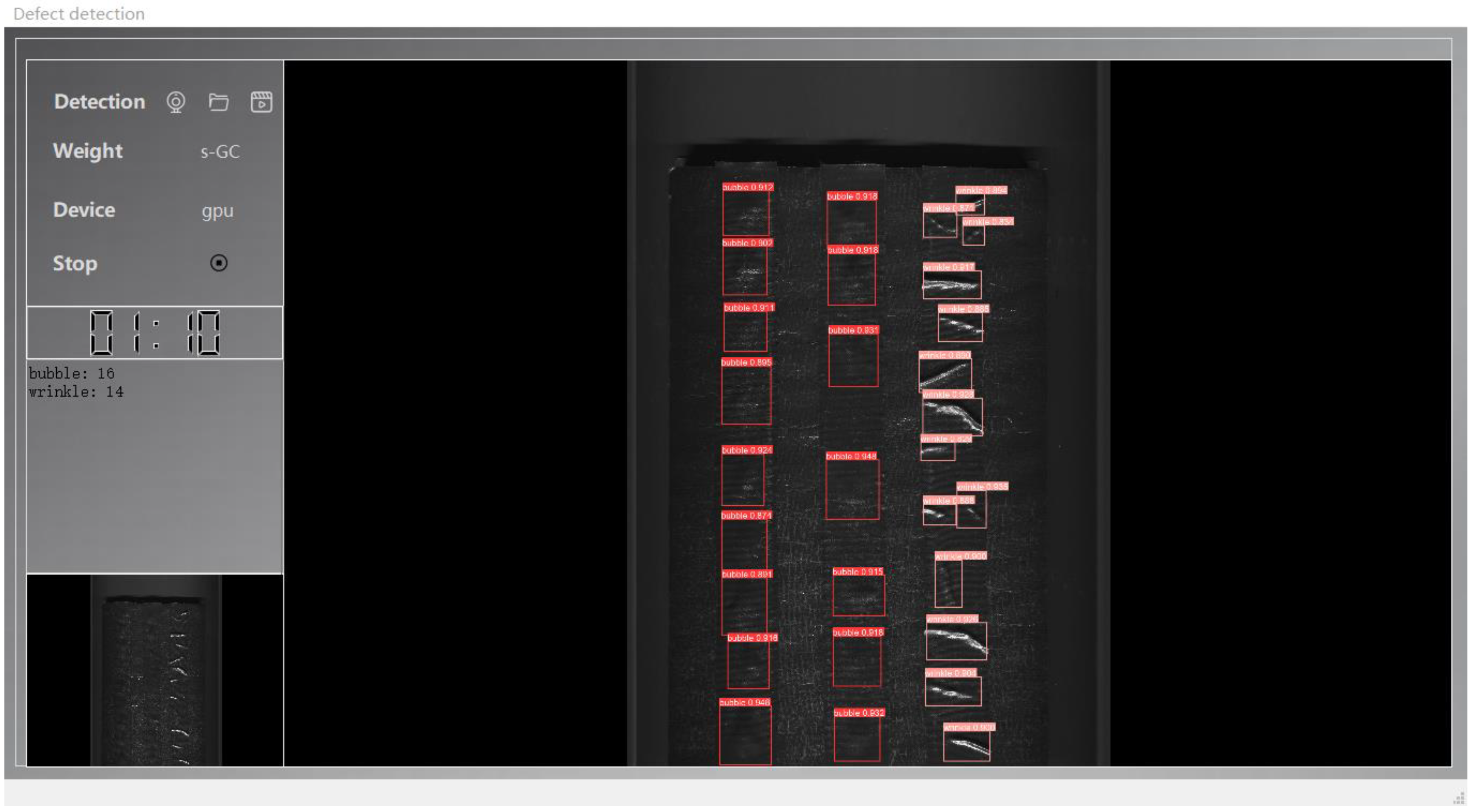
At present, there are no relevant reports in the literature on the detection of surface defects in preforms, and there is a lack of corresponding research. In order to solve the problem of high reflective characteristics of the surface of preforms based on fiber prepreg, as well as the need for online and high-precision recognition of various defects during the preform process, we proposes a method for identifying defects on the preformed surface based on machine vision and improved YOLOv5 network model. Based on the established machine vision platform, the surface image of the preform during the preforming process is obtained. In actual surface defect detection of preforms, samples exhibit the characteristics of extremely small samples and imbalanced samples. Then, the idea of transfer learning is used, and the Ghost Bottleneck module is introduced to lightweight design the YOLOv5 model. In order to improve the defect recognition accuracy, the coordinate attention module is introduced to achieve a good balance between recognition accuracy and recognition speed. Compared to before the improvement, the improved model has faster recognition speed and higher recognition accuracy.

2. Analysis of Surface Defect in Preforms and Machine Vision Platform

The surface of the preform after preforming may produce defects such as overall dislocation, wrinkles, bubbles, and dislocation of stiffener, as shown in Figure 1. Among the above defects, the common shape, common location, size, and characteristics of each type of defect are different. In order to accurately and quickly identify different defects, it is necessary to analyze common defects, understand preliminary features, and determine the required hardware parameters of the machine vision platform based on the characteristics of the defects.

Table 1. Common defects and characteristics of preform surface.

Defect Type	Common States	Common Locations	Main Cause
Dislocation of prepreg	Edge interlacing between prepregs	Edge of preform	Inconsistent orientation of multi-layer prepreg
Dislocation of stiffener	Stiffener staggered with the edges of the preform	Stiffener edge	Reinforcement direction paving error
Wrinkle	Strip protrusion	Anywhere	Uneven drag force
Bubble	Irregular circular protrusion	Except for edge position	Residual air in interlayer

shows the analysis of common defects. Among them, background texture features will be helpful for the extraction and recognition of defect features. Fully obtaining the texture features of the preform, a higher pixel image will help improve the accuracy of recognition. In order to facilitate the simulation of defects in the preforming process, the JY201 glass fiber plain woven prepreg from Tai’an Joy Company with good formability at 0–40 degrees was used. The width of its fiber bundle is about 2.3 mm, and the spacing between two warp or weft bundle is 0.2 mm. In order to better capture features, the camera’s resolution index is increased by one level, with a minimum resolution requirement of 0.1 mm.

To complete the acquisition of images, it is necessary to equip a camera and lens that meet the requirements of accuracy, width, and other requirements; and combine appropriate light sources to ensure that the object being photographed has a relatively ideal brightness. In addition, consider the triggering method of image acquisition to obtain high-quality images. The linescan camera, lens, light source, and encoder are selected; and the models are MV-CL084-91GM, MVL-LF2528M-F, MV-LTHS-800-W, and E6B2-CWZ6C-2000P/R. The parameters of the camera and lens are shown in

Table 2. Parameters of linescan camera.

Resolution	Line Frequency	Pixel Size	Communication Interface	Exposure Time	Trigger Method
8K	Convention: 14 kHz@Mono 8	5 µm	GigE	3 μs~10 ms	Internal or external

and

Table 3. Parameters of lens.

Focal Distance	F-Number	RIS Mode	Interface Type	Image Size	Optical Distortion	Working Distance Range
25 mm	F2.8–F16	Hand movement	F-Mount	Φ43.2 mm	0.40%	125~728 mm

. The visual platform built in this article is shown in Figure 2.

3. YOLOv5 Network and Improvement

In this article, the surface image of preform is obtained by the machine visual platform, and the image is annotated by the online annotation tool Make Sense. After the annotation is completed, it is saved as a txt file in YOLO format, and a dataset is created. Based on the idea of transfer learning, the YOLOv5 model is introduced to properly train the dataset and identify defects. A total of 427 images with defects were collected, and the original image resolution was 8192 × 13,000 pixels. Each image may contain multiple defects, with a total of 2157 marks. Among them, 162 overall dislocation of prepreg, 168 overall non dislocation of prepreg, 158 dislocation of stiffeners, 162 normal stiffeners, 855 wrinkles, and 652 bubbles are marked. That is, the proportion of wrinkle defects is about 40%, the proportion of bubble defects is about 30%, the proportion of reinforcement dislocation defects is about 7.5%, and the overall dislocation defects of prepreg are about 7.5%. There are differences in the number of different defect types. Compared to other open data sets, the data set established in this article has very few samples, and there are various cases of uneven samples between classes, which poses a great challenge to defect identification.

3.1. Network Structure of YOLOv5

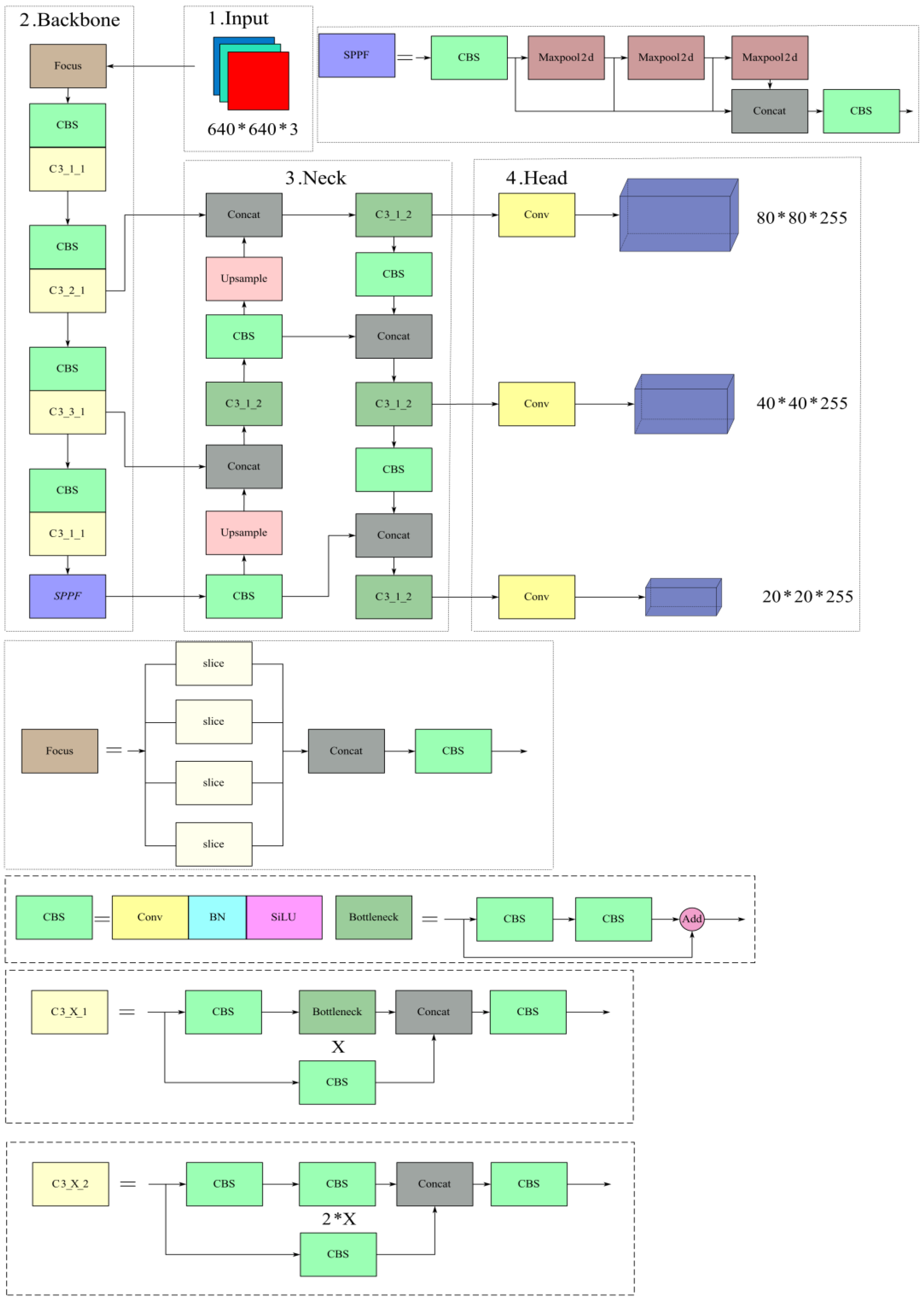
YOLO series algorithms have a fast detection speed, a high average detection accuracy, and a strong migration ability, which can be applied to other new fields. YOLOv5 is a development based on YOLOv4 and is currently widely used in the field of target detection [16,17,21]. YOLOv5 is an object detection architecture and model that has been pre trained on COCO datasets, including several different series. In the official code, there are four versions that are more mature and widely used, namely the YOLOv5s, YOLOv5m, YOLOv5l, and YOLO5x models. YOLOv5 uses the C3 module and SPPF module as the backbone, FPN + PANet as the neck, and YOLOv3 head as the detection head. In addition, it also uses various data enhancement methods and some modules from YOLOv4 for performance optimization. The network structure of YOLOv5s is shown in Figure 3.

3.2. Improved Methods

In practical industrial applications, the surface images of preforms have the characteristics of high noise and high background similarity, which brings difficulties to the recognition of defects. In order to make the model focus on the feature information of the surface defects of the preform, we introduce coordinate attention module into the YOLOv5 model. After introducing the attention mechanism, it will increase the parameters and models, and may increase the reasoning time. In order to meet the requirements of real-time detection and embedded system deployment, we consider using lightweight methods to process the network structure based on the use of CA modules and introduce the Ghost Bottleneck module.

3.2.1. Coordinate Attention Module

Attention mechanisms are more effective for general classification tasks and are widely used in various neural networks. Currently, channel attention mechanisms such as the SE module and hybrid attention mechanisms such as the CBAM module have been applied [38,39]. However, SE only encodes information between channels, ignoring equally important spatial relationships. The CBAM module obtains location information by reducing the channel dimension of the input tensor, and then uses convolution to calculate spatial information. However, it can only extract the rejection relationship of the feature map and cannot extract the long-distance dependency relationship.

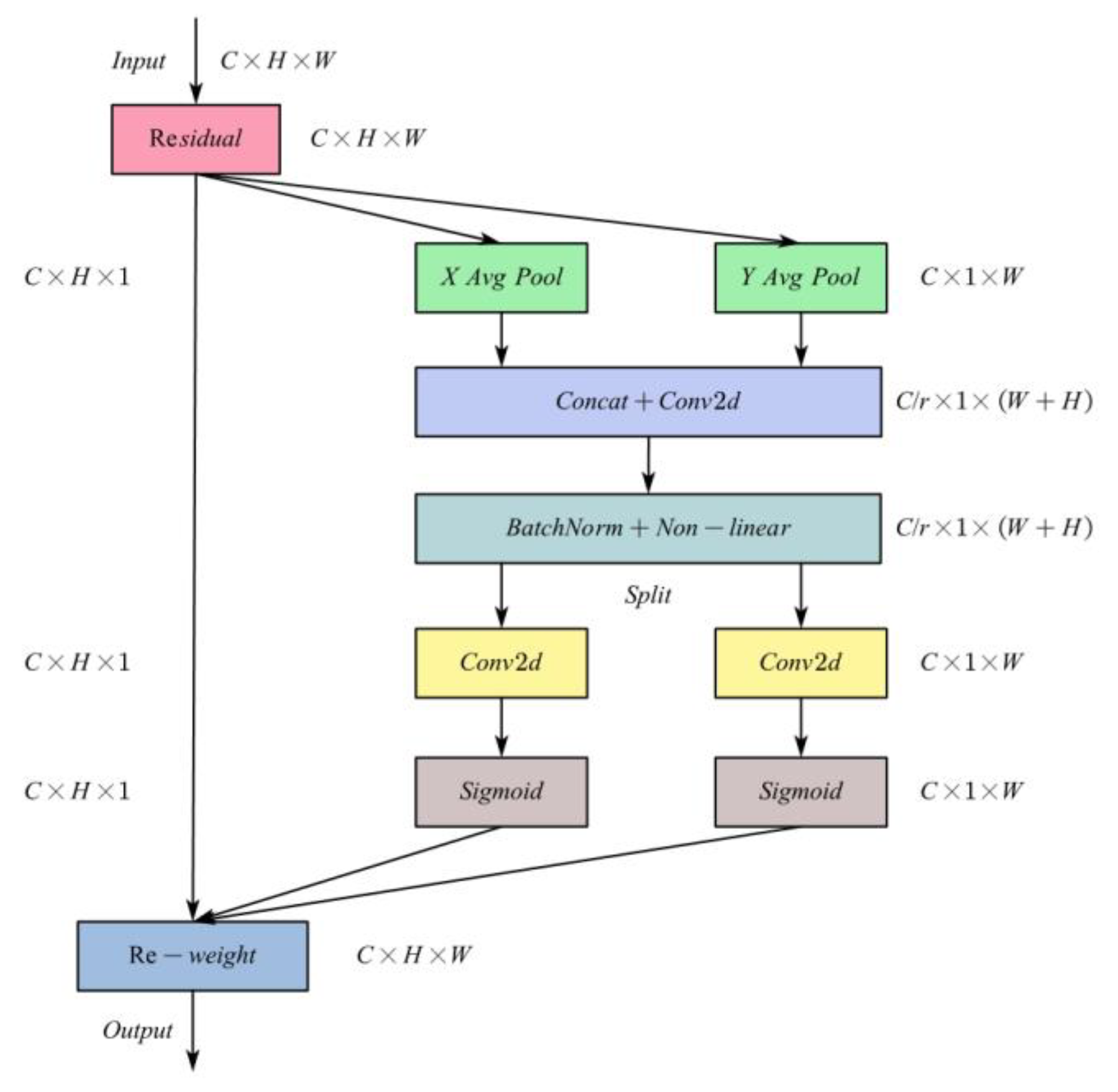
The attention module can convert any intermediate feature tensor $X=\left[x_1,x_2,x_{\mathrm{c}}\right]\in R^{\mathrm{C}\times \mathrm{H}\times \mathrm{W}}$ is used as the input, and outputs a transformation tensor $Y=\left[y_1,y_2,y_{\mathrm{c}}\right]$ with the same size as $X$. $\mathrm{C}$ is the number of channels, and $\mathrm{H}$ and $\mathrm{W}$ are the height and width of the input image, respectively. The CA module structure is shown in Figure 4. The calculation process includes two parts: coordinate information embedding and coordinate attention generation [40].

In order to solve the disadvantage of encoding global pooling as spatial information for each channel in other attention modules, the CA module uses coordinate information embedding to convert global pooling into a pair of one-dimensional feature codes. Specifically, for the input $X$, we use two spatial range pool cores $(\mathrm{H},1)$ or $(1, \mathrm{W})$ to encode each channel along the horizontal and vertical coordinate, respectively. Therefore, the output of the c-th channel at height $h$ and the output of the c-th channel at width $w$ can be determined using the following expression:

$$z_c^h\left(h\right)=\frac{1}{\mathrm{W}}\sum _{0\le \mathrm{i}<\mathrm{W}} x_c\left(h,i\right)$$

(1)

$$z_c^w(w)=\frac{1}{\mathrm{H}}\sum _{0\le \mathrm{j}<\mathrm{H}} x_c\left(j,w\right)$$

(2)

By computing the two formulas, the process of aggregating characteristics takes place across two spatial directions. The result is a set of bi-directional sensing feature maps capable of capturing long-distance relationships along a single spatial direction, while maintaining precise location information along the other. This approach enables the network to more accurately locate objects of interest.

The second part is coordinate attention generation. First, connect the formulas together, and then send them to the 1 × 1 convolution function $F_1$, resulting in the following formula:

$$f=\delta \left(F_1\left(\left[z^h,z^w\right]\right)\right)$$

(3)

where $\delta$ is a nonlinear activation function, $f\in R^{\mathrm{C}/r\times (\mathrm{H}+\mathrm{W})}$ is an intermediate feature map encoding spatial information in the horizontal and vertical directions, and $r$ is the ratio of down sampling. Then, we split $f$ into two independent tensors along the spatial dimension, $f^{ h}\in R^{\mathrm{C}/r\times \mathrm{H}}$ and $f^{ w}\in R^{\mathrm{C}/r\times \mathrm{W}}$. The other two 1 × 1 convolutional transformation functions $F_h$ and $F_w$ are used to transform $f^{ h}$ and $f^{ w}$ into tensors with the same channel number for input X, respectively:

$$\begin{array}{c}{g}^h=\sigma \left(F_h\left(f^{ h}\right)\right)\\ g^w=\sigma \left(F_w\left(f^{ w}\right)\right)\end{array}$$

(4)

where $\sigma$ is sigmoid function. The outputs $g^h$ and $g^w$ are expanded and used as attention weights, respectively. Finally, the output of the CA module can be written as:

$$y_c\left(i,j\right)=x_c\left(i,j\right)\times g_c^h\left(i\right)\times g_c^w\left(j\right)$$

(5)

3.2.2. Ghost Bottleneck Module

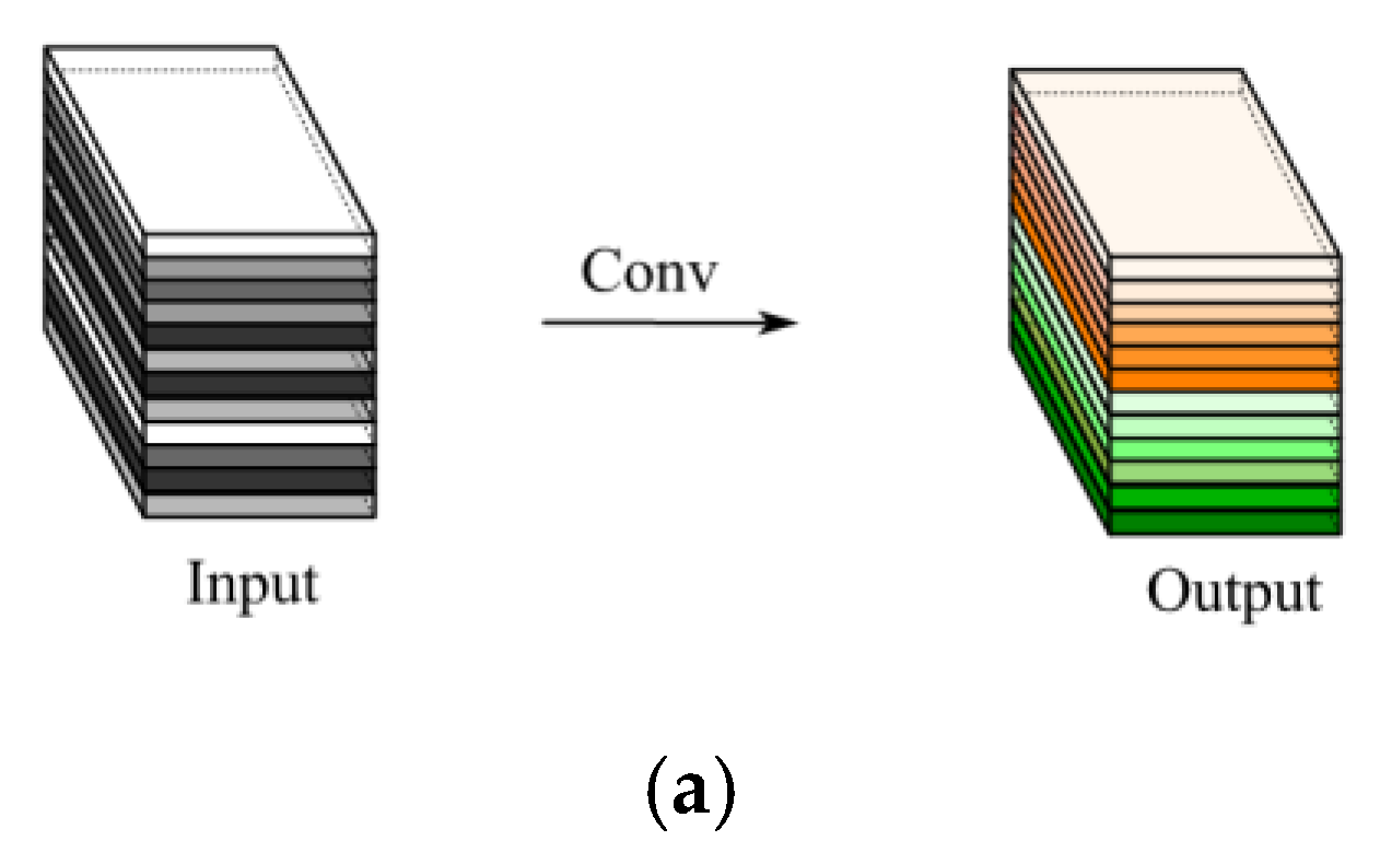
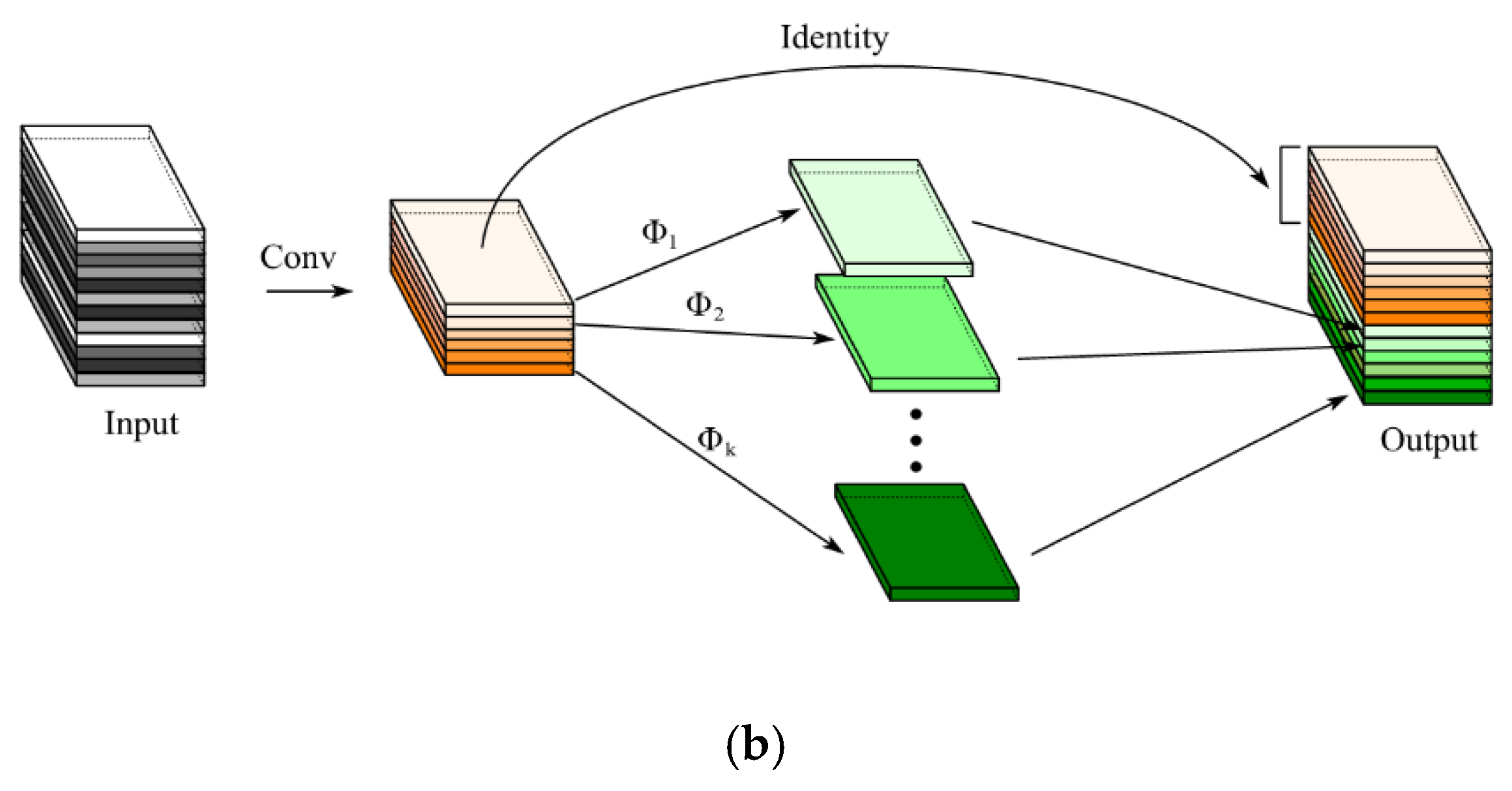
The Ghost lightweight module is the main part of the Ghost net network model proposed by Huawei Noah’s Ark Laboratory in 2020 [41]. It applies the channel attention mechanism and has been widely used [35,38]. From Figure 5, (a) is a normal convolution module and (b) is a Ghost module. The calculation step of the Ghost module is that the necessary features of the input features are obtained by 1 × 1 convolution; then, a similar feature map (Ghost) of the features is obtained by depth separable convolution; and finally, the two channels are spliced. There are super parameters s and d in the Ghost module, and the different settings have an impact on the accuracy and volume scale of the improved network. Based on the comparative experimental results in literature [41], we select the settings of s = 2 and d = 3.

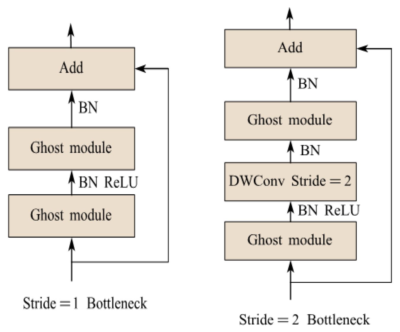
The Ghost module retains residual blocks, and there are two types of Ghost Bottleneck network structures. As shown in Figure 6, the Ghost Bottleneck is composed of two Ghost modules stacked together. The first Ghost module is used for channel expansion and increasing the number of channels, while the second Ghost module is used to reduce the number of channels. The ReLU activation function is not used after the first Ghost, but BN and ReLU are applied to other layers. If stride = 1, the feature map size remains unchanged. If the stride = 2, a depth convolution with a step size of 2 between the down sampling layer and the two Ghost modules is used to reduce latitude and achieve a direct shortcut path.

Since the deep convolution operation with stride = 2 adds feature information, its detection speed is slow. Therefore, this article selects the Ghost Bottleneck structure with a stride = 1 for lightweight design, which can improve the detection speed.

3.2.3. Improved Network Structure of YOLOv5-GC

We will carry out lightweight design in the network structure of YOLOv5s while considering the improvement of detection accuracy. For lightweight design, considering factors such as model size and detection speed, a Ghost Bottleneck module with stride = 1 is used to replace the Bottleneck module of C3_X_1 in the backbone network, constituting a C3Ghost_X module, still comprising CSP architecture; using the Ghost Bottleneck module instead of C3_X_2 modules in the neck to reduce the complexity of the model and achieve a lightweight network. Due to the fact that the feature extraction of the YOLOv5s network is mainly completed in the backbone network and the attention mechanism module can enhance the ability of the network model to obtain initial features, this article adds the CA module to the backbone network and places it after the C3Ghost_X module; the addition of the CA module can extract more features on the connection channel and improve the detection accuracy of the improved model. The improved network model is named YOLOv5s-GC, and its network structure is shown in Figure 7.

3.2.4. Evaluation Indicators

There are many indicators commonly used to measure algorithm performance in target detection. In order to facilitate comparison, this article uses indicators such as accuracy precision, recall, mean average precision (mAP), and inference time to measure prediction performance.

Precision is an indicator used to evaluate the performance of a classification model, which refers to the ability of a classifier to accurately identify positive examples during prediction. The formula is as follows:

$$\mathrm{Precision}=\frac{\mathrm{TP}}{\mathrm{TP}+\mathrm{FP}}$$

(6)

where TP represents true positive, i.e., the number of samples that are positive and are predicted to be positive; FP represents a false positive example, which is the number of samples that are negative examples that are incorrectly predicted as positive examples.

Recall is used to evaluate the ability of the model to find all positive samples, reflecting the ratio of all actual positive samples found by the model. Its calculation formula is:

$$\mathrm{Recall}=\frac{\mathrm{TP}}{\mathrm{TP}+\mathrm{FN}}$$

(7)

where FN represents a false negative, which is the number of samples that are positive and incorrectly predicted to be negative.

AP is an important performance indicator in classification tasks. When measuring model performance, precision and recall are two mutually constraining performance indicators. These two indicators have the limitations of single point values and cannot fully evaluate the overall performance of the model. Therefore, the introduction of AP enables a full trade-off between precision and recall to comprehensively evaluate the performance of the model. Using precision as the ordinate and recall as the abscissa, we can obtain a P–R curve. The area between the P–R curve and the coordinate axis is the value of AP. The expression is:

$$\mathrm{AP}=\frac{1}{n}\sum _{k=1}^n P(k)·\mathit{rel}(k)$$

(8)

where $P\left(k\right)$ represents the accuracy of the first k prediction results, while $\mathit{rel}\left(k\right)$ is a function that represents the correlation of the k-th prediction results, where k ranges from 1 to n; and n is the total number of prediction results.

mAP is used to measure the accuracy of the system. In a multi-classification task, each category can calculate its own AP value, and averaging these values can obtain the mAP value of the entire dataset. Typically, mAP values calculated at a threshold of 0.5 are often used to evaluate the performance of a model, also known as mAP@0.5. mAP@0.5:0.95 refers to calculating the mAP values under each threshold by changing the threshold value from 0.5 to 0.95 in steps of 0.05 and averaging all the mAP values to comprehensively evaluate the performance of the model under different IoU thresholds. The calculation formula is:

$$\mathrm{mAP}=\frac{1}{N_c}\sum _{i=1}^{N_c} \mathrm{A}{\mathrm{P}}_i$$

(9)

where $N_c$ indicates the number of categories, and $\mathrm{A}{\mathrm{P}}_i$ represents the average precision of the ith category. Add up the AP values for all categories and divide by the number of categories; $N_c$ gives the value of mAP.

In order to evaluate the performance of the model more comprehensively, inference time is introduced, which refers to the time required to recognize the target and output the results after inputting the image into the algorithm. Inference time is one of the important indicators to measure the practicality and real-time performance of defect recognition based on the YOLO model.

4. Results and Discussion

4.1. Experimental Environment

In this article, we first annotate the images to create a dataset, process the image size in the dataset, and batch compress the images to a size of 640 × 640 pixels; then, set training parameters to ensure better training effects and consistent training conditions; and then, send them to different network models for training and analysis of the results. Finally, we save the model for testing and deployment. The surface defect detection of preforms based on Yolov5 in this article uses the PyTorch framework, and the graphics card model used is NVIDIA Geforce RTX 3080. The detailed configuration is shown in

Table 4. System hardware and software configuration.

Environment	Configuration Name (Version)
Operating system	Ubuntu (16.04.7)
Deep-learning Framework	PyTorch (1.11)
CPU	Intel(R)Core(TM)i9-9900K CPU (3.60 GHz)
Memory	32 GB
GPU	NVIDIA GeForce RTX 3080 (10G) × 2
Compiler	Python (3.9.0)
Acceleration module	CUDA (11.1.1)

.

In order to obtain better detection results, it is necessary to determine the hyperparameters in the training file and make subsequent adjustments accordingly. Some studies have shown that hyperparameters such as initial learning rate and weight decay may affect the detection performance of training models. However, as YOLOv5 is already a mature target detection model and has achieved excellent prediction performance in the field of natural images, the setting of hyperparameters is not the focus of this article. In this article, we set the parameters based on the training of large-scale datasets, as shown in

Table 5. Setting of some hyperparameters.

Parameters	Value
lr0	0.001
lrf	0.1
Momentum	0.937
Weight_decay	0.0005
Epochs	200
Optimizer	Adam
Image_size	640 × 640 × 3

.

4.2. Prediction Performance of YOLOv5

The reason for the small number of samples in the self-collected dataset in this article is that in actual production, there are very few samples that can be collected with surface defects. In order to meet this practical situation, there are fewer samples in the self-collected dataset. This article investigates the impact of sample size on model convergence and recognition accuracy in the sample set; choose approximately 50%, 75%, and 85% of 427, respectively. Corresponding to the proportion of the number of images, the number of marked defects is also basically consistent. A sample set with 203, 306, 352, and 427 images was selected for experimental research, and the proportion of various defects remained consistent with the proportion in Section 3. The smaller YOLOv5s model is selected for training and testing, and the loss function obtained is compared with the prediction accuracy, as shown in Figure 8 and

Table 6. Comparison of prediction performance under different sample numbers.

Number of Samples	P	R	mAP@0.5	mAP@0.5:0.95
203	0.715	0.834	0.801	0.536
306	0.735	0.864	0.817	0.593
352	0.882	0.896	0.951	0.693
427	0.915	0.912	0.952	0.704

. It can be found that the prediction performance of 352 image datasets and 427 image data is generally better than that of less samples. The predictive performance of the model on the 427 image dataset is slightly better than that on the 352 sample dataset, but the difference is not significant. So, when the sample size is 427, it can be considered a suitable small sample dataset. According to this trend, if the number of sample sets is further increased significantly, the recognition effect will generally be better. However, this article focuses on the problem of defect recognition under extremely small samples, so the sample size is not suitable for further expansion.

On this basis, we train the four models of the YOLOv5 series and analyze their performance. After training each model, the total loss function curve of each model is shown in Figure 9. The total loss function values of each model in the training set decreased to below 0.05 after 200 training rounds, all remaining in a relatively low state, and there was no overfitting. Therefore, it is reasonable to use YOLOv5 series models to detect surface defects on preforms.

The prediction performance of the four models was evaluated on the test set, and the results obtained are shown in

Table 7. Comparison of model size and prediction performance of YOLOv5.

Model	P	R	mAP@0.5	mAP@0.5:0.95	Inference Time/ms	Weight Size/MB
5x	0.924	0.904	0.955	0.702	17.3	165
5l	0.932	0.925	0.962	0.711	14.9	88.5
5m	0.938	0.907	0.959	0.697	12.1	40.2
5s	0.915	0.912	0.952	0.704	9.7	13.7

. Among them, for the larger YOLOv5l model, the prediction indicators in this training set are the best, but the model has a larger scale and a longer inference time. The YOLOv5s model has the smallest scale, the shortest reasoning time, and various indicators are in the middle. In order to balance the prediction performance, reasoning time, and portability of the model, the YOLOv5s model is a better choice. We will take the YOLOv5s model as the research object, and based on this model, carry out network improvement and optimization, lightweight design, and improve recognition accuracy.

4.3. Performance Comparison before and after Model Improvement

According to the method of model improvement, they are named 5s, 5s-G, 5s-GC, and 5s-C, and the improved model is trained and tested; compare the performance on the training set, as shown in Figure 10. The size and predicted performance of each model on the test set are shown in

Table 8. Comparison of model size and prediction performance before and after improvement.

Model	P	R	mAP@0.5	mAP@0.5:0.95	Inference Time/ms	Weight Size/MB
5s-C	0.958	0.959	0.976	0.732	11.5	13.9
5s-GC	0.947	0.926	0.956	0.726	7.2	7.7
5s-G	0.882	0.896	0.948	0.691	6.7	7.5
5s	0.915	0.912	0.952	0.704	10.3	13.7

.

Through comparison, it was found that the addition of the attention mechanism CA helped improve the detection accuracy of defects. When added alone, the accuracy rate increased by 0.043, the recall rate increased by 0.047, mAP@0.5 increased by 0.024, mAP@0.5:0.95 increased by 0.028, but the reasoning time and model weight increased; the addition of the Ghost Bottleneck module reduced the system size and reasoning time, but the accuracy index decreased. The combination of the two reduces the weight of the improved network model by 43.8%, the inference time by 30.1%, and the average accuracy compared to the previous improvement; mAP@0.5:0.95 improved by 0.022, comprehensively improving the model size, inference time, detection accuracy, and other aspects. We compared the detection results of 5s and 5s-GC models on some test sets, as shown in Figure 11. On the model of YOLOv5s before improvement, there are errors and omissions in the recognition of test sets after training. On the improved YOLOv5s-GC model, these situations were improved, and the confidence level of recognition improved; in addition, the overall recognition effect improved.

Based on the YOLOv5 series model, the detection performance on benchmark datasets or large-scale self-collected datasets has been applied and explained in many pieces of literature [33,34,35]. However, there is currently no research on the detection performance for extremely small and imbalanced samples. This article focuses on defect detection in the case of extremely small and imbalanced samples. The testing of YOLOv5 in defect detection on self-collected datasets in this chapter also demonstrates that YOLOv5 performs well on self-collected datasets, indicating that the detection performance of YOLOv5-based models on self-collected datasets is similar to that of other benchmark datasets or self-collected datasets. Therefore, the effectiveness verification of YOLOv5-based improvement methods based on self-collected datasets can be trusted.

4.4. Deployment of Models

The trained model has been deployed to the MXE-5501 industrial computer (with a CPU of i7-6820EQ, 8 GB of memory, and a solid-state drive capacity of 480 G), with the following steps:

(1)

Install the CPU version of PyTorch. According to the processor architecture of MXE-5501, install the corresponding PyTorch version. Due to the x86 CPU of this device, it is necessary to install the CPU version of PyTorch;

(2)

Install Python and OpenCV. Install Python 3.9 and OpenCV 4.1.1 on MXE-5501;

(3)

Clone Yolov5 code. Clone the required code onto MXE-5501;

(4)

Modify the yolo.py and common.py files and add interface files for detection. Modify the yolo.py and common.py files to adapt to the environment on MXE-5501, and develop interface files for detection using PyQt5, as shown in the Figure 12.

After deployment on industrial control computers, online detection of surface defects on preforms can be achieved.

The detection model deployed on an industrial computer consists of three steps in the workflow: camera image detection, folder image detection, and video detection. The linear array camera captures a complete image every second and saves it in a fixed folder. Open the Yolov5 detection interface, select the function of the detection folder, select the device as CPU, and select the corresponding model. The program will determine if there are any new files in the folder. If there are any new files, the detection will continue. If there are no new files, the previous detection results will remain.

We used a visual platform as a simulation platform to obtain images and serve as a preliminary validation for online testing. According to current testing data, the time for online shooting and defect identification before improvement was 2236 mm; after improvement, the online shooting and defect recognition time was 1965 ms, and the recognition time was reduced by 331 ms, resulting in a significant improvement in detection speed.

5. Conclusions

In this paper, a machine vision platform is built to collect surface images of preforms, and a sample set for defect labeling is established. A rapid and accurate method for obtaining surface defect recognition of preforms is proposed. Aiming at the issue of real-time detection of surface defects in prepreg materials with extremely small and imbalanced samples, this paper proposes the use of a coordinate attention mechanism to obtain spatial and distance dependencies, thereby improving the ability to obtain defect features. The lightweight Ghost Bottleneck module is used to reduce the scale of the model and achieve accurate and rapid detection of various defects on the surface of the preform. One of the main differences between YOLOv5 and improved YOLOv5 is the use of Ghost Bottleneck modules instead of traditional convolution, reducing model size and improving detection speed. Another difference is that in YOLOv5’s backbone network, a coordinate attention mechanism is adopted to improve the ability to obtain features. In this paper, 2157 defects in 427 images were marked and model training was conducted. The effectiveness of the improved model was verified by comparing the scale, detection accuracy, inference time, and other indicators of the model before and after improvement.