Sports Risk Prediction Model Based on Automatic Encoder and Convolutional Neural Network

Abstract

In view of the limitations of traditional statistical methods in dealing with multifactor and nonlinear data and the inadequacy of classical machine learning algorithms in dealing with and predicting data with high dimensions and large sample sizes, this paper proposes an operational risk prediction model based on an automatic encoder and convolutional neural networks. First, we use an automatic encoder to extract features of motion risk factors and obtain feature components that can highly represent risk. Secondly, based on the causal relationship between sports risk and risk characteristics, a convolutional neural network with a dual convolution layer and dual pooling layer topology is constructed. Finally, the sports risk prediction model is established by combining the auto-coded feature components with the topology of the convolutional neural network. Compared with other algorithms, the proposed method can effectively analyze and extract risk characteristics and has a high prediction accuracy. At the same time, it promotes the integration of sports science and computer science and provides a basis for the application of machine learning in the field of sports risk prediction.

1. Introduction

Nowadays, under the advocacy of the state and government, sports have gradually become universal, normalized, and an indispensable part of people’s lives. However, due to a lack of basic knowledge of sports mechanisms, methods, approaches, processes, and intensities, sports-related risk events such as injuries, diseases, and even sudden death often occur, which seriously affect people’s physical and mental health and even threaten their lives. In view of this, in the face of many potential sports risk factors, correctly analyzing and predicting sports risks and building a personalized sports risk warning mechanism is not only an important task for current sports researchers but also has practical significance for the construction of “personalized” physical fitness guidance methods with population characteristics and strong targeting. It is of practical significance.

In previous studies, many scholars studied and analyzed the causes of sports risk from different disciplinary perspectives. Although they can better simulate and explain the risk mechanism in theory, there is a large heterogeneity between different studies, which makes it difficult to determine effective prevention strategies. Quatman [1], a scholar, believes that this contradiction is related to specific research paradigms and suggests that multidisciplinary research models be used to study sports risk. With the vigorous development of computer application technology and the application of big data in the field of natural science research, natural science research is undergoing a transformation from empirical science, theoretical science, and computing science to data science. Machine learning has been widely used in various fields and has made great progress because of its powerful data processing and data mining abilities. Therefore, using machine learning methods to study sports risk has great potential. It can not only provide prediction information for sports risk prevention but also promote the development of digital sports training, digital fitness guidance, and sports risk early warning. At present, the application of machine learning in sports risk research mostly focuses on competitive athletes. The algorithms involved in the research are mainly random forests, neural networks, support vector machines, decision trees, etc.

The occurrence of sports risks is the result of multiple factors. Meeuwisse et al. [2] summarized sports risk factors into three parts: internal risk factors, external risk factors, and induced events. Meeuwisse pointed out that the best way to prevent sports risks is to eliminate all risk factors that may lead to risks from the inside out as much as possible before sports. However, when traditional statistical methods are used to establish multiple linear regression models, in order to ensure the stability and repeatability of the model, the number of predictors must be less than the sample size, and the predictors must be gradually independent of each other. These problems lead to the multiple regression of traditional statistics, which cannot make good use of potential predictors and cannot fully mine the data. As a new statistical method, machine learning can capture the interaction effect between various predictors, providing a basis for the identification of sports risk factors and the research of risk etiology. Talukder et al. [3] used the random forest algorithm to model and predict the tactical statistics and risk situation of NBA players in two seasons and extracted five important sports risk prediction characteristics through the random forest algorithm: the average speed of athletes in the game, the number of games played by athletes in the season, the average running distance in the game, the average playing time in each game, and the average score in each game. Bryan et al. [4] studied the data and risk of 2322 hockey players from 2007 to 2017. They used the variance expansion factor to conduct multiple collinearity evaluations on each prediction factor and selected XGBoost to model it. By using SHAP (Shapley Additive Explanations, SHAP) scores to evaluate and explain the prediction factors, Bryan et al. extracted a total of 38 players’ risk prediction factors and 15 goalkeepers’ risk prediction factors, which can predict sports risk well. Jauhiainen et al. [5] used random forest to model the demographic parameters, sports ability parameters, physical examination parameters, and non-contact risk of basketball players and floor tennis players based on logical regression and tried to use the predictive ability of machine learning to detect sports risk factors. The research results show that although the accuracy of random forest and logical regression in predicting sports risk is not satisfactory, the sports risk factors detected by random forest and logical regression algorithms are consistent with those reported in previous explanatory studies. Jauhiainen et al. pointed out that although the prediction accuracy of the model established in the study is still relatively low, machine learning methods can be used to detect sports risk factors and prove the prediction ability of risk factors found in previous explanatory studies. Applying machine learning to analyze sports risk factors can help us understand the mechanism of sports risk, better detect the risk prediction factors with predictive ability, and lay the foundation for sports risk prevention research.

The occurrence of sports risk is often due to the internal risk of patients themselves, which makes them susceptible to risk and exposed to external risk, and the risk results are formed under the effect of induced events. If the patient’s sports risk and risk propensity can be predicted in advance, timely adjustments can be made to avoid the occurrence or further aggravation of sports risk. Rossi et al. [6] used GPS-based external monitoring means of training load to track and monitor football players for 23 weeks and established a non-contact risk prediction model using three different algorithms: decision tree, random forest, and logical regression. By comparing the performance of decision tree, random forest, and logistic regression in sports risk prediction, it is found that decision tree classifiers can detect about 80% of the risk with about 50% precision, which is far better than random forest. Although the prediction accuracy is not satisfactory, the prediction model still reduces the risk-related expenses for Barcelona Football Club. Gao Xiaolin et al. [7] established the non-contact risk multilayer perceptron (MLP) neural network model of Chinese football players using age, sex, and other demographic data and action pattern screening evaluation score data and believed that the application of the MLP neural network in sports risk prediction has a good prospect. The author believes that although the overall prediction accuracy of the model is good, the prediction accuracy of the disease-free situation is poor, which may lead to the high specificity of the model, which is not easy to deploy in practice. At the same time, there are problems such as a small sample size, which makes the network difficult to converge. Bryan et al. used the XGBoost algorithm to model the risk prediction of 2322 hockey players. The model showed high prediction accuracy in the sports risk prediction of hockey players at different positions, which made Bryan think that regression analysis should not be the only standard for risk prediction analysis. Rommers [8] and others conducted a pre-season test on 734 football players aged U10 to U15 based on anthropometry and sports ability tests and established a risk prediction model with a precision rate of 84% using XGBoost according to the pre-season test results. When the model is tested on 147 athletes’ test data, recall, precision, and F1-scores are all 85%, which means that the precision and sensitivity of the model are reasonable. Rommers pointed out that machine learning has a good prospect for the risk assessment of excellent athletes. Machine learning can be applied to the formulation of risk prevention strategies to identify athletes with high risks.

To sum up, the research on the application of machine learning to sports risk mainly focuses on the identification of sports risk factors and the prediction of sports risk. The application of machine learning in sports risk prevention research not only makes up for the limitations of traditional statistics in dealing with multifactorial and nonlinear data but also can more completely show the original appearance before sports risk, providing a basis for clinical risk assessment and coaches to adjust training timely [9]. At present, the application of machine learning in sports risk prediction has attracted great attention in the field of sports science [10]. According to the existing research reports, the problems in the current research are as follows:

(1)

The sample size is small. The application of machine learning to the study of sports risk requires a sufficient sample size. If the sample size is small, it is easy to have problems such as difficulty obtaining data features and poor generalization ability of the model [11]. However, the research in this field has just begun, and there are still few domestic studies in this field. There are factors such as insufficient investment in project funds and manpower, a lack of a unified risk information management system in sports team management, and a poor connection between athletes’ training and the working modes of coaches and team doctors that lead to difficulties in data collection and the failure to obtain a sufficient sample size.

(2)

The integration of disciplines is insufficient. At present, the research in this field in China is relatively weak. Because the discipline connection is not close enough, scientific researchers with computer discipline backgrounds know very little about professional knowledge in the field of sports science, and scholars with sports discipline backgrounds cannot complete complex programming, which leads to problems such as the lack of interpretation of risk factors [12], making the development of machine learning in this field slow. Promoting the development of multidisciplinary cooperation will further promote the development of sports science and sports medicine.

(3)

The practical application rate is low. Using machine learning to analyze and mine the data generated in the training process of athletes can reveal the development trend of athletes’ physical functions, assist coaches and team doctors in making decisions based on data, timely adjust the intensity and capacity of training, and avoid risks [13]. However, due to the late development of research in this field and the lack of research reports, it is not possible to better combine other application technologies to generate applications and apply them to practice.

In view of the above shortcomings, this paper proposes a sports risk prediction model based on an automatic encoder and convolutional neural network to process and predict high-dimensional, large-sample sports risk data, aiming to promote the integration of sports and computer science and provide a basis for the application of machine learning in the field of sports risk prediction.

2. Overview of Relevant Theories

This chapter will introduce the relevant theories of the methods used in this study.

2.1. Concept of Sports Risk

Currently, for research purposes, many scholars have developed a description and definition of the concept of exercise risk, mainly in terms of the analysis of exercise risk event factors and consequential effects. In the analysis of risk factors for sports events, the causes of risk are categorized as sports load, sports environment, and personal factors. First, improper handling and injury risks during exercise may lead to physical injuries, and minor injuries may affect daily life and work, while serious injuries may lead to disability and even life-threatening injuries. Secondly, sports-risk events can have a negative impact on the psychology of the exerciser, such as fear, anxiety, and depression. At the same time, some sports-risk events can lead to financial losses, such as medical expenses, expenses for post-rehabilitation, and the inability to work or reduced income due to injury or disability. Finally, serious sports risk events may have a negative impact on society, such as triggering public dissatisfaction or a boycott of the sport and affecting the development of related events or programs.

Exercise is a form of fitness with the goal of promoting physical health. Exercise risk is a side effect of healthy exercise and is present in any type of sport. A risk is the likelihood of an event occurring, that is, an event that could occur but has not yet. Exercise is unique in that it is a dynamic process of interaction between man and nature, human society, and man himself, and this process is uncontrollable; that is, in the dynamic process of exercise, exercise risk is bound to exist and is unavoidable. Due to the specificity of sports, the process is uncontrollable, so the risk must exist objectively in all aspects of the sports process. Once sports risks occur, they will inevitably have an impact on sports safety and sports purposes. Risk events in sports are triggered by different risk factors, which are expressed as risk losses. If there were no risk events, there would be no carrier for risk causation, and the corresponding risk losses would not occur.

Based on the summary and analysis of studies related to sports risk and the concept of sports risk, sports risk can be understood as a variety of potential hazards and health risks that arise when performing sports and exercise, which may adversely affect the physical health of the exerciser and even lead to serious sports injuries and accidents. Exercise risks may originate from many sources, including exercise methods, exercise environments, individual physical differences, and inappropriate behavior during exercise. In-depth understanding and reduction of exercise risk are essential to improving exercise effectiveness and safeguarding exercise health. For this reason, exercise risk assessment and management has become a popular area of research.

2.2. Introduction to Relevant Algorithms and Technologies

2.2.1. Resampling Method

The problem of unbalanced datasets is extremely common in machine learning and data mining, especially for problems such as classification and clustering [14]. An unbalanced dataset is one in which the number of samples in one or some categories far exceeds the number of samples in other categories, which can lead to models that are better at prediction for the more numerous categories but perform poorly for the less numerous categories. Therefore, it is particularly important to solve the problem of unbalanced data sets. The resampling technique is one of the most effective ways to solve the unbalanced dataset problem by increasing the sample size of the minority class and its proportion, thus making it easier for the classifier to identify the minority class. When the number of majority class samples is too large, the resampling technique can reduce its effect on the classifier by reducing the number of majority class samples, thus improving the problem of unbalanced datasets, improving the performance of the model, and making the classifier more accurate in learning the minority classes, which is very important for solving practical problems. According to the methods of balancing class distribution, resampling techniques can be divided into three categories: undersampling, oversampling, and hybrid sampling.

Undersampling methods are methods that reduce the degree of sample imbalance by reducing the number of majority-class samples or increasing the number of minority-class samples. Common undersampling methods include random undersampling, under-sampling with put-back, and prototype selection methods. In contrast to undersampling methods, oversampling methods generate new training data by performing certain transformations on the original data (e.g., rotating, flipping, scaling, adding noise, etc.). The two main types of oversampling methods are synthetic oversampling and random oversampling [15]. Hybrid sampling methods combine the advantages of both undersampling and oversampling to balance the number and proportion of data by adding samples from a few classes and removing samples from most classes while retaining as much of the original information as possible. Hybrid sampling methods usually include random hybrid sampling methods, resampling hybrid sampling methods, and data augmentation hybrid sampling methods.

2.2.2. Information Gain

Information gain (IG) is an effective feature selection method that can effectively select key features and eliminate irrelevant one. It is used to determine the contribution of each feature in the dataset to the prediction results. The measure of feature importance is to examine how much information the feature can bring to the overall sample classification. The more information, the more important the feature [16]. Then the features are sorted according to their contribution, and then the features are filtered to achieve the effect of feature latitude reduction. The experimental data are optimized to obtain the optimal index.

The definition of information entropy in information theory is as follows: if there are n possible values of variable X, which are $x_1, x_2,$…$, x_n$, the probability of each value is $p_1, p_2,$…$, p_n$, then the information entropy of variable X is:

$$H(X)=-\sum _{i=1}^n{p}_i{log}_2{p}_i$$

(1)

Formula (1) indicates that the more possible changes of X, the more information it carries. It has nothing to do with the specific value of the variable but only with the type of value and the probability of occurrence.

In the classification problem, category C is a variable, and its possible values are $C_1,C_2$, …$,$ $C_n$. The probability of occurrence of each category is $p(C_1), p(C_2),$ …$,p(C_n)$, respectively, where n is the total number of categories. At this time, the information entropy of the classification system can be expressed as:

$$H(X)=-\sum _{i=1}^{n}p(C_i){log}_{2}p(C_i)$$

(2)

Information gain is specific to a specific feature. The difference between the amount of information that the feature T system has and does not have is the amount of information that this feature brings to the system, that is, IG [17]. The information quantity of the system with feature T is calculated according to Formula (1), which represents the information entropy of the system when all features are included. If the classification system does not contain feature T, it can be calculated using Formula (2). The possible values of feature T are ($T_1$, $T_2$, …, $T_n$), so the information entropy when feature T is fixed is:

$$\begin{gathered} H(C|T)=p_{1}H(C|T=T_1)+p_{2}H(C|T=T_2)+\cdots +p_{n}H(C|T=T_n) \\ =\sum _{i=1}^n{p}_{i}H(C|T=T_i) \end{gathered}$$

(3)

where $H(C|T=T_i)$ refers to the information entropy when the feature T is fixed as a value, $p_i$ represents the probability of occurrence of each value and is used to calculate the weighted average value. Therefore, the information gain brought by feature T to the system is the difference between the original information entropy of the system and the information entropy after the fixed feature T, that is, the difference between Equations (2) and (3):

$$IG(T)=H(C)-H(C|T)$$

(4)

2.2.3. Automatic Encoder

Auto encoder (AE), a classical deep learning framework, is an unsupervised learning method, and the self-encoder usually consists of two parts: an encoder and a decoder [18]. The encoder can be considered a function of compressing high-dimensional data into a low-dimensional potential space, and the decoder can be considered a function of reducing data from the potential space into the original high-dimensional space. The structure of a self-encoder can be customized according to the actual problem, but generally consists of the following components:

(1)

Input layer

The input layer of a self-encoder is usually a vector of the same dimension as the original data; e.g., for a self-encoder used on image data, the dimension of the input layer is usually equal to the number of image pixels.

(2)

Encoder

An encoder usually consists of a string of neural network layers that are used to compress the input data from a high-dimensional space into a low-dimensional potential space. The final encoder output is a vector as a representation in the latent space.

(3)

Decoder

A decoder usually also consists of a string of neural network layers for mapping the vector in the latent space back to the original high-dimensional space to achieve a mapping to a low-dimensional representation.

(4)

Loss calculation

The self-encoder usually requires minimizing the reconstruction error, so it is necessary to define a loss function to measure the error between the encoder and decoder, which generally uses the mean square error (MSE) as the loss function to optimize the self-encoder model by the back propagation algorithm.

(5)

Potential spatial representation

The potential space representation of the self-encoder can be used for tasks such as data dimensionality reduction, data visualization, and data compression. Similarly, the latent space representation can also be used for interpolation or interpolation operations to generate new data or to explore the features of the data distribution in that space.

2.2.4. Convolution Neural Network

A convolutional neural network (CNN) is a kind of neural network specialized for multidimensional data processing such as images and videos that can automatically perform feature extraction and feature learning, avoiding the tedious process of manual feature extraction and improving feature representation [19]. Moreover, the convolutional and pooling layers in convolutional neural networks use parameter sharing and local connectivity, which reduces the number of parameters, reduces the risk of overfitting, and improves the generalization ability of the model. At the same time, due to the advantages of parameter sharing and local connectivity of convolutional neural networks, the network is much less computationally intensive, faster in operation, and capable of handling large-scale image data [20]. Specifically, the convolutional neural network structure consists of the following layers:

(1)

Input layer

The input layer accepts image data, which is usually a three-dimensional matrix, i.e., width, height, and number of channels, usually three for RGB and one for grayscale images [21].

(2)

Convolutional layer

The convolutional layer is the core part of the CNN, which uses filters to perform convolutional operations on the input image in order to extract features. A filter can be understood as a small, learnable set of weight matrices that are used to extract image regions with specific features from the input image. Convolutional layers are characterized by parameter sharing and local connectivity, which can significantly reduce the number of parameters in the network and increase the learning efficiency and generalization ability. In convolutional neural networks, the two-dimensional convolution formula is defined as shown below:

$$S(i,j)=(X\times W)(i,j)=\sum _m\sum _{n}x(i+m,j+n)w(m,n)$$

(5)

where X is the input, W is the convolution kernel, also known as the filter, whose size is $m\times n$, and has weight. The convolution process can be understood as follows: the filter slides on the input matrix with a specific step size, its weight and the input matrix are multiplied and summed at the corresponding position, and finally the output is obtained.

(3)

Pooling layer

The pooling layer is used to reduce the size of the output feature map of the convolutional layer, thus reducing the number of parameters and improving the generalization ability of the model. Commonly used pooling methods include maximum pooling and average pooling, which involve performing aggregation operations on local regions of the feature map to eventually obtain a feature map of smaller size [22]. The parameters of the pooling layer usually include zero padding, the size and step size of the convolution kernel, etc.

(4)

Fully connected layer

The fully connected layer is a standard neural network structure that is usually used for the classification or regression prediction of features from the preceding convolutional and pooling layers. In the fully connected layer, each neuron is connected to all the neurons in the previous layer, so the number of fully connected layer parameters is large and prone to overfitting.

(5)

Activation function layer

The activation function layer is used to introduce nonlinear factors to enable the model to learn more complex features. The commonly used activation functions include the sigmoid function, ReLU function, leaky ReLU function, etc.

3. Sports Risk Prediction Model Based on Automatic Encoder and Convolutional Neural Network

This paper, combined with an intelligent algorithm, fully considers various risk factors, such as the basic information of different athletes, sports events, sports intensity, sports venues, sports equipment, medical history, and so on, and provides a new method for the research of sports risk prediction models. First of all, use the Python language and TensorFlow learning framework to conduct preprocessing operations such as feature coding and data normalization on the sports risk dataset. Secondly, the information gain is used to calculate the contribution of each risk factor to the risk category, screen high-quality indicators, and then select features. Thirdly, the data set is divided into a training set and a test set, and features are extracted through automatic coding, and then passed through the convolution layer, pooling layer, and then the full connection layer and classifier. The corresponding features are classified at the SoftMax layer and output in the form of probability. Finally, accuracy, recall, specificity, sensitivity, F1-score, and ROC curve were used to evaluate the model. The overall framework of this model is shown in Figure 1.

3.1. Determination of Sports Risk Variables and Categories

In the field of machine learning research, there is a saying that the quality of data and features determines the upper limit of machine learning, while algorithms and models only approach this upper limit [23]. Because research on machine learning in the field of sports risk is lagging, the accuracy of the model based on machine learning for predicting sports injuries is still affected by the type and size of the samples. There are many variables that can induce sports risk. Although collecting each variable and predicting the results may improve the accuracy of the risk prediction model, it will also greatly increase the cost, and too few variables are likely to lead to problems such as high specificity of the model and weak generalization ability. Therefore, the selection of risk variables is the key to building a sports injury prediction model.

Because there is no recognized standard for the characteristic indicators used in the current sports risk prediction model, this paper selects the characteristic indicators based on relevant research and initially obtains four categories: personal factors, sports prescription factors, sports ability factors, and external factors. Finally, 25 groups of indicators such as gender, age, and height are selected as the input characteristics of the sports risk prediction model in this paper, as shown in

Table 1. Description of sports risk factors.

Risk Factor	Characteristic Name	Characteristic Range
Personal factors	Sex	{male, female}
	Age	11–95
	Height	140 cm–190 cm
	Weight	37.8 kg–86.4 kg
	Shape	{Y-type, H-type, S-type, A-type}
	Medical history	{hypertension, hyperlipidemia, diabetes, coronary heart disease, cardiomyopathy, chronic atrial fibrillation, chronic heart failure, chronic kidney disease, nephrotic syndrome, chronic glomerulonephritis, tuberculosis, asthma, chronic obstructive pulmonary disease, chronic viral hepatitis, cirrhosis, peptic ulcer, rheumatoid arthritis, hypothyroidism, schizophrenia}
	BMI	{≤18.5, [18.5,23.9], [24,27], [28,32], >32}
	Whether cognitive impairment	{Yes, no}
	Sport state	{pleasure, relaxation, fatigue, tension, tiredness, excitement, disgust}
	Sleep quality	{poor, average, normal, good, very good}
	Whether to drink	{Yes, no}
	Whether to smoke	{Yes, no}
	Whether the diet is regular	{Yes, no}
	Vision	{normal, myopia, hyperopia, amblyopia}
Exercise prescription factors	Sports event	{running, swimming, climbing stairs, cycling, skipping, basketball, football, volleyball, badminton, tennis, table tennis, gymnastics, mountain climbing, others}
	Sports time	{0~0.5, 0.5~1, 1~1.5, 1.5~2, 2~2.5, 2.5~3, >3}
	Sports frequency	{1, 2, 3, 4, 5, 6, 7}
	Sports intensity	{ultra-low strength, low strength, medium strength, high strength, ultra-high strength}
Sports ability factors	Endurance	{poor, relatively poor, average, relatively strong, strong}
	Power	{weak, poor, relatively poor, average, normal, good}
	Flexibility	{very poor, poor, medium, good, excellent, super excellent}
	Balance	{poor, relatively poor, medium, good, excellent}
External factors	Sports ground	{gymnasium, park, gym, campus, home, community, others}
	Sports equipment	{treadmills, dynamic bicycles, bicycles, rope skipping, basketball, football, volleyball, badminton and badminton rackets, tennis and tennis rackets, table tennis and table tennis rackets, gymnastics equipment, mountain climbing equipment, others}
	Weather	{wind, rain, snow, high temperature, extremely cold, cloudy, sunny, other}

.

When Bryan and others used machine learning to predict and model sports risk, they did not divide the types of injuries in detail, resulting in a difficult deployment of the model and a lack of clinical applicability. At the same time, the existing research also does not have a general method for sports risk classification or a precise classification of sports risk categories. In this paper, the preliminary construction of the sports risk classification system in Zhang Yong’s [24] Thinking on Sports Risk Classification System is adopted, and sports risk is identified as six categories and marked as corresponding labels, as shown in

Table 2. Sports risk category.

Sports Risk Category	Label
Muscle contusion	1
Falls	2
Dyspnea	3
Arrhythmia	4
Shock	5
Sudden death	6

.

3.2. Data Preprocessing

Data preprocessing is a very important link. The main purpose is to further highlight the features of the original data so as to create better conditions for neural network feature extraction [25]. Too much redundant information in the original data will make machine learning unable to effectively mine the potential rules in the data. In order to make the algorithm model free from noise interference and improve the accuracy of the model, it is necessary to preprocess the original data.

3.2.1. Feature Coding

The neural network model can only recognize numerical data for operation, but the original data set in this paper contains many non-numerical features, such as Chinese strings, and the feature types in the motion risk data include both continuous and discrete features. At this time, it is necessary to perform corresponding encoding operations on these special forms of features, and at the same time, this is also the process of feature quantization. For fixed-order type features with size or hierarchical relationships, label encoding is used to map discrete data to integers between 0 and n − 1, but the values themselves do not have any meaning and are only used for identification or ordering. The label encoding is simple and can freely define quantization numbers to number the discrete feature values and convert them into continuous numeric variables. For purely categorical types of definite data that are not sorted and have no logical relationship with each other, one hot encoder is used to convert the feature values of this type to numerical values, and the discrete feature is represented by as many dimensions as there are values taken, i.e., a category is 1 in its corresponding position and 0 in the rest of the positions. It is one of the most common ways to encode categorical features. The principle of one-hot coding is to treat each value of a discrete feature as one-dimensional, and for each sample, if the corresponding feature of the sample is in the nth dimension, then the sample is assigned a value of 1 in the nth dimension and a value of 0 in the other dimensions. accuracy, so the category features need to be encoded. Since the features generated by the unique heat encoding are all 0 s or 1 s, it eliminates the size relationship between the labels without having an impact on the numerical calculation.

3.2.2. Data Standardization

Data normalization is the mapping of the original data to a new standardized interval so that the data conform to a specific statistical law distribution. Commonly used data standardization methods are z-score standardization and min–max standardization. z-score standardization is the standardization of data points by subtracting the mean and dividing it by the standard deviation. The standardized data set has a mean of 0 and a standard deviation of 1, which is normally distributed. Min–max normalization scales the data in proportion to the minimum and maximum values, mapping the original data to the interval [0, 1]. Different features may have different magnitudes, and data normalization can eliminate the influence of magnitudes, make different features comparable with each other, and avoid misjudgments caused by different magnitudes. For the case where the original data distribution is relatively discrete, standardizing the data makes the distribution more in line with the statistical law and makes it easier for the algorithm to capture the data features. The range of values becomes smaller for the standardized data, which helps the algorithm find the optimal solution faster and improves the training efficiency of the algorithm. Different features have different impacts on the model, and performing data standardization can balance the importance of different features and avoid over-reliance on a particular feature. When performing data standardization operations, suitable standardization methods should be selected according to the specific data and model characteristics to further improve the prediction performance and reliability of the model.

3.2.3. Data Set Division

Dataset partitioning is one of the most common machine learning methods, which mainly divides the existing dataset into a training set, a validation set, and a test set for model training, validation, and testing. Commonly used data set partitioning methods are simple random partitioning, cross-validation partitioning, and leave-out partitioning. Simple random partitioning is to divide the data into a training set and a test set randomly, which has the advantages of simplicity and ease but the disadvantage of an uneven distribution of labels. Cross-validation partitioning is to perform K-fold cross-validation on the data set, with 1/K of the data as the test set and the rest as the training set. The advantage is that it can make full use of the data, and the disadvantage is that it has high computational complexity. The leave-out method divides the data set into a training set and a test set, in which the proportion of the test set can be set by oneself. The data set partitioning isolates the training and testing data sets, which makes the model training more scientific and accurate and thus improves the generalization ability of the model. Moreover, using partitioned datasets to train a model avoids repetitive training and wastes time and resources. Data set partitioning is an essential step in machine learning to improve the efficiency and accuracy of the model while avoiding overfitting and improving generalization ability, making the model training more scientific and accurate.

3.2.4. Balanced Dataset

The exercise risk dataset in this paper is unbalanced, and the number of predicted exercisers who may be at risk of sudden death is necessarily only a minority according to relevant studies as well as the actual situation. The traditional classification algorithm takes overall accuracy as the learning goal, so if it is applied directly to the unbalanced dataset, the classification result will be biased towards the majority class and ignore the minority class, which is more valuable for classification, and it will have very serious consequences if the sudden death event is incorrectly classified as a muscle contusion. According to the above problem, this paper adopts the BSL (bootstrap aggregating with statistical learning) resampling method to equalize the dataset. First, assume that there are N samples in the original dataset, and randomly select N samples from them in a put-back manner to form the first dataset. Then, N samples are drawn from the original dataset in a put-back manner to form the second dataset. Next, the above steps are repeated K times to produce K datasets of size N, and K models are trained using these K datasets. Finally, for the new data, these K models are used to make predictions, and the prediction results are aggregated according to certain rules to obtain the final prediction results.

The advantage of using the BSL resampling technique is that each dataset generated is different, so each model is trained on a different dataset, avoiding the problem of overfitting and improving the generalization ability of the model. Moreover, training multiple models on each dataset reduces the variance of each model’s prediction and further improves the predictive performance of the overall integrated model. The specific steps of the BSL sampling technique are shown in Algorithm 1.

Algorithm 1. BSL-Sampling
Input: original sample set D, number of nearest neighbor samples K
Output: new sample set $D^{″}$
Step 1	Divide the original sample set D into training set T1 and test set T2 according to 4:1
Step 2	Calculate the Euclidean distance between each sample point $x_i$ of minority samples and all training samples in T1 according to $Dis=\sqrt{\sum _{i=1}^m{(x_{i-}{y}_i)}^2}$, and obtain K nearest neighbor samples of this sample point
Step 3	Divide a few samples. Among the K nearest neighbors, there are $k^{\prime }$$(0 \le k^{\prime }$ ≤ K) samples belonging to most categories: If $k^{\prime }$ = K, $x_i$ is defined as a noise sample; If K/2 ≤ $k^{\prime }$ ≤ K$, x_i$ is defined as boundary sample; If 0 ≤ $k^{\prime }$ < K/2, $x_i$ is defined as a safety sample; The boundary samples are marked as {$x_1^{\prime },x_2^{\prime },x_3^{\prime },\dots ,x_i^{\prime },\dots ,x_{num}^{\prime }$}, and num represents the number of minority boundary samples
Step 4	Calculate the K-nearest neighbor between the boundary sample point and the minority sample $x_i$, and perform linear interpolation according to the sampling ratio N and $x_{new}=x^{\prime }+\mathrm{r}\mathrm{a}\mathrm{n}\mathrm{d}(\mathrm{0,1})\times |x^{\prime }-x_i|$
Step 5	The synthesized minority sample is combined with the original training sample T to form a new sample $D^{\prime }$
Step 6	Perform Tomek link data cleaning for the whole sample $D^{\prime }$ to complete the undersampling, delete most types of samples in the Tomek link pair, and update the training set to $D^{″}$

3.2.5. Feature Selection

In machine learning, too many features can lead to high model complexity and unstable training results. Since the number of sport risk feature factors is very large, it will take a lot of time to classify and predict sport risk. In addition, the deep features are very sparse and may contain a lot of irrelevant information, and the performance of the prediction model may be affected as a result. In this case, feature selection can be used to select the best features, reduce redundant features, increase the accuracy and efficiency of the model, improve its performance, and reduce the time and computational cost of model training. At the same time, feature selection allows for discovering the relationship between data and, thus, a better understanding of the data. Information gain is a simple and easy-to-understand feature selection algorithm that can handle both categorical and numerical features for different types of datasets and does not require specific prior knowledge or assumptions; it only needs to calculate the information gain of each feature. At the same time, information gain can handle multi-classification problems, calculate the information gain value of each feature under different classifications, handle high-dimensional datasets, and select the best features for dimensionality reduction, thus reducing the model overhead and avoiding the problems caused by high-dimensional datasets. In conclusion, information gain is a feature selection algorithm that is simple to understand, applicable to different types of datasets, capable of handling multi-classification and high-dimensional datasets, and of high value in prediction models.

According to the characteristics of the dataset used in this chapter, such as the fact that the number of categories is large and the features are independent of each other but strongly correlated, the information gain method is chosen to calculate the importance of 25 features, and then the features are selected to realize the dimensionality reduction of the data. In Figure 2, the importance of each feature is represented as a bar graph. The greater the information gain of each feature, the greater the uncertainty reduction of the classification of the divided subset of data from the original training set results, and the clearer the classification results when the attribute is selected as the decision attribute. From the figure, it can be seen that screening out the weak contributing features below 0.8 can reduce the feature dimension to 10, which are age, medical history, exercise program, exercise frequency, exercise time, exercise intensity, strength, balance, exercise field, and exercise equipment.

3.3. Construction of Sports Risk Prediction Model

3.3.1. AE Model Construction

The motion risk dataset has a relatively high data dimensionality, a lot of noise, and is computationally intensive, which can lead to a decrease in the accuracy of the experimental results. Nearly 75% of the data in this dataset are marked as 0 during feature coding, which causes the overall sample to be very sparse. And when the number of samples is not sufficient, the predictive power of the model decreases as the number of feature dimensions increases. In machine learning, feature extraction is a key step that removes this invalid information and allows the model to more accurately identify data patterns and structures.

Autoencoder (AE) is an unsupervised learning neural network model whose goal is to learn the inherent features of the data, compress high-dimensional data into a low-dimensional representation, and retain the important features of the data while reducing its size. Since the cleaned motion risk data is 65-dimensional, it would take a long time to train and predict the data directly into the convolutional neural network, but if we use the self-encoder to extract the deep features first, we can not only reduce the feature dimensionality of the incoming convolutional neural network model but also improve the classification accuracy. The self-encoder used in this chapter has five layers, three of which are hidden. The ReLU function is selected as the activation function of each layer of the network, Adam is used as the optimizer, and the learning rate is set to 0.001. Firstly, the input and output layers of the model are set, and the number of nodes in the input layer is the same as the dimension of the data, which is set to 65, and the number of nodes in the output layer is the same as the number of nodes in the input layer. Next, the core part of the AE model, i.e., the coding layer, is constructed. The AE model can compress 65-dimensional data into a low-dimensional hidden representation through the hidden layer. The number of nodes in the encoding layer is less than the number of nodes in the input layer, thus achieving data compression. In contrast to the encoder, the decoder layer can decode the low-dimensional hidden representation into a high-dimensional feature space with the same number of nodes as the input layer nodes, which is used to reconstruct the original data. The training of the model is then performed, and the training of the AE model is an unsupervised process, i.e., no label information is involved. During the training process, the model parameters are optimized by minimizing the reconstruction error, which ensures information transfer during backpropagation and the correct gradient update. After the training is completed, the AE model saves the encoder, which is used to extract the motion risk data features. The structure of the autoencoder in this chapter is shown in Figure 3.

The self-encoder includes two stages: encoding and decoding. The data dimension reduction corresponds to the encoding stage. The specific process is as follows:

First, input 65-dimensional sports risk data $X=\left\{x_1,x_2,\cdots ,x_{65}\right\}$. The automatic encoder maps x to a hidden layer and uses the hidden layer structure to compress the data into $Z=\left\{z_1,z_2,\cdots ,z_m\right\}$. The number of hidden layer neurons represents the essential dimension of high-dimensional input data. The specific form of hidden layer output Z is:

$$Z=\sigma \left(\omega ·X+b\right)$$

(6)

where $\mathrm{\sigma }$ is the sigmoid function, $\omega$ is the weight coefficient between the input layer and the hidden layer, and b is the offset term.

Then, the output result $Z=\left\{z_1,z_2,\cdots ,z_m\right\}$ of the encoder is taken as the input of the decoder and decoded into $X^{\prime }=\left\{x_1^{\prime },x_2^{\prime },\cdots ,x_{65}^{\prime }\right\}$. At this time, the $X^{\prime }$ of the output layer has the same structure as the X of the input layer. The specific output form of the output layer $X^{\prime }$ is:

$$X^{\prime }=\sigma \left({\omega }^{T}z+c\right)$$

(7)

where ${\omega }^T$ is the weight coefficient between the hidden layer and the output layer, and c is the offset term.

Decoder is the inverse operation of coding. The loss function during AE training represents the distance between x and $x^{\prime }$, and the specific form is:

$${\mathcal{L}}^{AE}=\sum _{i=1}^n\left(\frac{1}{2}{||x_i^{\prime }-x_i||}^2\right)$$

(8)

Finally, by minimizing the error between the original input data and the decoded reconstructed output data, the values of $\omega$, b, ${\omega }^T$ and c are obtained, and finally the network training is completed. The trained AE network can be used to extract the nonlinear characteristics of risk and then build a CNN model to classify and predict sports risk.

3.3.2. CNN Model Construction

A CNN network has many model parameters, and each parameter will affect the final prediction results [26]. Based on the characteristics of the sports risk data set, after many tests and modifications, this paper uses the topology of a double convolution layer and a double pool layer to classify and predict the sports risk. Considering training time and feature extraction depth, the size of the convolution kernel is set to 2 × 1. The number of channels is 32, the convolution step is 1, and the correlation features of the original data are fully extracted. Each convolution layer is followed by a ReLU activation function. Considering the preservation of the original features of the input data and the dimension size, this network structure is selected to use a size of 2 × 2 after each convolution layer. In order to avoid overfitting and improve the generalization ability of the model, dropout is added behind the maximum pooling layer. Finally, after two full connection operations, the corresponding values for six categories are output to achieve the final classification prediction. This task can be considered a multi-category task. Therefore, this paper uses the cross-entropy loss function as the objective function and uses the Adam optimization algorithm to dynamically adjust the learning rate of each parameter by using the first-order moment estimation and second-order moment estimation of the gradient to minimize the loss function. The formula for cross-entropy is as follows:

$$L=\frac{1}{N}\sum _i{L}_i=-\frac{1}{N}\sum _i\sum _{c=1}^C{y}_{ic}log(p_{ic})$$

(9)

where C is the number of label categories, and $y_{ic}$ is a symbolic function (0 or 1). If the true category of sample i is equal to C, take 1, otherwise take 0, and $p_{ic}$ is the prediction probability that sample i belongs to category C.

At the same time, the output of the model can only be six categories, equivalent to one label. If the model can output the probability of six labels, the probability output of the corresponding real label should be as close as possible to 100%, while the probability output of other labels should be as close as possible to 0%, and the sum of all output probabilities should be 1. Correspondingly, the real tag value can be transformed into a 6-dimensional one-pot vector, which is 1 in the corresponding risk position and 0 in the other positions. At this time, the SoftMax function needs to be introduced into the full connection layer, which can convert the original output into the probability of the corresponding label. The formula is as follows:

$$\mathrm{S}\mathrm{o}\mathrm{f}\mathrm{t}\mathrm{m}\mathrm{a}\mathrm{x}\left(x_i\right)=\frac{e^{x_i}}{\sum _{j=0}^N{e}^{x_j}},i=0,\dots ,C-1$$

(10)

where $x_i$ is the output value of the ith node, and C is the number of label categories. It can be seen from the formula that the range of each output is between 0 and 1, and the sum of all outputs is equal to 1, so that the sports risk category can be obtained and output in the form of probability.

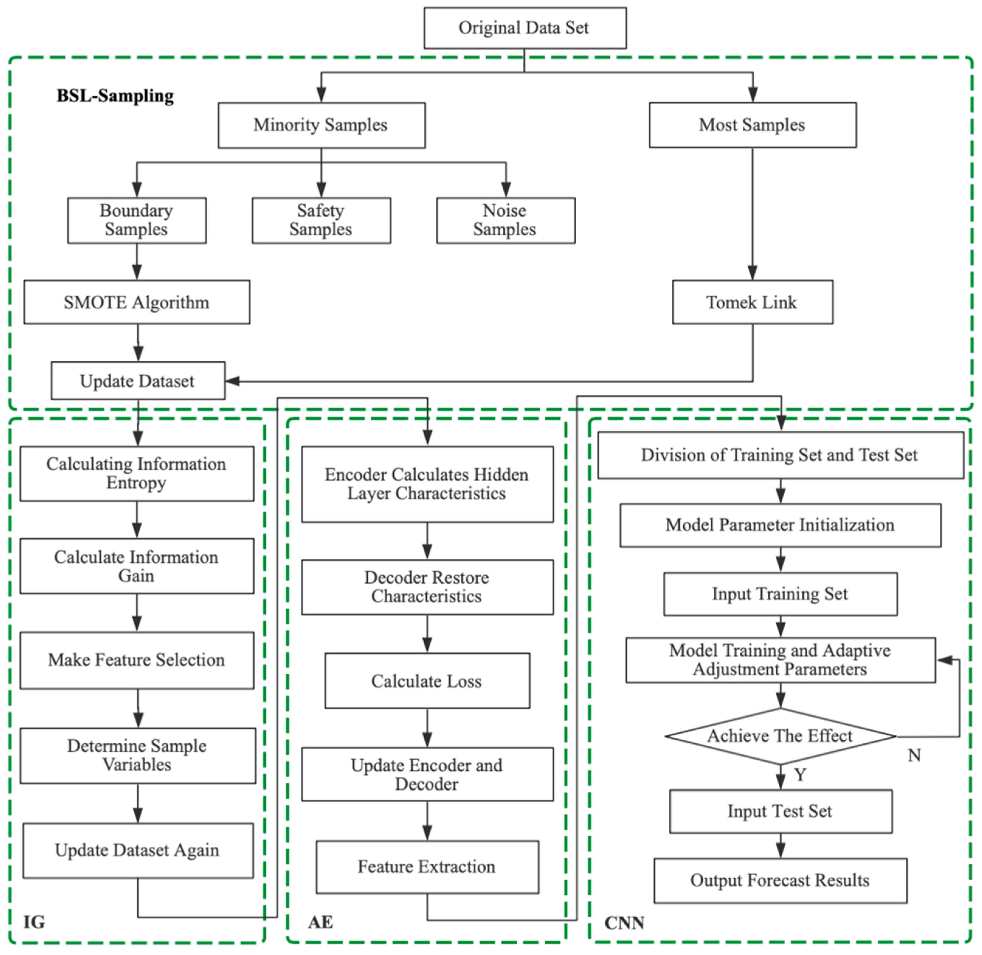
3.3.3. AE-CNN Sports Risk Prediction Algorithm Flow

To solve the problems of difficult extraction of motion risk features and insufficient prediction accuracy, this chapter combines AE and CNN to build a motion risk prediction model, aiming to take advantage of self-encoders and convolutional neural networks to improve the performance and efficiency of deep learning models in motion risk prediction. AE-CNN contains a self-encoder module for feature extraction and dimensionality reduction, and the self-encoder can completely express motion. The AE-CNN includes a self-encoder module for feature extraction and dimensionality reduction, which is able to fully represent the features of the risk and can improve the efficient use of raw data. The self-encoder module consists of an encoder and a decoder, where the encoder converts the input data into a low-dimensional dense representation and the decoder converts the low-dimensional representation back to the original data. The learning process of the self-encoder is unsupervised, which can make full use of the information in the unlabeled data. Afterwards, the output of the self-encoder is fed into a convolutional neural network for classification prediction. The convolutional neural network consists of a convolutional layer, a pooling layer, and a fully connected layer, which can automatically learn a high-dimensional nonlinear feature representation and accomplish causal inference between risk features and risk factors. In this process, the feature extractor of the self-encoder module can reduce the noise and redundant information of the input data and improve the performance and efficiency of the convolutional neural network. Finally, AE-CNN achieves end-to-end learning by using feature transfer between the two modules. The self-encoder part extracts the features of the input data, and the convolutional neural network uses these features to further improve performance. The whole AE-CNN model can be trained through supervised or unsupervised learning. This model can effectively extract feature information and better solve the problem that traditional models are difficult to handle for high-dimensional and nonlinear data.

The motion risk prediction model based on auto-coding and convolutional neural networks proposed in this chapter consists of four modules: the data set equalization module, feature selection module, self-encoder feature extraction module, and convolutional neural network prediction module. Specifically, firstly, the BSL sampling technique is applied to perform the data set equalization operation and update the data set. Secondly, the feature selection of the equalized dataset is performed by the IG method to determine the sample variables. Then AE is used to perform feature dimensionality reduction and hidden representation extraction, which are used as the set of sensitive features that can reflect the risk category as the input of CNN. Finally, the delineated training set is used to learn the structure of the CNN, and the directed relationship between risk features and risk types is obtained to perform the prediction of motion risk categories and derive the corresponding risk categories. In the AE-CNN model, the convolutional neural network can also avoid overfitting by using operations such as pooling and dropout. To improve the prediction accuracy of the AE-CNN model, feature selection and fusion techniques are applied to the model. Specifically, features that have a better correlation to the target variables are selected from a large amount of personal health data using feature selection techniques. Through feature fusion techniques, data features from different modalities are combined to improve the accuracy and robustness of feature characterization. In summary, the AE-CNN model combines advanced technologies such as self-encoder and convolutional neural networks, which can improve the accuracy and generalization ability of the exercise risk prediction model and provide more accurate and personalized preventive measures and intervention suggestions for exercisers. The specific algorithm flow of the AE-CNN model is shown in Figure 4.

4. Results and Discussion

4.1. Model Evaluation Indicators

Classification is a common task in machine learning. When evaluating the effectiveness of classification models, it is often necessary to use a variety of different evaluation indicators to evaluate multiple aspects. This research mainly uses the following evaluation indicators to evaluate the performance of the algorithm.

(1)

Accuracy (ACC)

The calculation formula is as follows:

$$\mathrm{A}\mathrm{C}\mathrm{C}=\frac{\mathrm{T}\mathrm{P}+\mathrm{F}\mathrm{N}}{\mathrm{T}\mathrm{P}+\mathrm{T}\mathrm{N}+\mathrm{F}\mathrm{P}+\mathrm{F}\mathrm{N}}$$

(11)

where TP, TN, FP, and FN represent true positive, true negative, false positive, and false negative, respectively.

(2)

Recall

The calculation formula is as follows:

$$\mathrm{R}\mathrm{e}\mathrm{c}\mathrm{a}\mathrm{l}\mathrm{l}=\frac{\mathrm{T}\mathrm{P}}{\mathrm{T}\mathrm{P}+\mathrm{F}\mathrm{N}}$$

(12)

(3)

Specificity

The calculation formula is as follows:

$$\mathrm{S}\mathrm{p}\mathrm{e}\mathrm{c}\mathrm{i}\mathrm{f}\mathrm{i}\mathrm{c}\mathrm{i}\mathrm{t}\mathrm{y}=\frac{\mathrm{T}\mathrm{N}}{\mathrm{T}\mathrm{N}+\mathrm{F}\mathrm{P}}$$

(13)

(4)

Precision

The calculation formula is as follows:

$$\mathrm{P}\mathrm{r}\mathrm{e}\mathrm{c}\mathrm{i}\mathrm{s}\mathrm{i}\mathrm{o}\mathrm{n}=\frac{\mathrm{T}\mathrm{P}}{\mathrm{T}\mathrm{P}+\mathrm{F}\mathrm{P}}$$

(14)

(5)

F1-score

The calculation formula is as follows:

$$\mathrm{F}1=\frac{2\times \mathrm{R}\mathrm{e}\mathrm{c}\mathrm{a}\mathrm{l}\mathrm{l}\times \mathrm{P}\mathrm{r}\mathrm{e}\mathrm{c}\mathrm{i}\mathrm{s}\mathrm{i}\mathrm{o}\mathrm{n}}{\mathrm{R}\mathrm{e}\mathrm{c}\mathrm{a}\mathrm{l}\mathrm{l}+\mathrm{P}\mathrm{r}\mathrm{e}\mathrm{c}\mathrm{i}\mathrm{s}\mathrm{i}\mathrm{o}\mathrm{n}}$$

(15)

4.2. Data Set Introduction

The data used in this experiment are simulation data under various sports conditions, which are mainly used to verify the feasibility of the model algorithm. The generation process is to establish the corresponding relationship function (such as height and weight, circumference, obesity, basic heart rate, etc.) according to the corresponding relationship between user attributes and then add various possible disturbance factors through Gaussian perturbation to make the data more reasonable. The data set includes 13,525 athletes, and each athlete corresponds to 25 columns of characteristics. The first 24 columns are risk factor data, including age, gender, height, weight, body shape, medical history, cognitive impairment, quality index, sports events, sports frequency, sports time, sports intensity, endurance, strength, flexibility, balance, sports field, and sports equipment. The 25th column is the label data, i.e., risk category, including fall, fracture, joint sprain, tissue contusion, shock, and sudden death.

4.3. Analysis of Experimental Results

The algorithm experiment environment in this chapter uses the Python 3.6 programming language in the open-source deep learning tool TensorFlow to achieve the preprocessing operation of the sports risk data set as well as the construction and analysis of the sports risk prediction model. During the modeling process, machine learning libraries such as pandas, numpy, matplotlib, and Keras are used.

4.3.1. Sports Risk Prediction Results Based on AE-CNN

After IG, the features are reduced to 10, and the reduced dimension data set is divided into a training set and a verification set with a ratio of 8:2. 2705 samples are randomly selected as a test set to test the model. In the convolution neural network constructed, the size of the convolution core of the convolution layer is 2 × 1. The nonlinear activation function ReLu is adopted as the activation function. To avoid overfitting and improve the generalization ability of the model, dropout is added after the maximum pool layer, and the dropout loss rate is set to 0.3. The output layer is the full connection layer, the output is 6, the activation function is SoftMax, the optimizer selects Adam, the learning rate is set to 0.001, the loss function is set to cross-entropy error, and the number of iterations is set to 50 to train the model.

In order to prove the feasibility and effectiveness of this method, the CNN with AE processing as an input feature, namely AE-CNN, is compared with the CNN with the original feature as input. The results are shown in Figure 5. This shows that the AE-CNN model used in this paper has a better prediction effect.

4.3.2. Comparison Experiment

The algorithm used in this paper is compared with the traditional machine learning classification algorithms: Bayesian network (BN), KNN, support vector machine (SVM), and multilayer perception machine (MLP). The experimental comparison results are shown in

Table 3. Comparison of prediction effects of different classification algorithms.

Methods	ACC	Recall	Specificity	F1-Score	Precision
BN	0.7837 ± 1.61	0.7344 ± 1.64	0.7956 ± 1.48	0.7660 ± 1.83	0.6973 ± 1.75
KNN	0.7581 ± 2.34	0.8166 ± 1.05	0.7836 ± 1.74	0.8420 ± 1.06	0.7562 ± 0.85
SVM	0.8327 ± 0.81	0.7490 ± 0.85	0.8864 ± 0.92	0.8310 ± 0.94	0.7817 ± 0.86
MLP	0.8763 ± 1.05	0.8650 ± 1.38	0.8800 ± 1.01	0.8420 ± 1.05	0.8084 ± 1.06
AE-CNN	0.9334 ± 0.21	0.9325 ± 0.26	0.9370 ± 0.30	0.9297 ± 0.19	0.9366 ± 0.20

.

According to the experimental results in Table 3, the classification effect of the naive Bayesian algorithm and the K nearest neighbor algorithm is poor. The reason is that the algorithm principle of Naive Bayes is to give the output category through a priori and a posteriori probabilities. Once there is a high correlation between sample data, the classification effect will be poor. The core idea of the K nearest neighbor algorithm is to use the principle of proximity in the feature space for classification, but most of the risk feature data are discrete, lacking correlation between features, so the prediction accuracy is insufficient. Support vector machines and multi-layer perceptrons perform well. A support vector machine maps low-dimensional linear indivisible samples to high-dimensional separable space through various kernel functions. However, with the increasing amount of data, the mapping dimension of kernel functions in support vector machines will continue to increase, which affects the timeliness of the prediction model. Therefore, this model is not suitable for processing large-scale sample data. With the improvement in computing power of computer hardware, the multilayer perceptron performs well in algorithm performance, but a single multilayer perceptron cannot compress discrete high-dimensional features in advance when dealing with a high-dimensional sparse matrix, thus increasing the computational load of model training, so the prediction effect will be affected. The experimental results show that the AE-CNN algorithm used in this paper is superior to several traditional classification algorithms, which shows that the algorithm model in this paper is effective, can better deal with the sports risk prediction problem, and has a stronger ability to extract discrete data features. The extracted features are more robust, and the model is more generalized and accurate.

5. Conclusions

(1)

This paper combines AE and CNN to analyze and predict the characteristics of sports risk categories. The algorithm model can effectively extract the characteristics of sports risk, analyze the risk factors, and use AE to extract the characteristics, thus completing the efficient representation of sports risk.

(2)

The algorithm uses CNN to realize the prediction of sports risk categories. Considering the size and characteristics of the dataset, this paper adopts the topology structure of a double convolution layer and a double pool layer to complete the CNN modeling.

(3)

The comparison of prediction results of different classification algorithms, that is, the verification of model evaluation indicators, shows that this model can effectively predict sports risk categories, reduce the impact of redundant data, and effectively improve the accuracy of sports risk prediction.

(4)

At present, the research on the application of machine learning in the field of sports risk is still in its infancy, and there are still many problems due to the great differences in various aspects of research in this field at home and abroad. The application of machine learning in the field of sports injury still has great development potential, and more research on its model algorithm and calculation is needed.

References

1. Quatman, C.E.; Quatman, C.C.; Hewett, T.E. Prediction and prevention of musculoskeletal injury: A paradigm shift in methodology. Br. J. Sport. Med. 2009, 43, 1100–1107. [Google Scholar] [CrossRef] [PubMed]
2. Meeuwisse; Willem, H.; Tyreman; Hugh; Hagel; Brent. A dynamic model of etiology in sport injury: The recursive nature of risk and causation. Clin. J. Sport Med. 2007, 17, 215–219. [Google Scholar] [CrossRef]
3. Talukder, H.M.; Stowell, T.B. Pneumatic hammer in an externally pressurized orifice-compensated air journal bearing. Tribol. Int. 2003, 36, 585–591. [Google Scholar] [CrossRef]
4. Luu, B.C.; Wright, A.L.; Haeberle, H.S.; Karnuta, J.M.; Schickendantz, M.S.; Makhni, E.C. Machine learning outperforms logistic regression analysis to predict next season NHL player injury: An analysis of 2322 players from 2007 to 2017. Orthop. J. Sport. Med. 2020, 8. [Google Scholar] [CrossRef]
5. Jauhiainen, S.; Kauppi, J.P.; Leppnen, M.; Pasanen, K.; Parkkari, J.; Vasankari, T. New machine learning approach for detection of injury risk factors in young team sport athletes. Int. J. Sport. Med. 2021, 42, 175–182. [Google Scholar] [CrossRef]
6. Rossi, A.; Pappalardo, L.; Cintia, P.; Iaia, M.; Fernandez, J.; Medina, D. Effective injury forecasting in soccer with GPS training data and machine learning. PLoS ONE 2018, 13, e0201264. [Google Scholar] [CrossRef] [PubMed] [Green Version]
7. Gao, X.L.; Shi, Y.J.; Yang, H.J. A study on the prediction of injury risk of Chinese rugby players by multilayer perceptron neural network model. In Proceedings of the 11th National Sports Science Conference, Nanjing, China, 1–3 November 2019; pp. 5797–5799. [Google Scholar] [CrossRef]
8. Rommers, N.; Roland, R.; Verhagen, E.; Vandecasteele, F.; Verstockt, S.; Vaeyens, R. A machine learning approach to assess injury risk in elite youth football players. Med. Sci. Sport. Exerc. 2020, 8, 1. [Google Scholar] [CrossRef]
9. Orlando, A. AI for Sport in the EU Legal Framework. In Proceedings of the 2022 IEEE International Workshop on Sport, Technology and Research (STAR), Cavalese, Italy, 6–8 July 2022; pp. 100–105. [Google Scholar] [CrossRef]
10. McManus, K.; Greene, B.R.; Ader, L.G.M.; Caulfield, B. Development of Data-Driven Metrics for Balance Impairment and Fall Risk Assessment in Older Adults. IEEE Trans. Biomed. Eng. 2022, 69, 2324–2332. [Google Scholar] [CrossRef]
11. Ruddy, J.D.; Shield, A.J.; Maniar, N.; Williams, M.D.; Duhig, S.; Timmins, R.G.; Hickey, J.; Bourne, M.N.; Opar, D.A. Predictive modeling of hamstring strain injuries in elite Australian footballers. Med. Sci. Sport. Exerc. 2018, 50, 906–914. [Google Scholar] [CrossRef] [Green Version]
12. Ayala, F.; López-Valenciano, A.; Gámez Martín, J.A.; Mark, D.S.C.; Vera-Garcia, F.; García-Vaquero, M. A preventive model for hamstring injuries in professional soccer: Learning Algorithms. Int. J. Sport. Med. 2019, 40, 344. [Google Scholar] [CrossRef] [PubMed]
13. Claudino, J.G.; Capanema, D.D.O.; Souza, T.V.D.; Julio, C.S.; Nassis, G.P. Current approaches to the use of artificial intelligence for injury risk assessment and performance prediction in team sports: A systematic review. Sport. Med. 2019, 5, 28. [Google Scholar] [CrossRef] [PubMed] [Green Version]
14. Li, C.; Zhou, T.; Guo, Q.; Cui, H.L. Compressive Beamforming Based on Multiconstraint Bayesian Framework. IEEE Trans. Geosci. Remote Sens. 2021, 59, 9209–9223. [Google Scholar] [CrossRef]
15. Ciprian, C.; Masychev, K.; Ravan, M.; Reilly, J.P.; Maccrimmon, D. A Machine Learning Approach Using Effective Connectivity to Predict Response to Clozapine Treatment. IEEE Trans. Neural Syst. Rehabil. Eng. 2020, 28, 2598–2607. [Google Scholar] [CrossRef]
16. Berta, M.; Renes, J.M.; Wilde, M.M. Identifying the Information Gain of a Quantum Measurement. IEEE Trans. Inf. Theory 2014, 60, 7987–8006. [Google Scholar] [CrossRef] [Green Version]
17. Gao, H.; Zhang, X.; Wen, J.; Yuan, J.; Fang, Y. Autonomous Indoor Exploration via Polygon Map Construction and Graph-Based SLAM Using Directional Endpoint Features. IEEE Trans. Autom. Sci. Eng. 2019, 16, 1531–1542. [Google Scholar] [CrossRef]
18. Si, W.; Fu, C.; Yuan, P. An Integrated Sensor with AE and UHF Methods for Partial Discharges Detection in Transformers Based on Oil Valve. IEEE Sens. Lett. 2019, 3, 1–3. [Google Scholar] [CrossRef]
19. Roy, S.K.; Krishna, G.; Dubey, S.R.; Chaudhuri, B.B. HybridSN: Exploring 3-D–2-D CNN Feature Hierarchy for Hyperspectral Image Classification. IEEE Geosci. Remote Sens. Lett. 2020, 17, 277–281. [Google Scholar] [CrossRef] [Green Version]
20. Ahmed, S.; Kim, W.; Park, J.; Cho, S.H. Radar-Based Air-Writing Gesture Recognition Using a Novel Multistream CNN Approach. IEEE Internet Things J. 2022, 9, 23869–23880. [Google Scholar] [CrossRef]
21. Karlsson, K.; Hendeby, G. Speed estimation from vibrations using a deep learning CNN approach. IEEE Sens. Lett. 2021, 5, 1–4. [Google Scholar] [CrossRef]
22. Srivastava, N.; Hinton, G.; Krizhevsky, A.; Sutskever, I.; Salakhutdinov, R. Dropout: A simple way to prevent neural networks from overfitting. J. Mach. Learn. Res. 2014, 15, 1929–1958. [Google Scholar]
23. Huang, Y.Q.; Li, Y.R.; Gui, Y.H. Machine learning: A new way to prevent sports injury. Fujian Sport. Sci. Technol. 2021, 40, 12–18. [Google Scholar]
24. Zhang, Y.; Luo, L. Thoughts on the classification system of sports risk. J. Sport. Adult Educ. 2012, 28, 20–21. [Google Scholar] [CrossRef]
25. Blanch, P.; Gabbett, T.J. Has the athlete trained enough to return to play safely? The acute:chronic workload ratio permits clinicians to quantify a player’s risk of subsequent injury. Br. J. Sport. Med. 2016, 50, 471–475. [Google Scholar] [CrossRef] [PubMed]
26. Yza, B.; Sl, A.; Tx, C.; Tao, W.C. Application of convolutional neural network in random structural damage identification. Structures 2021, 29, 570–576. [Google Scholar] [CrossRef]
Figure 1. Model framework.
Applsci 13 07839 g001
Figure 2. Importance of sports risk characteristics based on IG.
Applsci 13 07839 g002
Figure 3. Structure of AE.
Applsci 13 07839 g003
Figure 4. Flow chart of AE-CNN model prediction.
Applsci 13 07839 g004
Figure 5. (a) Comparison curve of accuracy between CNN and AE-CNN; (b) comparison curve of loss between CNN and AE-CNN.
Applsci 13 07839 g005