Abstract
Dementias that develop in older people test the limits of modern medicine. As far as dementia in older people goes, Alzheimer’s disease (AD) is by far the most prevalent form. For over fifty years, medical and exclusion criteria were used to diagnose AD, with an accuracy of only 85 per cent. This did not allow for a correct diagnosis, which could be validated only through postmortem examination. Diagnosis of AD can be sped up, and the course of the disease can be predicted by applying machine learning (ML) techniques to Magnetic Resonance Imaging (MRI) techniques. Dementia in specific seniors could be predicted using data from AD screenings and ML classifiers. Classifier performance for AD subjects can be enhanced by including demographic information from the MRI and the patient’s preexisting conditions. In this article, we have used the Alzheimer’s Disease Neuroimaging Initiative (ADNI) dataset. In addition, we proposed a framework for the AD/non-AD classification of dementia patients using longitudinal brain MRI features and Deep Belief Network (DBN) trained with the Mayfly Optimization Algorithm (MOA). An IoT-enabled portable MR imaging device is used to capture real-time patient MR images and identify anomalies in MRI scans to detect and classify AD. Our experiments validate that the predictive power of all models is greatly enhanced by including early information about comorbidities and medication characteristics. The random forest model outclasses other models in terms of precision. This research is the first to examine how AD forecasting can benefit from using multimodal time-series data. The ability to distinguish between healthy and diseased patients is demonstrated by the DBN-MOA accuracy of 97.456%, f-Score of 93.187 %, recall of 95.789 % and precision of 94.621% achieved by the proposed technique. The experimental results of this research demonstrate the efficacy, superiority, and applicability of the DBN-MOA algorithm developed for the purpose of AD diagnosis.
1. Introduction
When ranked by prevalence, AD ranks third in the US, behind cardiovascular disease and cancer, and is the sixth leading cause of death worldwide [1]. The entorhinal cortex, the hippocampus neocortex, and other brain regions are highly susceptible to neuronal cell death, neurofibrillary tangles, and senile plaques that characterize AD. The number of people living with dementia is expected to rise from its current 75.6 million to 135.5 million by 2050 [2].
For the past fifty years, studies on AD have predicated on including and excluding specific clinical factors. Clinical criteria are only 85% accurate in detecting AD, so a detailed examination is necessary for a definitive diagnosis [3]. The role of instrumental tests in clinical diagnosis such as detecting cerebral atrophy on a brain scan or measuring the concentration of specific proteins in a patient’s blood has grown over time. Quantitative evaluation is intrinsically linked to the creation of novel neuroimaging techniques.
Dementia can be detected in its earliest stages with the help of neuroimaging techniques developed by the ADNI. Recent advances in neuroimaging techniques, such as MRI, have allowed researchers to identify and present novel molecular and structural biomarkers for AD. Clinical trials have demonstrated that the diagnostic accuracy of neuroimaging techniques like MRI is improved. It has been speculated that MRI can detect abnormalities in brain morphology related to mild cognitive impairment (MCI) and thus accurately predict the progression from MCI to AD. The aim is to identify structural and molecular hallmarks of AD. Clinical studies have demonstrated increased diagnostic accuracy of neuroimaging modalities like MRI [4]. It has been hypothesized that MRI can reliably predict whether or not a person with MCI will develop AD by detecting the abnormalities in brain morphology that are characteristic of MCI.
There has also been a call for research into “multimodal biological markers,” which may aid in the initial diagnosis of AD [5]. Electroencephalogram (EEG) data, neuropsychological data, demographic data, APOE4 genotype data, and MRI information were used to train the ML classifier by Gaubert et al. [6]. The model is educated to recognize the onset of AD and its telltale signs, including amyloid plaques and neuronal degeneration. After five years, EEG can predict neurodegenerative diseases, just as amyloid accumulation and prodromal diseases can be predicted with psychographic and MRI data. This study confirmed previous findings that used ML techniques to predict AD onset successfully. Being able to form opinions rapidly is the end result [7]. Several supervised Ensemble methods were compared and analyzed for their potential use in the classification of AD [8]. Some claims of improved classification accuracy and specificity have been made for boosting models [9], like the generalized boosting model and the gradient boosting machines (GBM).
Using ML expertise and the patient’s medical records, dementia can also be predicted. Dementia onset prediction using AD patient records over two years using a gradient boosting model (light GBM) was also proposed [10]. In the end, we got an accuracy rate of 87%. The use of recurrent neural networks (RNN) to simulate the development of AD was also proposed [11]. Data assertion and regression methods were used to evaluate it against an alternative RNN model. As a result, when training on unlabeled data, accuracy reached 74%. The inter-data relationship between MRI demographic data and AD can also be learned. Studies have shown that random forest (RF) models perform better than other models, including support vector machine (SVM) models, when using this technique [12]. Deep learning models can forecast the advancement from MCI to AD [13]. Since deep learning models benefit from more information, pre-processing unlabeled data is a good idea [14]. Several studies [15] have shown promise in using deep learning to diagnose AD and detect symptoms. With the help of a deep learning model that is both precise and thorough in identifying the first signs of AD, the disease could be diagnosed and treated much sooner.
Discretizing MRI data and handling outliers effectively can improve ML classification accuracy. Reportedly, people with dementia can be accurately categorized using supervised models in conjunction with feature selection [16]. In another investigation [17], multifactor affiliation analysis was used to categorize patients according to the interrelationships of features. This method excels beyond classification trees and generic distribution zones in classifying patients and efficiency. These methods failed to show how crucial it is to use data-centric ML techniques and embrace model-boosting knowledge to turn inefficient learners into efficient ones and enhance model performance [18]. IoT applications are spreading throughout the medical industry [19]. IoT can be used to sense real-time patient data and other environmental detail and can be sent for further processing [20]. It helps in fast data processing, relief from manual work and avoiding mistakes while digitizing the records [21]. IoT-enabled portable MR imaging device captures real-time patient MR images and identifies anomalies in MRI scans for detecting and classifying AD [22].
The more recent algorithm is known as mayfly optimization (MOA.) This algorithm could be used to identify male and female mayflies in a group. Each one of them updates in its own special way. If a person’s current position was extremely far from the best contender or the historically best trajectories, their progress toward the best position slowed in the MO algorithm’s initial iteration. It is easy to see how such actions could immediately slow the rate of convergence. To boost the efficiency of MOA algorithms, we suggest rewriting the updating equations that have been applied throughout this paper.
In this paper, we make significant advancements over previous work in both the accuracy with which DBN can classify the status of a patient and its ability to deal with voice features. DBN use many processing layers to model higher-level abstractions in complex data structures. Weighted connections link the processing layers together, but the layers themselves are isolated. It allows us to view it as a generative graphical model with many hidden nested units, similar to the structure of a tree. These networks can only learn as much as their trainers allow when given supervised and unsupervised training.
The current survey’s contributions are summarized as follows:
- Evaluate how well the current model can foresee the development of AD using the ADNI database.
- In addition, we proposed a framework for AD/non-AD classification of dementia subjects using longitudinal brain MRI features and DBN with an MOA.
- In contrast to the current literature, our DBN-MOA models are optimized by considering a wide range of low-cost time-series features, such as patients’ comorbidities, cognitive scores, medication histories, and demographics.
The following topics make up the study’s subsections: In Section 2, we provided a review of the recent related works. Part III, look at the fundamentals of DBN and proposed a DBN- MOA approach for Alzheimer detection with detailed algorithms. Section 4 discusses the proposed model and compared the output results with the similar approaches provided in other studies. The paper’s final Section 5 discusses the proposed model’s implications and directions for future research.
2. Literature Survey
Cao et al. [23] created a new optimization strategy to enhance the mixed-norm regularised formulation. When tested on the ADNI datasets, cognitive measurements using multimodality or single MRI modality data showed enhanced classification performance and a condensed set of AD biomarkers was produced. The use of full 3D image data for differential diagnosis may call for larger training sets. Artificial intelligence algorithms that have been trained on large datasets may be more useful than CAD when applied to medical images. Because of this, the current state of AI-based medical image analysis is limited. When presented with novel images captured under extremely diverse conditions, artificial intelligence techniques quickly degrade from their stellar performance in a lab setting with uniform imaging protocols.
Nawaz et al. [24] compared three models to determine which one was the most accurate. The first model involves preparing an image for classification using SVM, KNN, or Random Forest by applying manually created features. The second model employs a convolutional neural network (CNN) deep learning model with cleaned and prepped data. AlexNet is used to extract deep features in SVM, k-nearest neighbor, and Random Forest. SVM classifiers performed best for the deep features-based model. K-nearest neighbor algorithms have an accuracy of 57.32 per cent, whereas SVM have an accuracy of 95.21 per cent, and random forest algorithms have an accuracy of 93.9 per cent.
Feng et al. [25] suggested a new deep learning architecture that combines 3D-enhanced CNN with stacked bidirectional RNN (SBi-RNN CNNs). Extraction of deep feature depiction from MRI and PET images is the focus of this paper, which argues for the use of a simple 3D-CNN framework. Using SBi-RNN enhanced the functionality of locally deep cascaded and compressed features. Several trials were conducted on the ADNI dataset to evaluate the recommended structure’s efficacy. Analyzing the proposed architecture against the NC cohort revealed an average precision of 64.47 per cent for sMCI, 94.29% for AD, and 84.66% for pMCI.
Jenugopalan et al. [26] combined data from various sources, including MRI scans, to better comprehend AD. Every CNN was trained with every type of data. Then, an integrated classification was carried out using random forests, SVMs, trees, and k-nearest neighbours. Evidence herein shows that combining data from multiple sources improves prediction accuracy. The small size of its dataset hinders the current study. The survey is presented in Table 1.

Table 1.
Survey of existing literature on AD detection.
To reveal the dementia and mild cognitive deficiency, Wang et al. [35] suggest a set of densely linked 3D convolutional networks (3D-DenseNets) using a probability-based fusion technique (MCI). In 3D-DenseNets, all of the layers are interconnected, which speeds up the gradient propagation. MRI scans are used as the training data. The results of DenseNets are also calculated with the help of a softmax function. The classification accuracy of DenseNets was 97.52 per cent when tested on the ADNI dataset.
With the help of longitudinal data collected before the testing period and a random forest regression algorithm, Huanget et al. [36] could predict the subjects’ cognitive scores. Precise, constant, and medically instinctive models can be obtained by analyzing multimodal time series data with the right ML models. The usage of multimodal time series data is likely to improve model performance when attempting to predict the progression of AD.
Kundaram et al. [37] pre-processed the images by resizing them to 255 in brightness and contrast. To train and categorize diseases, CNN models are used [38,39]. The images were divided into three groups (AD, MCI, and NC) that used 9540 images in the model-training process. The CNN model consists of four ReLU activation layers, three max-pooling layers, and three convolutional layers. Various optimizers were implemented, including Adam, S.G.D., Adadelta, Nadam, Adagrad, and Rmsprop. Adagrad outperforms competing optimizers in the proposed framework by achieving higher precision at a lower cost. The proposed model performed at a 98.57 per cent accuracy on the ADNI dataset.
Mishra et al. [40] have contributed to this field. It is suggested that deep learning models be developed to facilitate automated feature extraction from imaging data. Scientists are working to develop a deep-learning model for reliable disease diagnosis. Many medical imaging modalities, from CT and MRI scans to x-rays and ultrasounds, have benefited greatly from applying deep learning models [41]. The most recent proposal for a cutting-edge ML system to automatically and swiftly diagnose AD was made by Zhang et al. [42]. The binary classifier used for this study was trained with 196 subjects’ volumetric MRI data. The training procedure benefited from this information. These data were utilized in a number of ways during the training process.
Korolev et al. [43] demonstrated comparable performance. Both the residual network and the plain 3D CNN architectures showed very long depth and complex behavior when trained on 3D structural MRI. Their results were subpar in comparison to what was hoped for. In order to introduce a CNN architecture, Ding et al. [44] first used an Inception v3 network trained on 90% of the ADNI data and testing 10%. Scans for pets using fluorine-18 fluorodeoxyglucose are analyzed using grid processing. Images obtained from the ADNI data set. Using the Otsu threshold, the brain’s voxels were assigned labels. Adam’s learning ratio was 0.0001, and the batch size was 8. The models were trained using 90% of the availabel data (1921 images). This data set contains information from three distinct demographics (AD, MCI, and no disease). Despite its high sensitivity, the proposed structure has a low level of specificity (only 82%).
It was proposed by Beheshti et al. [45] that a system could be developed to detect AD using feature position and structural MRI data. The created framework is comprised of multiple actionable steps: (i) Differentiating the GM of AD patients from that of HCs requires I a voxel-based morphometry procedure, (ii) the creation of raw features based on the voxel frequency components of the volumes of interest, and (iii) the ranking of the raw features using a seven-feature ranking technique. The most distinguishing feature between HC and AD groups is the vector size that produces the smallest classification error. A classification is made using a SVM in (iv). Extensive research has demonstrated that incorporating a data fusion technique into feature ranking approaches enhances their ability to classify input data correctly. The accuracy of the developed framework for diagnosing AD was 92.48 per cent when trained on the ADNI dataset.
3. Proposed System
A block diagram depicting the proposed DBN-MOA has been given in Figure 1 below. The figure elucidates the data collection and pre-processing steps in detail. In order to test hypotheses and assess results, data collection entails amassing and measuring relevant information on relevant variables in a predetermined, systematic manner. It is a decisive in the research process because it supports the researcher in making sense of the availabel data and determine that how it can help in progression of the project forward. The term “data pre-processing” refers to any action taken on raw data before it undergoes further processing. It is a crucial first step in data mining and has been for a long time.
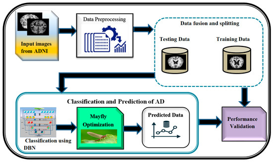
Figure 1.
Proposed diagram of DBN-MOA.
The pre-processed data is then fused and split; data fusion is the process of combining information from different sources to create accurate, complete, and consistent data about a single entity, and data splitting is the reverse of that procedure. Feature-level, Low-level, and decision-level data fusion are the three main types. Separating a dataset into two subsets, or “splits,” is common in cross-validation analyses. The data is split in two, with one half used to build a predictive model and the other half for testing. The DBN-MAO algorithm is then used to optimize the classification of the data. Finally, the accuracy of the predicted data is confirmed through independent validation, demonstrating the method’s superiority over its competitors.
3.1. Dataset Collection
We sourced all of our information from the ADNI dataset [46]. ADNI is an invaluable resource for researchers [47]. A total of 416 people were included in this cross-sectional dataset. The ages of these participants range from 18 to 96 years. Three or four independent T1-weighted MRI scans are acquired in a single session for each subject. The sample images from the ADNI dataset have been presented in Figure 2.
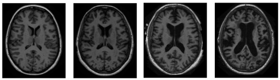
Figure 2.
Sample pictures of an AD patient from the ADNI dataset.
Both sexes are represented, and everyone is dominantly right-handed. From very mild to moderate AD, 100 of the 416 subjects aged 60+ have been diagnosed. A reliability data set, with images from the follow-up appointment within 90 days, is also included for 20 people without dementia.
3.2. Data Pre-Processing
The relationship between cognitive tests, medication, and mental health is depicted graphically in Figure 3. We have investigated the utility of multimodal time-series data in making prognoses about the course of AD.
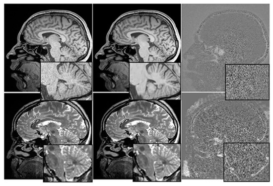
Figure 3.
Before and After Denoising.
Each patient is represented by four rows in each of the four time-series representations, with each row containing information from a single visit. The ADNI compiles attendance statistics once every six months. Researchers on the ADNI project gathered massive amounts of information over the course of more than a decade.
We have used T1-weighted MRI images acquired from a cohort of 100 patients diagnosed with AD and 100 age-matched healthy controls. The MRI images having a resolution of 1 mm × 1 mm × 1 mm and dimensions of 256 × 256 × 160. The intensity values of each pixel in the MRI images ranged from 0 to 255.
Before training the Mayfly optimization algorithm, the MRI images were pre-processed by applying skull stripping, intensity normalization, and spatial normalization using the SPM12 toolbox. The images segmented into grey matter, white matter, and cerebrospinal fluid using the FSL software.
To train the algorithm, leave-one-out cross-validation approach has been used where one patient was left out for testing, and the remaining 199 patients for training. The input to the algorithm consisted of the segmented grey matter images, which were resized to 128 × 128 × 80 to reduce the computational burden.
By providing this level of detail about the input data, the authors can help readers better understand the characteristics of the MRI images used in the study and how they may have influenced the results. This information can also be useful for other researchers who want to reproduce the study or compare it with other studies that use similar input data.
Data Labelling
Our sample size was also set after we finished pre-processing and labelled our data for binary classification. Since we are engaging in binary classification, each record in the dataset has been either given a zero or a one for the Clinical Dementia Ratio (CDR). Keep in mind that a CDR of 0 denotes perfect health (i.e., no signs of dementia), and a CDR of 1 indicates severe Alzheimer’s (i.e., demented). To date, 28 patients have been diagnosed with CDR 1. We used a total of 28 patients with AD and 28 controls to make our classifications. We have two pictures of each patient. We then randomly split the dataset into halves, creating an 8:2 split. It means that eighty per cent of the data is used for training and twenty per cent for testing. The proposed DBN-MOA method diagram is depicted in Figure 1.
3.3. Data Fusion and Splitting
The combined dataset from the five modalities is then used for either training (representing 90% of the data) or testing (representing 10% of the data). After being fine-tuned and trained on the training set, all ML models are then evaluated on the test set, which they have never seen before.
3.4. Deep Belief Network
A Deep Belief Network (DBN) is a type of generative model that utilizes multiple processing layers to capture complex structures and abstractions in data. It consists of a series of individually trained Restricted Boltzmann Machines (RBMs) stacked on top of each other. The RBMs in a DBN are trained in an unsupervised manner, where the training process begins with an unsupervised stage.
In a DBN, there are typically two processing layers in each of the RBMs, referred to as the “visible” layer and the “hidden” layer. The visible layer represents the observable entities or features of the data, while the hidden layer captures latent or hidden representations. The units within the same layer of an RBM do not have direct connections to each other. Instead, the interconnectedness between layers allows for the construction and reconstruction processes.
The training of a DBN involves iteratively training each RBM in a layer-wise manner. The first RBM is trained using the visible layer as input, and its hidden layer activations become the visible layer for the next RBM. This process continues until all RBMs are trained. This layer-wise pretraining helps to fix problems that can occur when the network is initially set up with untrained, arbitrary connection weights. Using unsupervised learning techniques, generative stochastic neural networks can be learned from probability models. The RBM’s network has two distinct processing levels, labelled “visible” and “hidden” in Figure 4. The units within the same layer have no connection to one another, but the construction and reconstruction processes are made possible by the interconnectedness of these layers. A large quantity of observable entities make up the network’s visible layer (v), which is trained on the unlabeled pattern structures fed into it, and a large number of unseen entities Unseen nodes in the network have binary values, receive information from the seen nodes, and are able to reconstruct the patterns (h).
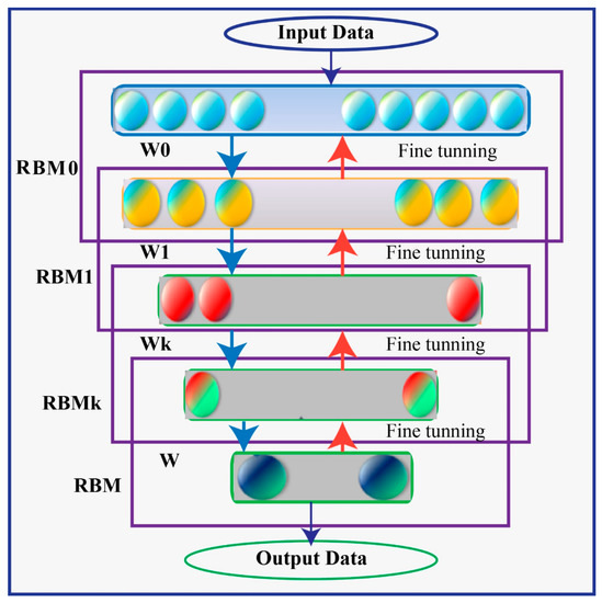
Figure 4.
Deep Belief Network (DBN) Architecture.
All the obvious nodes talk to all the obvious nodes as a symmetric two-way matrix of weight , in addition to the biases and that are already there.
where represents the dispersion of the Gaussian noise in the ith visible dimension.
The learning process may become more challenging if both the exposed and concealed units are Gaussians. The standard deviations of the assumed noise levels are used to calculate the coefficients of the quadratic “containment” terms that keep the activities within reasonable bounds. The energy function then takes the form (2).
Data in the training set was used for guesses about the probabilities of the hidden units and to represent those predictions graphically (3).
With just a sample of h, we can reconstruct the invisible variable v’ at the visible level. Next, we collect a fresh set of h’ hidden activations (as shown in Step 4 of the Gibbs algorithm).
The result of multiplying v’ by h’ from the outside was the key to this solution (negative phase). Proposed Amendments to the Law of the Weight Matrix (5)
where learner speed is assumed. Make the changes to and in Equations (6) and (7), where (•) is a logistic activation function, respectively.
At last, a logistic activation function is described and illustrated that has been used in every node of processing (8). This function takes an input value (x) and applies the logistic transformation to squash the output between 0 and 1.
3.5. Mayfly Optimization Algorithm
These features of PSO, GA, and the firefly algorithm are all combined in this one algorithm (FA). The MA is a highly effective hybrid optimization algorithm that is based on the behavior of mayflies during mating and which adopts and improves upon the global search of PSO. This optimization procedure disregards the mayfly’s lifespan and instead assumes that it is an adult immediately after hatching and that only the strongest survive. Each mayfly’s location in the solution space indicates the probability that a good solution can be found at that location [48].
Randomly generated are sets of male and female mayflies. To rephrase, the position vector represents the search space into which the mayflies, the agent performing the search, will initially be seeded. The objective function (OF) evaluates the position vector’s effectiveness with the help of f. (x). Using the velocity vector, the mayfly’s position is revised in light of its revised movement path, which is informed by both its social and individual movement experiences . A mayfly will move up or down the search graph based on its current best position. (represented by ) and the best positions obtained by other mayflies in the swarm (represented by ). This section will outline the crucial points of the MA.
3.5.1. Male Mayfly Flight
The aggregation of male mayflies into swarms is evidence that their status is revised in light of new information and circumstances. An updated version of the male mayfly’s position is as follows:
For the ith mayfly, is its current location and falls between and . The next time step’s mayfly positions and velocities, and , respectively.
The algorithm’s constant speed is calculated as follows because the male mayfly’s nuptial dance continues at the height of some meters.
and are the attractive constants that determine the relative importance of the mental and social components. Mayflies cannot see each other very well when they are in an environment. Using Equations (12) and (13), we can determine the distances , and that pi has with and , respectively. The ith agent’s velocity in the dth dimension is denoted by , while its position is indicated by . d is the dimension index, and it can range from 1 to , where d is the maximum number of dimensions. This best position (abbreviated ) is held by the ith agent in the dth dimension and is calculated as follows.
A quality-defining OF for this solution is denoted by f (.). Here is how we determine and :
The strongest and healthiest mayflies will keep on dancing vertically in the nuptial dance, protecting the algorithm’s optimal outcome. Therefore, the healthiest mayflies must maintain the following velocity shift, which introduces an element of chance into the algorithm.
where ND is the nuptial dance coefficient and is a random number between −1 and 1.
3.5.2. Female Mayfly Flight
Female mayflies do not swarm like males do when they take to the air; instead, they head straight for the men to mate. Using , we can see where the ith female mayfly is located in the search space, and then use the following equation to adjust our position:
To model this phenomenon, we assume that the most attractive female will be drawn to the most attractive male, the next most attractive female will be drawn to the next most attractive male, and so on. Using the following equation, we can determine the speed:
and represent the location and velocity of the ith female mayfly in the dth dimension at time t, respectively. Male–female mayfly separation distances are denoted by , where D is 2 times the original distance. The coefficient of the walk, , is chosen at random.
3.5.3. Mating Procedure
The crossover operator is used to model the mayfly mating behavior described below. One male and one female are picked from each set to be the parents, just as males are attracted to specific females. Winner selection can be based either on chance or on the objective function. For each group, the fittest females mate with the fittest males, the second-fittest females with the second-fittest males, and so on. With the help of the following equation, we can foresee the offspring of the crossover.
The first and second generations of this family are denoted here as and . The third element, “β” is a random number within a specified interval. In addition, males and females represent biological parents. Note that a child is assumed to have no initial velocity (Algorithm 1).
| Algorithm 1 Mayfly Optimization Algorithm |
| Inputs: |
| - Population size (N) |
| - Maximum number of iterations (max_iter) |
| - Objective function (obj_func) |
| Outputs: |
| - Best solution found (best_solution) |
|
Equations:
- ➢
- Equation (1): male_velocity = rand() * male_velocity + rand() * (gbest − position)
- ➢
- Equation (2): female_velocity = rand() * female_velocity + rand() * (pbest − position)
- ➢
- Equation (3): male_position = male_position + male_velocity
- ➢
- Equation (4): female_position = female_position + female_velocity
- ➢
- Equation (5): offspring_position = rand() * (female1_position − female2_position) + female2_position
- ➢
- Equation (6): offspring_velocity = rand() * (female1_velocity − female2_velocity) + female2_velocity
The Mayfly Optimization Algorithm is a metaheuristic optimization algorithm that is inspired by the mating behavior of mayflies. The algorithm begins with an initialization step where a population of female and male mayflies are randomly generated with initial positions and velocities. The fitness of each female mayfly is evaluated using an objective function, and the global best solution is set as the female mayfly with the highest fitness.
The algorithm then iterates through a series of steps where the positions and velocities of male and female mayflies are updated using a set of equations. The fitness of each female mayfly is evaluated again, and the female mayflies are ranked based on their fitness. Pairs of female mayflies are selected for mating using a tournament selection approach, and offspring are generated using a set of equations. The fitness of each offspring is evaluated, and they are randomly assigned to be either male or female mayflies. The worst female mayflies are replaced with the best offspring, and the personal and global best solutions are updated accordingly.
The algorithm continues to iterate until a stopping criterion is met, and the best solution found is returned as the position of the female mayfly with the highest fitness. The Mayfly Optimization Algorithm has been shown to be effective in solving optimization problems in various domains, including image processing, feature selection, and classification. Figure 5 presents a Flowchart of MOA algorithm. We rewrote the updating equations for mayfly swarms to enhance the MOA algorithm. The upgraded MOA algorithm outperformed the baseline algorithm in every simulation experiment. We found that good optimization results are possible for a subset of the non-symmetric benchmark functions. The non-symmetric benchmark functions simulated in this paper showed that even with the MOA algorithm’s enhancements, they were not significantly better than the originals.
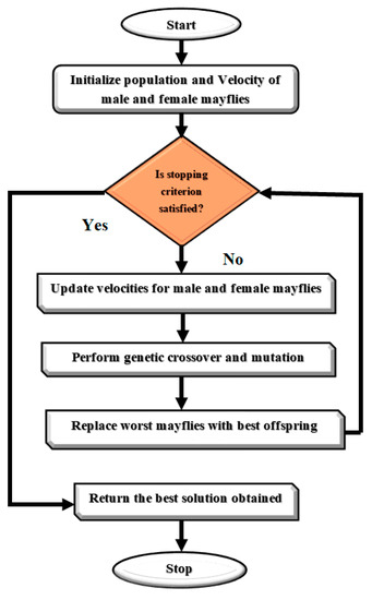
Figure 5.
Flowchart of MOA algorithm.
The MOA algorithm was modified and tailored for AD detection and classification by carefully defining the objective function, establishing the initial population of mayflies, updating and evaluating the algorithm, and comparing the results to other state-of-the-art methods. Algorithm 2 presents the modified MOA algorithm for AD Detection and Classification.
To define the objective function, we considered a set of features that are relevant for AD detection and classification, such as cortical thickness, hippocampal volume, and white matter hyper intensities. Based on these features, we then designed a fitness function that maximized the separation between healthy and diseased individuals. To establish the initial population of mayflies, we randomly generated a set of solutions for each feature in the objective function. We then assigned these solutions to a set of male and female mayflies with baseline velocities and evaluated their fitness using the objective function.
To update and evaluate the algorithm, we updated the velocities and solutions of the male and female mayflies, ranked the mayflies based on their fitness, mated the mayflies to generate offspring, evaluated the offspring’s fitness, separated the offspring randomly into male and female mayflies, and replaced the worst solutions with the best new ones. We also compared the results of our algorithm to other approaches, such as random forests and SVM, using metrics such as accuracy, sensitivity, and specificity.
By providing a more detailed explanation of how the Mayfly Optimization Algorithm was adapted for AD detection and classification, we can demonstrate the modifications and tailoring that were necessary to make the algorithm effective for this specific task. It can help readers understand the strengths and limitations of the algorithm and how it compares to other methods in the field.
| Algorithm 2 Mayfly Optimization Algorithm for AD detection and classification |
| Inputs: |
| - Dataset containing brain images (X) and corresponding labels (y) |
| - Population size (N) |
| - Maximum number of iterations (max_iter) |
| Outputs: |
| - Best set of features found (best_features) |
|
Equations:
- ➢
- Equation (1): male_velocity = rand() * male_velocity + rand() * (gbest − position)
- ➢
- Equation (2): female_velocity = rand() * female_velocity + rand() * (pbest − position)
- ➢
- Equation (3): male_position = male_position + male_velocity
- ➢
- Equation (4): female_position = female_position + female_velocity
- ➢
- Equation (5): offspring_position = rand() * (female1_position − female2_position) + female2_position
- ➢
- Equation (6): offspring_velocity = rand() * (female1_velocity − female2_velocity) + female2_velocity
- ➢
- Equation (7): new_feature_set = select_features(male_position)
The proposed Mayfly Optimization Algorithm for AD Detection and Classification is designed to identify the best set of features from brain MRI images that can be used to accurately classify patients with Alzheimer’s disease. The algorithm begins by pre-processing the MRI images and randomly selecting a subset of features to use for classification. It then initializes a population of female mayflies with random positions and velocities for the selected subset of features, as well as a population of male mayflies with random velocities for the same subset of features.
The algorithm then evaluates the classification performance of each female mayfly using a classifier and cross-validation on the selected subset of features, and sets the global best solution (gbest) to be the female mayfly with the highest classification performance. In the following iterations, the algorithm updates the subset of features used for classification by selecting features based on the positions of the male mayflies. It then evaluates the classification performance of each female mayfly using the updated subset of features and the classifier and updates the positions and velocities of male and female mayflies based on the updated subset of features.
Finally, the mayflies are ranked based on their classification performance, and the best new solutions are used to replace the worst solutions. The algorithm stops when the maximum number of iterations is reached or when a predetermined accuracy threshold is met. The proposed algorithm also includes visualizations of feature importance and/or saliency maps to help understand which parts of the brain are most important for classification and classification performance metrics such as accuracy and F1-score.
4. Result and Discussion
We have evaluated an existing model’s potential to foretell the development of AD over a period of 2.5 years. The ADNI database was combed through in order to get information on people who had participated in the ADNI. Practitioners can use the confusion matrix to help them gauge the results’ performance [12]. Patients who were correctly diagnosed as suffering from Alzheimer (TPs) and those who were not (TNs) were divided into three groups: those with AD (FNs), those without AD (FPs), and those who were misdiagnosed as TNs (FPs). False negative predictions are particularly dangerous in the medical field. The various metrics of performance were calculated using a confusion matrix. Accuracy was calculated based on the number of correctly identified events (Acc).
The square root of the Root Mean Squared Error (RMSE) reflects the average discrepancy between observed data and forecasted values. The equation used to calculate its worth is (19).
4.1. Precision
Tabulated results of a precision comparison of the DBN-MOA method to those of other existing methods are shown in Figure 6. The graph demonstrates how the ML approach led to improved precision and performance. By way of comparison, the SVM model, the RF model, the KNN model, the LR model, and the DT model all achieved precisions of 65.821%, 69.832%, 72.465%, 77.682%, and 83.312% with data set 100, respectively. However, DBN-MOA has demonstrated its best performance with varying sizes of data. Furthermore, under 600 data points, the precision values for the SVM, RF, KNN, LR, and DT models are 68.132%, 71.132%, 76.685%, 82.705%, and 88.932%, respectively, while the DBN-MOA model has a precision value of 94.621%.
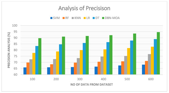
Figure 6.
Precision Analysis of the DBN-MOA method with the existing system.
4.2. Recall
Figure 7 illustrates a comparative recall examination of the DBN-MOA approach with other existing methods. With data set to 100, the recall value is 90.162% for DBN-MOA, whereas the SVM, RF, KNN, LR, and DT models have obtained recalls of 70.632%, 74.659%, 77.465%, 81.112%, and 85.652%, respectively.
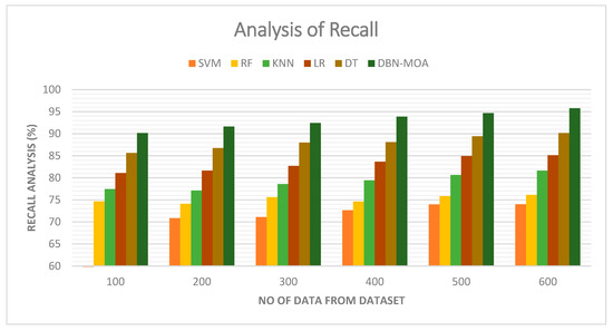
Figure 7.
Recall Analysis of the DBN-MOA method with the existing system.
However, the DBN-MOA model has shown maximum performance with different data sizes. Similarly, under 600 data points, the recall value of DBN-MOA is 95.789%, while it is 73.998%, 76.132%, 81.656%, 85.132%, and 90.162% for SVM, RF, KNN, LR, and DT models, respectively.
4.3. RMSE
Figure 8 shows the results of an RMSE comparison of the DBN-MOA method to those of other existing methods. The lower RMSE value achieved by the ML method is graphically displayed in the figure. On data set 100, for instance, the RMSE is 20.685%, while the SVM, RF, KNN, LR, and DT models achieve marginally improved RMSE of 45.839%, 36.811%, 32.851%, 28.652, and 24.685%, respectively. In contrast, the DBN-MOA model has demonstrated its best performance across various data sizes while maintaining a small RMSE. Similarly, under 600 data points, the RMSE values for SVM, RF, KNN, LR, and DT models are 52.965%, 44.832%, 36.789%, 31.789, and 27.981%, respectively, while DBN-RMSE MOA’s value is 23.785%.
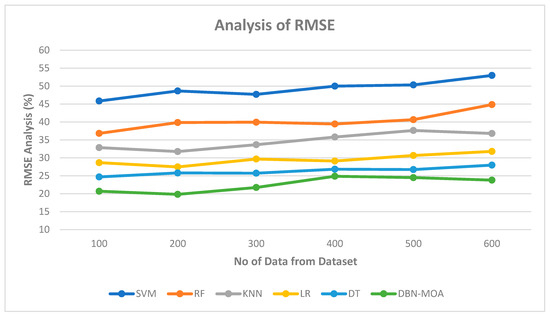
Figure 8.
RMSE Analysis of the DBN-MOA method with the existing system.
4.4. F-Score
Figure 9 shows the results of an f-score analysis comparing the DBN-MOA approach to those of other existing methods. The improved performance measured by an f-score is evidenced graphically to have resulted from the ML method. For instance, on data set 100, the f-score for DBN-MOA is 88.132%, while those for SVM, RF, KNN, LR, and DT are 60.832%, 64.981%, 69.382%, 75.659%, and 82.132%. However, DBN-MOA has demonstrated its best performance with varying sizes of data. Similarly, under 600 data points, the f-score values for SVM, RF, KNN, LR, and DT models are 63.805%, 68.465%, 74.168%, 80.435%, and 87.652%, respectively, while the f-score value for DBN-MOA is 93.187%.
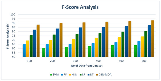
Figure 9.
F-Score Analysis of the DBN-MOA method with the existing system.
4.5. Execution Time
Figure 10 describes the execution time analysis of the DBN-MOA technique with existing methods. The data clearly shows that the DBN-MOA method has outperformed the other techniques in all aspects. For example, with 100 pieces of data, the DBN-MOA method has taken only 1.384 s to execute, while the other existing techniques like SVM, RF, KNN, LR, and DT have an execution time of 7.762 s, 6.465 s, 5.484 s, 3.732 s, and 2.981 s, respectively. Similarly, for 600 data points, the DBN-MOA method has an execution time of 2.4 s while the other existing techniques like SVM, RF, KNN, LR, and DT have 8.990 s, 6.965 s, 5.693 s, 4.382 s, and 2.999 s of execution time, respectively.
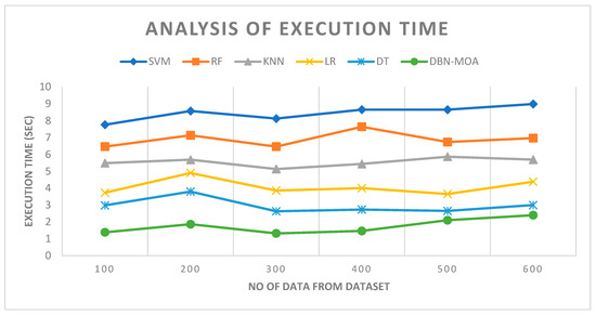
Figure 10.
Execution Time Analysis of the DBN-MOA method with the existing system.
4.6. Accuracy
Accuracy comparisons of the DBN-MOA method to those of other existing methods are shown in Figure 11. Improved performance and accuracy can be seen in the graph, demonstrating the success of the ML method.
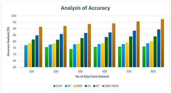
Figure 11.
Accuracy Analysis of the DBN-MOA method with the existing system.
To illustrate, the accuracy of DBN-MOA is 91.435% on data set 100, while the corresponding values for SVM, RF, KNN, LR, and DT models are 74.982%, 77.182%, 78.732%, 81.565%, and 84.78%, respectively. However, DBN-MOA has demonstrated its best performance with varying sizes of data. Comparatively, under 600 data points, the accuracy values for the SVM, RF, KNN, LR, and DT models are 76.112%, 78.685%, 80.166%, 83.966%, and 89.465%, respectively, while the DBN-MOA model has a value of 97.456%.
5. Conclusions
This research examines the strengths and weaknesses of various MRI-based AD detection strategies. Several reliable approaches to AD classification have been proposed and implemented. Research that combines ML and neuroscience can lead to a more accurate diagnosis of AD. In this article, we tested a model for predicting the onset of AD using the ADNI dataset. The ADNI database currently contains information on 1029 people who met the inclusion criteria. It was proposed to use supervised learning classifiers in the form of a DBN to identify AD in dementia patients by analyzing features from a longitudinal brain MRI scan of patients using IoT based portable MRI scan machine to obtain real-time imaging. Incorporating a richer set of cost-effective time-series features, such as patients’ comorbidities, cognitive scores, medication histories, and demographics, led to the superior performance of our DBN-MOA models compared to state-of-the-art methods. Our results demonstrate the universal benefit of early feature fusion, and they particularly highlight the value of fusing diagnostic and therapeutic features. When comparing accuracy, the random forest model is superior. SVM, RF, KNN, LR, and DT were tested, and their results were compared. The proposed DBN-MOA method can distinguish between healthy and ill patients with an accuracy of 97.456%, r-Score of 93.187%, recall of 95.789% and precision of 94.621% achieved by the proposed technique. The results demonstrate that the proposed DBN-MOA model clearly outclasses the existing models and performs better on all the parameters of accuracy, f-Score, recall and precision. The results validate that the proposed model is efficient and better than the existing models. The future of assessing the efficacy of multiclass AD stage classifications will involve using Efficient Net B0-B7 and other pre-trained models. The dataset is also enlarged through the use of elementary data augmentation techniques. Further, Alzheimer’s characteristics will be highlighted via MRI segmentation before AD stage classifications are made.
Author Contributions
Conceptualization, N.A., S.A., S.B.K. and I.A.; formal analysis, M.S., I.M.K. and A.A.M.; investigation, S.B.K., I.A., N.A., S.A. and M.S.; project administration, N.A., S.B.K. and A.A.M.; resources, A.A.M.; supervision, S.B.K. and A.A.M.; visualization, M.S. and I.M.K.; writing—original draft, M.S., N.A., S.A. and S.B.K.; writing—review and editing, I.A., I.M.K. and A.A.M. All authors have read and agreed to the published version of the manuscript.
Funding
This research is supported by Princess Nourah bint Abdulrahman University, Researchers Supporting Project Number (PNURSP2023R151), Princess Nourah bint Abdulrahman University, Riyadh, Saudi Arabia.
Institutional Review Board Statement
Not applicable.
Informed Consent Statement
Not applicable.
Data Availability Statement
Publicly available datasets were analyzed in this study. This data can be found here: https://adni.loni.usc.edu/data-samples/adni-data-inventory/ (accessed on 11 January 2023).
Conflicts of Interest
The author declares no conflict of interest.
References
- Ahmad, F.B.; Anderson, R.N. The Leading Causes of Death in the US for 2020. JAMA 2021, 325, 1829–1830. [Google Scholar] [CrossRef]
- Das, R.; Rauf, A.; Akhter, S.; Islam, M.N.; Emran, T.B.; Mitra, S.; Khan, I.N.; Mubarak, M.S. Role of Withaferin A and Its Derivatives in the Management of Alzheimer’s Disease: Recent Trends and Future Perspectives. Molecules 2021, 26, 3696. [Google Scholar] [CrossRef]
- Turner, R.S.; Stubbs, T.; Davies, D.A.; Albensi, B.C. Potential New Approaches for Diagnosis of Alzheimer’s Disease and Related Dementias. Front. Neurol. 2020, 11, 496. [Google Scholar] [CrossRef]
- Wu, C.-L.; Lin, T.-J.; Chiou, G.-L.; Lee, C.-Y.; Luan, H.; Tsai, M.-J.; Potvin, P.; Tsai, C.-C. A Systematic Review of MRI Neuroimaging for Education Research. Front. Psychol. 2021, 12, 617599. [Google Scholar] [CrossRef]
- Alam, S.; Shuaib, M.; Ahmad, S.; Jayakody, D.N.K.; Muthanna, A.; Bharany, S.; Elgendy, I.A. Blockchain-Based Solutions Supporting Reliable Healthcare for Fog Computing and Internet of Medical Things (IoMT) Integration. Sustainability 2022, 14, 15312. [Google Scholar] [CrossRef]
- Gaubert, S.; Houot, M.; Raimondo, F.; Ansart, M.; Corsi, M.-C.; Naccache, L.; Sitt, J.D.; Habert, M.-O.; Dubois, B.; Fallani, F.D.V. A Machine Learning Approach to Screen for Preclinical Alzheimer’s Disease. Neurobiol. Aging 2021, 105, 205–216. [Google Scholar] [CrossRef]
- Gao, Z.; Pan, X.; Shao, J.; Jiang, X.; Su, Z.; Jin, K.; Ye, J. Automatic interpretation and clinical evaluation for fundus fluorescein angiography images of diabetic retinopathy patients by deep learning. Br. J. Ophthalmol. 2022, 321472. [Google Scholar] [CrossRef]
- Battineni, G.; Sagaro, G.G.; Chinatalapudi, N.; Amenta, F. Applications of Machine Learning Predictive Models in the Chronic Disease Diagnosis. J. Pers. Med. 2020, 10, 21. [Google Scholar] [CrossRef]
- Spooner, A.; Chen, E.; Sowmya, A.; Sachdev, P.; Kochan, N.A.; Trollor, J.; Brodaty, H. A Comparison of Machine Learning Methods for Survival Analysis of High-Dimensional Clinical Data for Dementia Prediction. Sci. Rep. 2020, 10, 20410. [Google Scholar] [CrossRef]
- Nori, V.S.; Hane, C.A.; Crown, W.H.; Au, R.; Burke, W.J.; Sanghavi, D.M.; Bleicher, P. Machine Learning Models to Predict Onset of Dementia: A Label Learning Approach. Alzheimer’s Dement. Transl. Res. Clin. Interv. 2019, 5, 918–925. [Google Scholar] [CrossRef]
- Saab, S., Jr.; Saab, K.; Phoha, S.; Zhu, M.; Ray, A. A multivariate adaptive gradient algorithm with reduced tuning efforts. Neural Netw. 2022, 152, 499–509. [Google Scholar] [CrossRef] [PubMed]
- Saab, S., Jr.; Fu, Y.; Ray, A.; Hauser, M. A dynamically stabilized recurrent neural network. Neural Process. Lett. 2022, 54, 1195–1209. [Google Scholar] [CrossRef]
- Jo, T.; Nho, K.; Saykin, A.J. Deep Learning in Alzheimer’s Disease: Diagnostic Classification and Prognostic Prediction Using Neuroimaging Data. Front. Aging Neurosci. 2019, 11, 220. [Google Scholar] [CrossRef] [PubMed]
- Bashir, M.F.; Javed, A.R.; Arshad, M.U.; Gadekallu, T.R.; Shahzad, W.; Beg, M.O. Context aware emotion detection from low resource urdu language using deep neural network. Trans. Asian Low-Resour. Lang. Inf. Process. 2023, 22, 1–30. [Google Scholar] [CrossRef]
- Lundervold, A.S.; Lundervold, A. An Overview of Deep Learning in Medical Imaging Focusing on MRI. Z. Med. Phys. 2019, 29, 102–127. [Google Scholar] [CrossRef]
- Battineni, G.; Chintalapudi, N.; Amenta, F. Comparative Machine Learning Approach in Dementia Patient Classification Using Principal Component Analysis. Group 2020, 500, 146. [Google Scholar]
- Aditya, C.R.; Pande, M.B.S. Devising an Interpretable Calibrated Scale to Quantitatively Assess the Dementia Stage of Subjects with Alzheimer’s Disease: A Machine Learning Approach. Inform. Med. Unlocked 2017, 6, 28–35. [Google Scholar] [CrossRef]
- Lian, Z.; Zeng, Q.; Wang, W.; Gadekallu, T.R.; Su, C. Blockchain-Based Two-Stage Federated Learning with Non-IID Data in IoMT System. IEEE Trans. Comput. Soc. Syst. 2022. [Google Scholar] [CrossRef]
- Judith, A.M.; Priya, S.B.; Mahendran, R.K.; Gadekallu, T.R.; Ambati, L.S. Two-phase classification: ANN and A-SVM classifiers on motor imagery BCI. Asian J. Control 2022. [Google Scholar] [CrossRef]
- Alam, S.; Bhatia, S.; Shuaib, M.; Khubrani, M.M.; Alfayez, F.; Malibari, A.A.; Ahmad, S. An Overview of Blockchain and IoT Integration for Secure and Reliable Health Records Monitoring. Sustainability 2023, 15, 5660. [Google Scholar] [CrossRef]
- Siyu Lu, J.Y.B.Y. Analysis and Design of Surgical Instrument Localization Algorithm. Comput. Model. Eng. Sci. 2023, 137, 669–685. [Google Scholar]
- Singh, A.; Joshi, K.; Alam, S.; Bharany, S.; Shuaib, M.; Ahmad, S. Internet of Things-Based Integrated Remote Electronic Health Surveillance and Alert System: A Review. In Proceedings of the 2022 IEEE International Conference on Current Development in Engineering and Technology (CCET), Bhopal, India, 23–24 December 2022; IEEE: Piscataway, NJ, USA, 2022; pp. 1–6. [Google Scholar]
- Cao, P.; Liu, X.; Yang, J.; Zhao, D.; Huang, M.; Zaiane, O. ℓ2,1 − ℓ1 Regularized Nonlinear Multi-Task Representation Learning Based Cognitive Performance Prediction of Alzheimer’s Disease. Pattern Recognit. 2018, 79, 195–215. [Google Scholar] [CrossRef]
- Nawaz, H.; Maqsood, M.; Afzal, S.; Aadil, F.; Mehmood, I.; Rho, S. A Deep Feature-Based Real-Time System for Alzheimer Disease Stage Detection. Multimed. Tools Appl. 2021, 80, 35789–35807. [Google Scholar] [CrossRef]
- Feng, C.; Elazab, A.; Yang, P.; Wang, T.; Lei, B.; Xiao, X. 3D Convolutional Neural Network and Stacked Bidirectional Recurrent Neural Network for Alzheimer’s Disease Diagnosis. In Proceedings of the PRedictive Intelligence in MEdicine: First International Workshop, PRIME 2018, Held in Conjunction with MICCAI 2018, Granada, Spain, 16 September 2018; Proceedings 1; Springer: Berlin/Heidelberg, Germany, 2018; pp. 138–146. [Google Scholar]
- Venugopalan, J.; Tong, L.; Hassanzadeh, H.R.; Wang, M.D. Multimodal Deep Learning Models for Early Detection of Alzheimer’s Disease Stage. Sci. Rep. 2021, 11, 3254. [Google Scholar] [CrossRef]
- AI-Atroshi, C.; Rene Beulah, J.; Singamaneni, K.K.; Pretty Diana Cyril, C.; Neelakandan, S.; Velmurugan, S. Automated Speech Based Evaluation of Mild Cognitive Impairment and Alzheimer’s Disease Detection Using with Deep Belief Network Model. Int. J. Healthc. Manag. 2022, 1–11. [Google Scholar] [CrossRef]
- Ramzan, F.; Khan, M.U.G.; Rehmat, A.; Iqbal, S.; Saba, T.; Rehman, A.; Mehmood, Z. A Deep Learning Approach for Automated Diagnosis and Multi-Class Classification of Alzheimer’s Disease Stages Using Resting-State FMRI and Residual Neural Networks. J. Med. Syst. 2020, 44, 37. [Google Scholar] [CrossRef]
- Mehmood, A.; Maqsood, M.; Bashir, M.; Shuyuan, Y. A Deep Siamese Convolution Neural Network for Multi-Class Classification of Alzheimer Disease. Brain Sci. 2020, 10, 84. [Google Scholar] [CrossRef]
- Jain, R.; Jain, N.; Aggarwal, A.; Hemanth, D.J. Convolutional Neural Network Based Alzheimer’s Disease Classification from Magnetic Resonance Brain Images. Cogn. Syst. Res. 2019, 57, 147–159. [Google Scholar] [CrossRef]
- Sarraf, S.; Tofighi, G. Classification of Alzheimer’s Disease Using Fmri Data and Deep Learning Convolutional Neural Networks. arXiv 2016, arXiv:1603.08631. [Google Scholar]
- Afzal, S.; Maqsood, M.; Nazir, F.; Khan, U.; Aadil, F.; Awan, K.M.; Mehmood, I.; Song, O.-Y. A Data Augmentation-Based Framework to Handle Class Imbalance Problem for Alzheimer’s Stage Detection. IEEE Access 2019, 7, 115528–115539. [Google Scholar] [CrossRef]
- Aderghal, K.; Khvostikov, A.; Krylov, A.; Benois-Pineau, J.; Afdel, K.; Catheline, G. Classification of Alzheimer Disease on Imaging Modalities with Deep CNNs Using Cross-Modal Transfer Learning. In Proceedings of the 2018 IEEE 31st international symposium on computer-based medical systems (CBMS), Karlstad, Sweden, 18–21 June 2018; IEEE: Piscataway, NJ, USA, 2018; pp. 345–350. [Google Scholar]
- Spasov, S.; Passamonti, L.; Duggento, A.; Lio, P.; Toschi, N.; Initiative, A.D.N. A Parameter-Efficient Deep Learning Approach to Predict Conversion from Mild Cognitive Impairment to Alzheimer’s Disease. Neuroimage 2019, 189, 276–287. [Google Scholar] [CrossRef]
- Wang, H.; Shen, Y.; Wang, S.; Xiao, T.; Deng, L.; Wang, X.; Zhao, X. Ensemble of 3D Densely Connected Convolutional Network for Diagnosis of Mild Cognitive Impairment and Alzheimer’s Disease. Neurocomputing 2019, 333, 145–156. [Google Scholar] [CrossRef]
- Huang, L.; Jin, Y.; Gao, Y.; Thung, K.-H.; Shen, D.; Initiative, A.D.N. Longitudinal Clinical Score Prediction in Alzheimer’s Disease with Soft-Split Sparse Regression Based Random Forest. Neurobiol. Aging 2016, 46, 180–191. [Google Scholar] [CrossRef]
- Kundaram, S.S.; Pathak, K.C. Deep Learning-Based Alzheimer Disease Detection. In Proceedings of the Fourth International Conference on Microelectronics, Computing and Communication Systems: MCCS 2019, Ranchi, India, 11–12 May 2019; Springer: Berlin/Heidelberg, Germany, 2021; pp. 587–597. [Google Scholar]
- Vyas, A.H.; Mehta, M.A.; Kotecha, K.; Pandya, S.; Alazab, M.; Gadekallu, T.R. Tear Film Breakup Time-Based Dry Eye Disease Detection Using Convolutional Neural Network. Neural Comput. Appl. 2022, 1–19. [Google Scholar] [CrossRef]
- Bhatia, S.; Alam, S.; Shuaib, M.; Alhameed, M.H.; Jeribi, F.; Alsuwailem, R.I. Retinal Vessel Extraction via Assisted Multi-Channel Feature Map and U-Net. Front. Public Health 2022, 10, 858327. [Google Scholar] [CrossRef]
- Mishra, R.K.; Urolagin, S.; Jothi, J.A.A.; Neogi, A.S.; Nawaz, N. Deep Learning-Based Sentiment Analysis and Topic Modeling on Tourism during Covid-19 Pandemic. Front. Comput. Sci. 2021, 3, 775368. [Google Scholar] [CrossRef]
- Tripathy, B.K.; Parimala, M.; Reddy, G.T. Innovative Classification, Regression Model for Predicting Various Diseases. In Data Analytics in Biomedical Engineering and Healthcare; Elsevier: Amsterdam, The Netherlands, 2021; pp. 179–203. [Google Scholar]
- Zhang, Y.; Wang, S.; Sui, Y.; Yang, M.; Liu, B.; Cheng, H.; Sun, J.; Jia, W.; Phillips, P.; Gorriz, J.M. Multivariate Approach for Alzheimer’s Disease Detection Using Stationary Wavelet Entropy and Predator-Prey Particle Swarm Optimization. J. Alzheimer’s Dis. 2018, 65, 855–869. [Google Scholar] [CrossRef]
- Korolev, S.; Safiullin, A.; Belyaev, M.; Dodonova, Y. Residual and Plain Convolutional Neural Networks for 3D Brain MRI Classification. In Proceedings of the 2017 IEEE 14th international symposium on biomedical imaging (ISBI 2017), Melbourne, Australia, 18–21 April 2017; IEEE: Piscataway, NJ, USA, 2017; pp. 835–838. [Google Scholar]
- Ding, Y.; Sohn, J.H.; Kawczynski, M.G.; Trivedi, H.; Harnish, R.; Jenkins, N.W.; Lituiev, D.; Copeland, T.P.; Aboian, M.S.; Mari Aparici, C. A Deep Learning Model to Predict a Diagnosis of Alzheimer Disease by Using 18F-FDG PET of the Brain. Radiology 2019, 290, 456–464. [Google Scholar] [CrossRef]
- Beheshti, I.; Demirel, H.; Farokhian, F.; Yang, C.; Matsuda, H.; Initiative, A.D.N. Structural MRI-Based Detection of Alzheimer’s Disease Using Feature Ranking and Classification Error. Comput. Methods Programs Biomed. 2016, 137, 177–193. [Google Scholar] [CrossRef]
- Alzheimer’s Disease Neuroimaging Initiative (ADNI). Availabel online: https://adni.loni.usc.edu/ (accessed on 11 January 2023).
- Naz, S.; Ashraf, A.; Zaib, A. Transfer Learning Using Freeze Features for Alzheimer Neurological Disorder Detection Using ADNI Dataset. Multimed. Syst. 2022, 28, 85–94. [Google Scholar] [CrossRef]
- Zervoudakis, K.; Tsafarakis, S. A Mayfly Optimization Algorithm. Comput. Ind. Eng. 2020, 145, 106559. [Google Scholar] [CrossRef]


Disclaimer/Publisher’s Note: The statements, opinions and data contained in all publications are solely those of the individual author(s) and contributor(s) and not of MDPI and/or the editor(s). MDPI and/or the editor(s) disclaim responsibility for any injury to people or property resulting from any ideas, methods, instructions or products referred to in the content. |
© 2023 by the authors. Licensee MDPI, Basel, Switzerland. This article is an open access article distributed under the terms and conditions of the Creative Commons Attribution (CC BY) license (https://creativecommons.org/licenses/by/4.0/).