Multi-Objective Collaborative Control Method for Multi-Axle Distributed Vehicle Assisted Driving

Abstract

For human–machine collaborative driving conditions, a hierarchical chassis multi-objective cooperative control method is proposed in this paper. Firstly, based on the phase plane theory, vehicle dynamics analysis is carried out to complete the definition of vehicle stability region. Secondly, based on the linear time-varying (LTV) system model, a cooperative control strategy combining fuzzy control with model predictive control (MPC) is proposed in the upper layer. In this strategy, the assisted driving weight adjustment coefficient and the stability weight adjustment coefficient are obtained by fuzzy mapping combining human–machine cooperation index and the vehicle stability region, respectively, and the optimization objectives of MPC are designed based on the above coefficients. In the lower layer torque allocation strategy, the stability weight adjustment coefficient is introduced to achieve multi-objective optimization of tire load rate and energy efficiency. For energy efficiency optimization, an optimal energy efficiency point-based tracking method is proposed to avoid nonlinearity caused by the introduction of motor loss models. Simulation analysis results show that the proposed strategy can effectively alleviate human–machine conflicts and improve vehicle handing stability. It also can achieve smaller tire load rate optimization through torque allocation and can reduce energy consumption by approximately 8% compared with the inter-axle torque allocation strategy. This study helps to promote the improvement of the comprehensive performance of assisted driving vehicles in human–machine cooperation, handling stability, and energy-saving torque distribution.

1. Introduction

Electrification and intelligence are the two major directions for the future development of automobiles [1]. Electric transmission technology not only solves energy and pollution problems but also has more advantages than conventional vehicles. For example, distributed electric drive technology is a new configuration of electric transmission technology, eliminating the need for transmissions and differentials in traditional drive systems, saving chassis space, and improving transmission efficiency. And distributed drive technology enables independent and precise control of the torque of each wheel drive, which helps achieve multi-objective coupling control of vehicle handling, safety, and other aspects [2,3]. The intelligence level of multi-axle heavy vehicles is relatively low, and their larger body size and higher cockpit increase the difficulty of driver control and also increase driving risks. Assisted driving technology, as an important part of intelligent driving technology, is a compromise solution that involves the driver and the machine completing driving tasks together [4,5]. It helps to improve the driving safety of multi-axle heavy vehicles before achieving fully automated driving.

Assisted driving can be divided into two forms: indirect assisted driving and direct assisted driving [6,7]. Direct assisted driving is where the control applied by the driver and the assisted system is coupled and applied to the actuator, such as the electric power steering system (EPS). In this mode, the driver can simultaneously perceive the auxiliary torque applied by the system. In contrast to indirect assisted driving, the driver has ultimate control of the vehicle, while the continuous tactile feedback helps maintain the driver’s level of presence in the loop and enhances the driver’s trust in the system. Of course, inconsistent human–machine intentions in the assisted driving process can lead to control conflicts, and this has been the subject of much research. The authors of [8] first established a driver’s two-point preview model, which is combined with the U-shaped function method to characterize the driver’s assistance needs. Then, the Takagi–Sugeno multi-model method was used to achieve assisted lane maintenance and obstacle avoidance for the driver. The authors of [9] defined the driver’s activity and human–machine cooperation index and used fuzzy logic to adjust assistance weights in real time. It finally used LMI optimization to design an adaptive shared controller, ensuring closed-loop stability while greatly reducing human–machine conflicts during coupled driving processes. Professor Na’s team has conducted a lot of research on direct assisted driving strategies related to game theory. They first used game theory to analyze human–machine driving rights interactions and established four interaction paradigms: distributed, non-cooperative Nash, non-cooperative Stackelberg, and cooperative Pareto [10].

Many scholars have researched multi-objective optimal control of distributed vehicle dynamics, aiming to improve the safety, stability, handling, and energy economy of the vehicle. Hierarchical control structures are currently the most widely used due to their flexibility in control design, clear division of labor, and efficient operation. Hierarchical control is generally divided into upper and lower layers, where the upper layer tracks or optimizes target variables related to vehicle dynamics, and the lower layer distributes torque. The core of the upper layer controller is direct yaw moment control (DYC), as well as the control forms derived from DYC, such as active front wheel steering (AFS) combined with DYC, active rear wheel steering (RWS) combined with DYC, etc. A robust sliding mode predictive control (SMPC) strategy was proposed to solve a multi-objective multi-constraint optimization problem, which first determined the current vehicle stability based on a phase plane analysis method and combined the driver’s future driving state prediction with a fuzzy control algorithm to obtain weight coefficients to coordinate AFS and DYC [11]. Guo et al. [12,13] proposed a real-time nonlinear model predictive control (NMPC) strategy to solve the direct yaw moment control problem, and for the first time, an extended/generalized minimum residual (C/GMRES) algorithm was used for nonlinear optimization and real-time solution. A real-time nonlinear model predictive control strategy combining DYC and RWS was proposed in the literature [14], using Pontryagin’s principle of minimum (PMP)-based algorithm for fast solution of nonlinear optimization problems, which has better handling stability compared to the pure DYC method. For the lower-layer torque allocation problem, the literature [15] realized the reconfiguration distribution of the lower layer motor torque by adjusting the quadratic form distribution matrix and used the sliding mode control (SMC) algorithm to calculate the modified torque to keep each tire within the optimal slip ratio. Adeleke et al. [16] proposed a dynamic programming algorithm (DP) to solve the economical problem of torque distribution.

Current research on human–machine co-driving has focused only on the allocation of human–machine driving privileges, ignoring the optimal control of vehicle dynamics. For the multi-axle heavy vehicle studied in this paper, due to the large inertia of the vehicle itself, if only the front wheel steering is used for assisted driving motion control, its handling will inevitably be poor. At the same time, when the tires enter the nonlinear region, the vehicle is also more prone to instability. Therefore, it is necessary to comprehensively consider the allocation of human–machine driving permissions and the collaborative optimization of the handling and stability performance of multi-axle vehicles in the control of assisted driving. The chassis control performance of human–machine collaborative driving conditions is also inseparable from the reasonable allocation of torque for distributed electric drive vehicles. In the study of lower-layer torque allocation, efficient torque distribution with multiple objectives such as energy saving and tire loading is still one of the difficulties in research due to the nonlinearity of the energy consumption relationship of the drive system and the redundancy of the execution components of distributed multi-axle vehicles.

Therefore, a multi-objective collaborative control method for multi-axle distributed vehicle assisted driving chassis is proposed in this article, and the overall control framework is shown in Figure 1. The control method includes the fuzzy cooperative control strategy based on LTV-MPC at the upper layer and the torque distribution strategy at the lower layer. In the upper-layer controller, the LTV system control model is established first, which combines the steering model, the two-degree-of-freedom (2DOF), model and the path tracking model. Secondly, using the phase plane analysis method, the critical conditions of vehicle stability and the linear operation of vehicle tires are analyzed. Finally, the critical stable steering angle ${\delta }_{1c}$ and linear critical steering angle ${\delta }_{1l}$ of the vehicle under different conditions are calibrated, and the state region of the vehicle is defined. In the fuzzy cooperative control strategy, the human–machine cooperation index $CI$ is defined, and the assisted driving weight adjustment coefficient ${\lambda }_r$ is obtained by fuzzy rule mapping. The stability weight adjustment coefficient ${\lambda }_{\beta }$ is obtained by mapping the steering angle and the rate of the steering angle, where the membership function of the steering angle is designed based on the obtained vehicle state region. Finally, the cost function of LTV-MPC is designed with the weight adjustment coefficient, the optimal auxiliary torque and generalized additional yaw moment are obtained, and the coordination between man–machine and vehicle handing stability in the auxiliary driving process is realized. Lower layer torque allocation, while meeting the requirements of tracking the target generalized longitudinal force and additional yaw moment, introduces the stability weight adjustment coefficient to achieve multi-objective optimization of tire load rate and energy efficiency. Then, an optimal energy efficiency point-based tracking method is proposed to achieve the optimization of multi-axle vehicle efficiency, avoiding the nonlinearity caused by considering energy consumption models and efficiently achieving torque distribution.

This study effectively improves the integrated control performance of distributed multi-axle vehicle chassis under man–machine cooperative driving conditions. The main contributions are as follows:

(1)

The stability region of the vehicle is obtained by the phase plane method. Based on this, the stability weight adjustment coefficient is obtained by fuzzy control mapping. At the same time, the LTV-MPC optimization problem is designed by combining the auxiliary driving and stability weight adjustment coefficient, then the multi-objective cooperation between man–machine co-driving and vehicle handling stability is realized.

(2)

Coordinate the multi-objective optimization between tire load rate and energy efficiency in torque distribution through the stability weight adjustment coefficient. The optimal energy efficiency point tracking strategy is adopted to achieve energy efficiency optimization, avoid nonlinear optimization solutions, and improve torque distribution efficiency.

2. Fuzzy Cooperative Control Strategy Based on LTV-MPC

2.1. Assisted Driving Control Model

The controlled object is a five-axle heavy vehicle with an assisted steering system, which acts on the first two axles. The assisted steering system is a coupled assisted steering system, which works by outputting assisted steering torque through the assisted steering motor, coupling with the driver’s input torque and the steering system’s aligning torque, and ultimately forming a steering angle response to assist in controlling the vehicle. Meanwhile, each wheel can be controlled independently and precisely by torque. This section builds a path tracking model for assisted driving, including a steering system model, the 2-DOF vehicle model, and the path-tracking model.

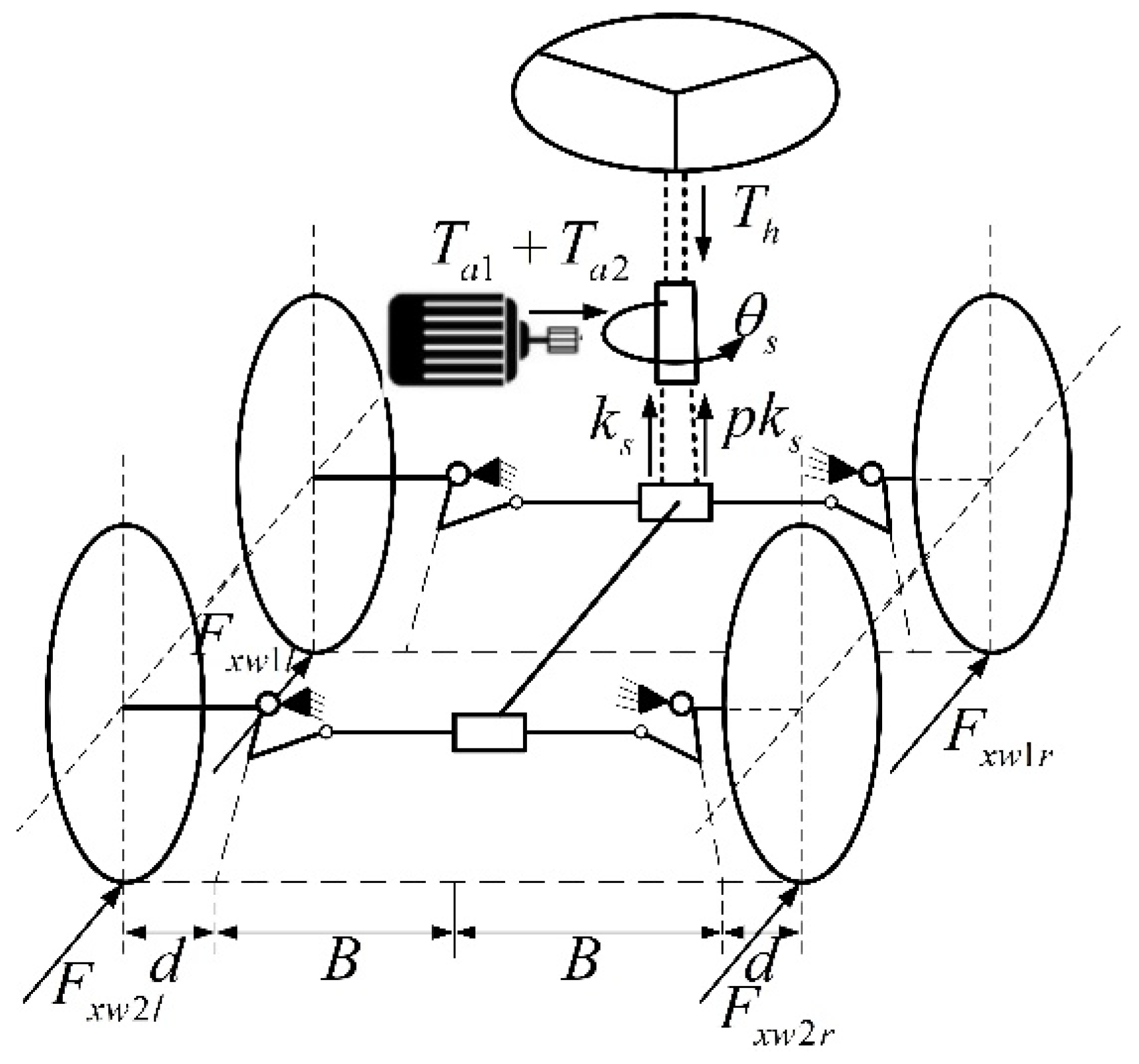
The structure of the assisted steering system model is shown in Figure 2. The assisted steering system includes the first and second axles, with the steering column between the steering wheel and the axle, and the steering dynamics are analyzed with the steering column as the object. The transmission between the steering column and the axle is carried out through gear and rack, and the transmission ratios between the gear and rack and the first and second axles are $k_s$ and $p\cdot k_s$, respectively. Here, $k_s>1,p=1.25$. The active force received by the assisted steering system includes the torque $T_h$ applied by the driver through the steering wheel and the assisted steering motor’s assisted torque $T_a$, which includes the driver assistance component $T_{a1}$ and the auxiliary component $T_{a2}$. $T_{a1}$ and $T_{a2}$ all act directly on the steering column. $T_{a1}$ achieves fixed proportion torque assistance for the driver, meeting $T_{a1}=k_h{T}_h$. Meanwhile, the system is also subjected to differential torque $M_{di}$ and aligning torque $M_{si}$ acting on the tires of the first and second axles, where differential torque is generated due to inconsistent longitudinal force allocation between the left and right tires. The dynamic equation of the assisted steering system can be expressed as:

$$\begin{array}{c}{J}_s{\ddot{\theta }}_s+b_s{\dot{\theta }}_s=T_h+T_{a1}+T_{a2}+\frac{M_{d1}}{k_s}+\frac{M_{d2}}{p\cdot k_s}-\frac{M_{s1}}{k_s}-\frac{M_{s2}}{p\cdot k_s}\end{array}$$

(1)

In the formula, $J_s$ is the equivalent moment of inertia of the steering column, $b_s$ is the equivalent damping, ${\theta }_s$ is the steering column angle. The aligning torque $M_{si}$ mainly consists of the lateral force $M_{syi}$ of the tire and the component of the aligning torque of the tire $M_{zzi}$, which can be expressed as:

$$\begin{array}{c}{M}_{si}=M_{syi}+M_{zzi}\approx F_{yi}\cdot R_w\cdot \tau +M_{zi}\end{array}$$

(2)

where $F_{yi}$ and $M_{zi}$ are the total lateral force and total aligning torque of the corresponding axle, $R_w$ is the wheel radius, and $\tau$ is the caster angle.

Due to the fact that differential torque $M_{di}$ is obtained from the lower layer torque allocation results, the output torque of the auxiliary steering motor serves as another controllable active force, which can balance the impact of differential torque when necessary to achieve precise control of the steering system. Therefore, the consideration of differential torque $M_{di}$ is temporarily ignored in the control model, and the actual output torque of the final auxiliary motor can be calculated by the driver assistance component $T_{a1}$, the auxiliary component $T_{a2}$, and the differential torque $M_{di}$. The steering system model can be represented as:

$$\begin{array}{c}{J}_s{\ddot{\theta }}_s+b_s{\dot{\theta }}_s=T_h+T_{a1}+T_{a2}-\frac{F_{y1}\cdot R_w\cdot \tau +M_{z1}}{k_s}-\frac{F_{y1}\cdot R_w\cdot \tau +M_{z1}}{p\cdot k_s}\end{array}$$

(3)

The 2-DOF vehicle dynamics model is chosen for the control model, and the force analysis of the 2-DOF vehicle dynamics model is shown in Figure 3.

The model considers the influence of generalized additional yaw moment $M_d$ on yaw motion, and the 2-DOF vehicle model is represented as follows:

$$\begin{array}{c}\left\{\begin{array}{c}m\left(v_x\dot{\beta }+v_x{\omega }_z\right)={\displaystyle {\displaystyle \sum }_{i=1}^5}{F}_{yi}\\ I_z{\dot{\omega }}_z={\displaystyle {\displaystyle \sum }_{i=1}^2}{L}_i{F}_{yi}-{\displaystyle {\displaystyle \sum }_{i=3}^5}{L}_i{F}_{yi}+M_d\end{array}\right.\end{array}$$

(4)

where $m$ is the total vehicle mass, $v_x$ is the longitudinal speed, $I_z$ is the yaw inertia of the entire vehicle. $L_i$ represents the distance from each axle to the center of gravity (CG). Vehicle sideslip angle and yaw rate can be expressed as $\beta$and ${\omega }_z$.

The path tracking model can be represented as

$$\begin{array}{c}\left\{\begin{array}{c}{\dot{y}}_e\approx v_x{\psi }_e+v_x\beta \\ {\dot{\psi }}_e={\omega }_z-v_x\rho \end{array}\right.\end{array}$$

(5)

where $y_e$ is the lateral distance error, ${\psi }_e$ is the heading angle error, and $\rho$ is the path curvature.

Organize (3)–(5) to obtain the control system model as shown below:

$$\dot{\mathit{x}}=f\left(\mathit{x},\mathit{u},\mathit{w}\right)=\left[\begin{array}{c}{\dot{\theta }}_s\\ \frac{\left(-b_s{\dot{\theta }}_s+T_h+T_{a1}+T_{a2}^n\right)}{J_s}-\frac{\left(F_{y1}{R}_w\tau +M_{z1}\right)}{\left(k_s{J}_s\right)}-\frac{\left(F_{y2}{R}_w\tau +M_{z2}\right)}{\left(p{k}_s{J}_s\right)}\\ \frac{{\sum }_{i=1}^5{F}_{yi}}{\left(m{v}_x\right)}-{\omega }_z\\ \frac{\left({\sum }_{i=1}^2\left(L_i{F}_{yi}\right)-{\sum }_{i=3}^5\left(L_i{F}_{yi}\right)\right)}{I_z}+\frac{M_d}{I_z}\\ v_x{\psi }_e+v_x\beta \\ {\omega }_z-v_x\rho \end{array}\right]$$

(6)

where the state variable $\mathit{x}={[\begin{array}{cccccc}{\theta }_s& {\dot{\theta }}_s& \beta & {\omega }_z& y_e& {\psi }_e\end{array}]}^T$, the control variable $\mathit{u}={[\begin{array}{cc}{T}_{a2}^{¯}& M_d\end{array}]}^T$, and the system disturbance $\mathit{w}={[\begin{array}{cc}{T}_h& \rho \end{array}]}^T$ Due to the calculation of nonlinear tire lateral force and the aligning torque involved in Formula (6), in order to maintain model accuracy and improve control solution speed, the magic tire model under pure side slip conditions is selected to undergo first-order Taylor expansion approximation at the current tire side slip angle ${\overline{\alpha }}_i$ to obtain the corresponding tire force, as follows:

$$\begin{array}{c}\left\{\begin{array}{c}{F}_{yi}={\overline{F}}_{yi}+{\overline{C}}_i\left({\alpha }_i-{\overline{\alpha }}_i\right)\\ M_{zi}={\overline{M}}_{zi}+{\overline{K}}_i\left({\alpha }_i-{\overline{\alpha }}_i\right)\end{array}\right.\end{array}$$

(7)

where ${\overline{F}}_{yi}$ and ${\overline{M}}_{zi}$ are the current lateral force and the aligning torque of the tire, which meet the following requirements ${\overline{F}}_{yi}=f_{y0i}\left({\overline{\alpha }}_i,F_{zi}\right)$, ${\overline{M}}_{zi}=m\left({\overline{\alpha }}_i,F_{zi}\right)$. At the same time, the local lateral stiffness meets ${\overline{C}}_i={\left.\left(\frac{\partial f_{y0i}\left({\alpha }_i,F_{zi}\right)}{\partial {\alpha }_i}\right)\right|}_{{\overline{\alpha }}_i}$. The slope of the local aligning torque satisfies ${\overline{K}}_i={\left.\left(\frac{\partial m\left({\alpha }_i,F_{zi}\right)}{\partial {\alpha }_i}\right)\right|}_{{\overline{\alpha }}_i}$, where $F_{zi}$ is the vertical load of each axis under static load conditions. The tire sideslip angle can be expressed as

$$\begin{array}{c}{\alpha }_i=\left\{\begin{array}{c}{\delta }_i-\left(\frac{v_y+L_i\cdot {\omega }_z}{v_x}\right)\approx \begin{array}{cc}{\delta }_i-\left(\beta +\frac{L_i\cdot {\omega }_z}{v_x}\right)& i=1,2\end{array}\\ -\left(\frac{v_y-L_i\cdot {\omega }_z}{v_x}\right)\approx \begin{array}{cc}-\left(\beta -\frac{L_i\cdot {\omega }_z}{v_x}\right)& i=3, 4, 5\end{array}\end{array}\right.\end{array}$$

(8)

In the control model, there is a relationship ${\delta }_1=\frac{{\theta }_s}{k_s}$ and ${\delta }_2=\frac{{\theta }_s}{\left(p{k}_s\right)}$ between the steering column angle and the first and second axle angles. Combining Equations (6)–(8), the following LTV system control model can be obtained

$$\begin{array}{c}\left\{\begin{array}{c}\dot{\mathit{x}}\left(t\right)={\mathit{A}}_t\mathit{x}\left(t\right)+{\mathit{B}}_t\mathit{u}\left(t\right)+{\mathit{C}}_t\mathit{w}\left(t\right)+{\mathit{d}}_t\\ \mathit{y}\left(t\right)={\mathit{D}}_t\mathit{x}\left(t\right)\end{array}\right.\end{array}$$

(9)

where

$${\mathit{A}}_t=\left[\begin{array}{cccccc}0& 1& 0& 0& 0& 0\\ -\left(\frac{{\overline{C}}_1{R}_w\tau +{\overline{K}}_1}{J_s{k}_s^2}+\frac{{\overline{C}}_2{R}_w\tau +{\overline{K}}_2}{J_s{p}^2{k}_s^2}\right)& -\frac{b_s}{J_s}& \frac{{\overline{C}}_1{R}_w\tau +{\overline{K}}_1}{J_s{k}_s}+\frac{{\overline{C}}_2{R}_w\tau +{\overline{K}}_2}{J_{s}p{k}_s}& \frac{\left({\overline{C}}_1{R}_w\tau +{\overline{K}}_1\right)L_1}{J_s{k}_s{v}_x}+\frac{\left({\overline{C}}_2{R}_w\tau +{\overline{K}}_2\right)L_2}{J_{s}p{k}_s{v}_x}& 0& 0\\ \frac{{\overline{C}}_1}{m{v}_x{k}_s}+\frac{{\overline{C}}_2}{m{v}_{x}p{k}_s}& 0& -\frac{\left({\sum }_{i=1}^5{\overline{C}}_i\right)}{m{v}_x}& -\frac{\left(\left({\sum }_{i=1}^2{\overline{C}}_i{L}_i\right)-\left({\sum }_{i=3}^5{\overline{C}}_i{L}_i\right)\right)}{m{v}_x^2}-1& 0& 0\\ \frac{{\overline{C}}_1{L}_1}{k_s{I}_z}+\frac{{\overline{C}}_2{L}_2}{p{k}_s{I}_z}& 0& -\frac{\left({\sum }_{i=1}^2{\overline{C}}_i{L}_i\right)-\left({\sum }_{i=3}^5{\overline{C}}_i{L}_i\right)}{I_z}& -\frac{{\sum }_{i=1}^5{\overline{C}}_i{L}_i^2}{I_z{v}_x}& 0& 0\\ 0& 0& v_x& 0& 0& v_x\\ 0& 0& 0& 1& 0& 0\end{array}\right]$$

$${\mathit{C}}_t={\left[\begin{array}{cccccc}0& \frac{\left(k_h+1\right)}{J_s}& 0& 0& 0& 0\\ 0& 0& 0& 0& 0& -v_x\end{array}\right]}^T, {\mathit{D}}_t={\mathit{I}}_{6\times 6},$$

$${\mathit{d}}_t=\left[\begin{array}{c}0\\ -\frac{\left({\overline{F}}_{y1}-{\overline{C}}_1{\overline{\alpha }}_1\right)R_w\tau +\left({\overline{M}}_{z1}-{\overline{K}}_1{\overline{\alpha }}_1\right)}{J_s{k}_s}-\frac{\left({\overline{F}}_{y2}-{\overline{C}}_2{\overline{\alpha }}_2\right)R_w\tau +\left({\overline{M}}_{z2}-{\overline{K}}_2{\overline{\alpha }}_2\right)}{J_{s}p{k}_s}\\ \frac{{\sum }_{i=1}^5\left({\overline{F}}_{yi}-{\overline{C}}_i{\overline{\alpha }}_i\right)}{m{v}_x}\\ \frac{{\sum }_{i=1}^2{L}_i\left({\overline{F}}_{yi}-{\overline{C}}_i{\overline{\alpha }}_i\right)-{\sum }_{i=3}^5{L}_i\left({\overline{F}}_{yi}-{\overline{C}}_i{\overline{\alpha }}_i\right)}{I_z}\\ 0\\ 0\end{array}\right],{\mathit{B}}_t=\left[\begin{array}{cc}0& 0\\ \frac{1}{J_s}& 0\\ 0& 0\\ 0& \frac{1}{I_z}\\ 0& 0\\ 0& 0\end{array}\right]$$

2.2. Vehicle Steady State Analysis Based on Phase Plane

The dynamic response of a vehicle depends on the characteristics of nonlinear tires. Under extreme driving conditions, the dynamic characteristics of vehicle dynamics will change rapidly, and even lead to instability [17,18]. The phase plane method, as a time-domain analysis method, is widely used in the study of stability and dynamic characteristics of nonlinear differential systems because it can reveal the equilibrium positions and types in the system, as well as the attractive regions and stable regions related to these equilibria. This section analyzes the dynamic performance of multi-axle heavy vehicles based on the phase plane $\beta -{\omega }_z$, obtaining their critical stable steering angle and critical linear steering angle, and dividing the vehicle stability region based on this.

On the basis of Equation (4), considering the magic tire model with pure side slip, and without considering the additional yaw moment $M_d$, the nonlinear system differential equation about $\beta$ and ${\omega }_z$ can be recorded as

$$\begin{array}{c}\left\{\begin{array}{c}\dot{\beta }=f_1\left(\beta ,{\omega }_z\right)\\ {\dot{\omega }}_z=f_2\left(\beta ,{\omega }_z\right)\end{array}\right.\end{array}$$

(10)

By giving different initial values $\left(\beta ,{\omega }_z\right)$ to Equation (10), the phase trajectories of the differential equation and the phase plane diagram composed of the phase trajectories can be obtained. With the increase of vehicle steering angle input in the phase plane, the vehicle will undergo a state change from stable to unstable, which is also known as the phase plane bifurcation phenomenon. In order to study the vehicle steering angle under this critical state, two-axle passenger cars usually introduce the lateral slip angle ${\alpha }_{imax}$ corresponding to the lateral force saturation of the front and rear tires and analyze the phase plane in detail by combining the yaw rate boundary. For five-axle vehicles, the side slip angles of the front two axles are relatively close, while in the rear three axles, there is a relationship between the side slip angles: ${\alpha }_5>{\alpha }_4>{\alpha }_3$. Therefore, the mean of the first two axles’ sideslip angles and the fifth axle sideslip angle are chosen as the boundary. The specific boundary conditions can be expressed as:

$$\begin{array}{c}\left\{\begin{array}{c}\left|{\omega }_z\right|\le \left|\frac{\mu g}{v_x}\right|\\ \left|{\alpha }_f\right|\le \left|{\alpha }_{fmax}\right|\\ \left|{\alpha }_5\right|\le \left|{\alpha }_{5max}\right|\end{array}\right.\end{array}$$

(11)

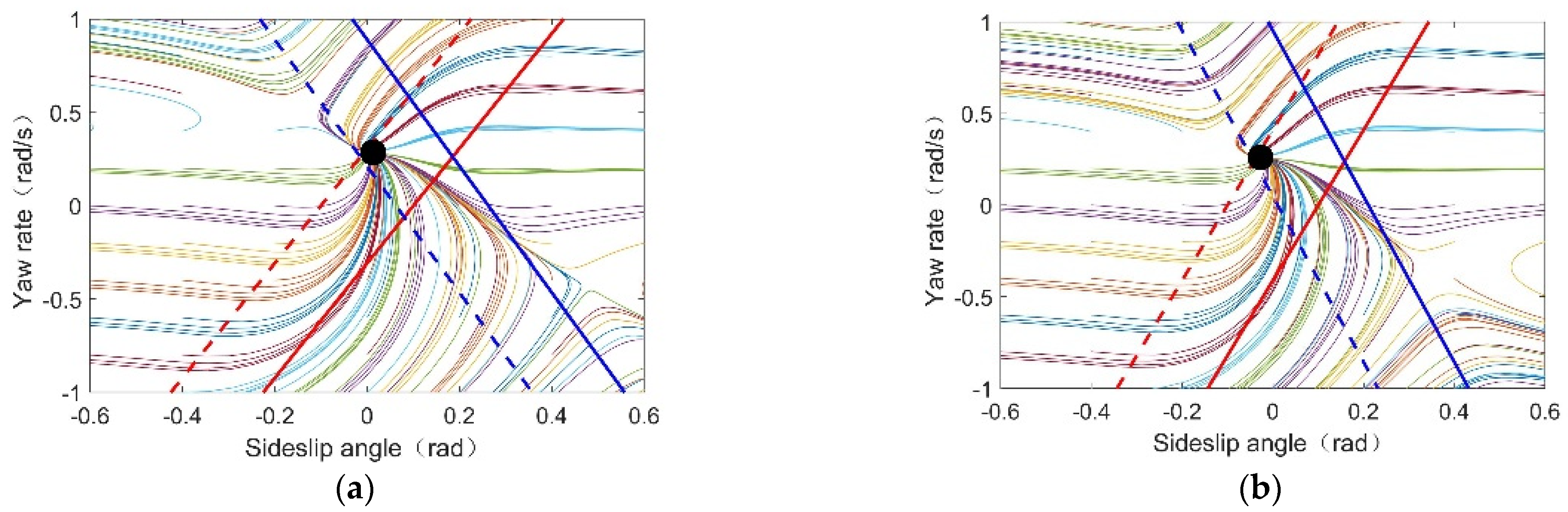
Figure 4 shows the phase plane corresponding to different steering angle inputs under the conditions of road adhesion $\mu =0.8$ and vehicle speed $v_x=20 \mathrm{m}/\mathrm{s}$. The solid circle, solid triangle, and solid diamond in the figure represent the equilibrium point, saddle point, and focal point, respectively. The black, blue, and red lines represent the yaw rate boundary, ${\alpha }_f$ boundary, and ${\alpha }_5$ boundary, respectively. It can be seen that when ${\delta }_1=0.1 \mathrm{rad}$, the vehicle equilibrium points are all within the three corresponding boundaries. As the steering angle increases, the equilibrium point gradually approaches the left saddle point. When ${\delta }_1=0.188 \mathrm{rad}$, the left saddle point coincides with the equilibrium point, and the vehicle reaches a critical stable state. At this point, the equilibrium point precisely reaches the saturation limit of ${\alpha }_5$. Note that ${\delta }_{1c}=0.188 \mathrm{rad}$ is the critical stable steering angle. When ${\delta }_1>{\delta }_{1c}$, the system will undergo bifurcation and the equilibrium point of the system will shift from a stable node to a focal point. Comparing Figure 4b,c, it can be seen that the stable node near the equilibrium point converges faster than the stable focal point. When ${\delta }_1=0.3 \mathrm{rad}$, the vehicle state oscillates around the focal point and finally stabilizes. The ${\alpha }_f$ corresponding to the stable state exceeds the saturation limit, while the fifth axle with the largest side slip angle among the rear three axles still remains within the boundary of the tire side slip angle, which is caused by the understeer characteristics of the five-axle heavy vehicle. In this case, the vehicle state is difficult to quickly converge, and such a state can also be referred to as instability for the vehicle.

Based on the above phase plane analysis, it can be seen that when the steering angle of the first axle of a multi-axle vehicle exceeds the critical stable steering angle ${\delta }_{1c}$, the vehicle will enter an unstable state. Selecting a vehicle speed range of 10 m/s~30 m/s and a road adhesion coefficient variation range of 0.1~1, the critical stable steering angle of multi-axle heavy vehicles under multiple operating conditions is calibrated based on the phase plane analysis method. The calibration results are shown in Figure 5. It can be seen that as the road adhesion coefficient decreases and the vehicle speed increases, the critical stable steering angle ${\delta }_{1c}$ gradually decreases.

The tires linear working area boundary of ${\alpha }_f$ and ${\alpha }_5$ is introduced for phase plane analysis, and the linear critical steering angle ${\delta }_{1l}$ is calibrated. The specific boundaries introduced are as follows:

$$\begin{array}{c}\left\{\begin{array}{c}\left|{\alpha }_f\right|\le \left|{\alpha }_{flin}\right|\\ \left|{\alpha }_5\right|\le \left|{\alpha }_{5lin}\right|\end{array}\right.\end{array}$$

(12)

where ${\alpha }_{2lin}$ and ${\alpha }_{5lin}$ are the lateral slip angle boundaries corresponding to the linear working area of the tire. Under the conditions of road adhesion of 0.8 and vehicle speeds of 15 m/s and 20 m/s, the linear critical steering angle analysis is performed using the phase plane method, as shown in Figure 6. It can be seen that at a speed of 15 m/s, the corresponding linear critical steering angle ${\delta }_{1l}$ is $0.203 \mathrm{rad}$; at a speed of$20 \mathrm{m}/\mathrm{s}$, the corresponding linear critical steering angle ${\delta }_{1l}$ is $0.138 \mathrm{rad}$. Based on this, the stable state of the vehicle is defined. When ${\delta }_1\in \left[-{\delta }_{1l},{\delta }_{1l}\right]$, the vehicle is in a stable state, when ${\delta }_1\in \left[-{\delta }_{1c},{\delta }_{1l}\right]\cup \left({\delta }_{1l},{\delta }_{1c}\right)$, it is in a transition state, and when ${\delta }_1\in \left(-{\delta }_{1min},-{\delta }_{1c}\right)\cup \left({\delta }_{1c},{\delta }_{1max}\right)$, it is in an unstable state.

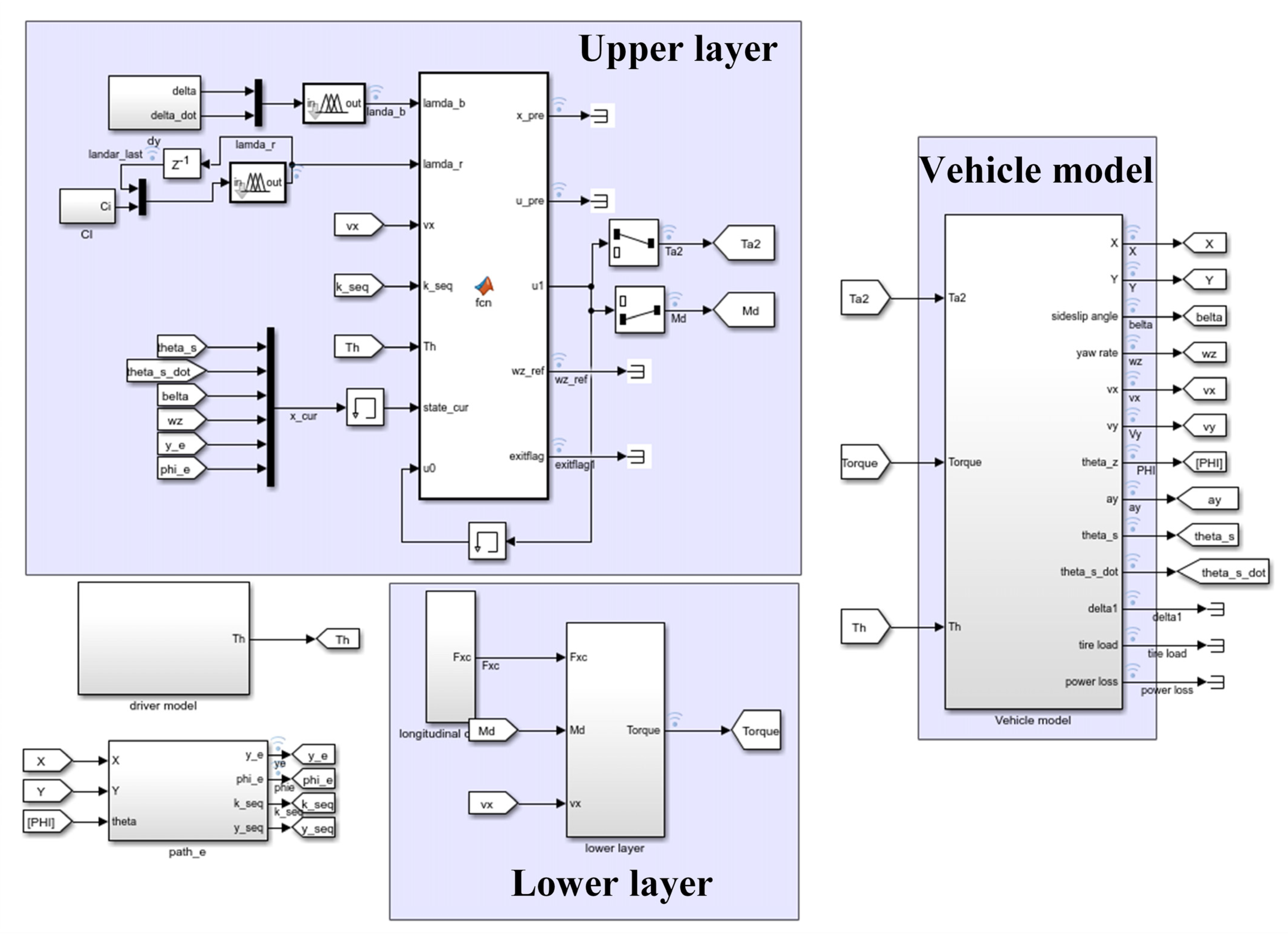
2.3. LTV-MPC Control Strategy Design

In the design of the upper layer controller, it is necessary to control the steering torque of the assisted motor and the additional yaw torque of the vehicle based on the vehicle status, the planned auxiliary obstacle avoidance path, and the driver’s input, in order to ensure that the intelligent assisted system can track the auxiliary obstacle avoidance path while avoiding human–machine conflicts and taking into account vehicle handling stability. When constructing MPC performance indicators, weight adjustment coefficients are considered to balance path tracking and vehicle handling stability. Here, the weight adjustment coefficients are obtained by mapping fuzzy logic rules with human–machine collaboration indicators, steering angle, and steering angle change rate as inputs.

Firstly, the model (9) is discretization by zero order preserving method, which is expressed as follows:

$$\begin{array}{c}\left\{\begin{array}{c}{\mathit{x}}_{k+1,t}={\mathit{A}}_{k,t}{\mathit{x}}_{k,t}+{\mathit{B}}_{k,t}{\mathit{u}}_{k,t}+{\mathit{C}}_{k,t}{\mathit{w}}_{k,t}+{\mathit{d}}_{k,t}\\ {\mathit{y}}_{k,t}={\mathit{D}}_{k,t}{\mathit{x}}_{k,t}\end{array}\right.\end{array}$$

(13)

where ${\mathit{A}}_{k,t}=e^{{\mathit{A}}_{t}T}$, ${\mathit{B}}_{k,t}={{\displaystyle \int }}_0^T{e}^{{\mathit{A}}_t\mathit{\tau }}\cdot {\mathit{B}}_{t}d\tau$, ${\mathit{C}}_{k,t}={{\displaystyle \int }}_0^T{e}^{{\mathit{A}}_t\tau }\mathit{\cdot }{\mathit{C}}_{t}d\tau$, ${\mathit{d}}_{k,t}={{\displaystyle \int }}_0^T{e}^{{\mathit{A}}_t\mathit{\tau }}\cdot {\mathit{d}}_{t}d\tau$, ${\mathit{D}}_{k,t}={\mathit{D}}_t$. $T$ is the sampling interval, and matrices ${\mathit{A}}_{k,t}$, ${\mathit{C}}_{k,t}$, and ${\mathit{d}}_{k,t}$ are calculated in real time at each control time based on the longitudinal vehicle speed $v_x$, ${\overline{C}}_i$, and ${\overline{K}}_i$. The values of $v_x$, ${\overline{C}}_i$, and ${\overline{K}}_i$ are considered to remain constant over the prediction horizon, and the driver torque $T_h$ in the measurable disturbance matrix ${\mathit{w}}_{k,t}$ is also considered constant in the prediction horizon.

The cost function $J$ of the assisted driving controller mainly consists of two parts, namely the path tracking cost $J_r$ and the handling stability cost $J_{dy}$. The cost function is specifically represented as follows:

$$\begin{array}{c}J=J_r+J_{dy}+\xi \cdot \epsilon \end{array}$$

(14)

$$\begin{array}{c}{J}_r={{\lambda }_r}^{a_r}\cdot {\displaystyle {\displaystyle \sum }_{k=1}^{N_p}}\Vert {\mathit{H}}_r\cdot {\mathit{y}}_{k,t}-{\mathit{y}}_{k,t}^{r,ref}{\Vert }_{{\mathit{Q}}_r}^2+\frac{1}{{{\lambda }_r}^{b_r}+d_r}\cdot {\displaystyle {\displaystyle \sum }_{k=1}^{N_c}}\Vert {\mathit{G}}_r\cdot u_{k,t}{\Vert }_{{\mathit{R}}_r}^2+\frac{1}{{{\lambda }_r}^{c_r}+d_r}\cdot {\displaystyle {\displaystyle \sum }_{k=1}^{N_c}}\Vert {\mathit{G}}_r\cdot \Delta u_{k,t}{\Vert }_{R_{r2}}^2\end{array}$$

(15)

$$\begin{array}{c}{J}_{dy}={\displaystyle {\displaystyle \sum }_{k=1}^{N_p}}\left({\lambda }_{\beta }\cdot \Vert {\mathit{H}}_{\beta }\cdot {\mathit{y}}_{k,t}-{\mathit{y}}_{k,t}^{\beta ,ref}{\Vert }_{{\mathit{Q}}_{\beta }}^2+\left(1-{\lambda }_{\beta }\right)\Vert {\mathit{H}}_{{\omega }_z}\cdot {\mathit{y}}_{k,t}-{\mathit{y}}_{k,t}^{{\omega }_z,ref}{\Vert }_{{\mathit{Q}}_{{\omega }_z}}^2\right)+\\ {\displaystyle {\displaystyle \sum }_{k=1}^{N_c}}\Vert {\mathit{G}}_{dy}\cdot u_{k,t}{\Vert }_{{\mathit{R}}_{dy}}^2+{\displaystyle {\displaystyle \sum }_{k=1}^{N_c}}\Vert {\mathit{G}}_{dy}\cdot \Delta u_{k,t}{\Vert }_{{\mathit{R}}_{dy2}}^2\end{array}$$

(16)

where $N_p$ and $N_c$ represent the prediction horizon and the control horizon, respectively. ${\mathit{H}}_r$, ${\mathit{H}}_{\beta }$, ${\mathit{H}}_{{\omega }_z}$, ${\mathit{G}}_r$ and ${\mathit{G}}_{dy}$ are coefficient matrices that satisfy ${\mathit{H}}_r\cdot \mathit{y}={\left[\begin{array}{cc}{y}_e& {\psi }_e\end{array}\right]}^T, {\mathit{H}}_{\beta }\cdot \mathit{y}=\beta , {\mathit{H}}_{{\omega }_z}\cdot \mathit{y}={\omega }_z, {\mathit{G}}_r\cdot u=T_{a2}, {\mathit{G}}_{dy}\cdot u=M_d$. $\Delta u$ is the control increment that satisfies $\Delta u_k=u_{k+1}-u_k$. ${\mathit{y}}_{k,t}^{r,ref}, {\mathit{y}}_{k,t}^{\beta ,ref}and {\mathit{y}}_{k,t}^{{\omega }_z,ref}$ are the reference values of the output variable. ${\mathit{Q}}_r$, ${\mathit{Q}}_{\beta }$ and ${\mathit{Q}}_{{\omega }_z}$ are the error weight matrices of the corresponding output variable. ${\mathit{R}}_r$ and ${\mathit{R}}_{dy}$ are the weight matrices of the corresponding control variable, and ${\mathit{R}}_{r2}$ and $R_{dy2}$ are the weight matrices of the corresponding control increment. ${\lambda }_r$ is the assisted driving weight adjustment coefficient, ${\lambda }_{\beta }$ is the stability weight adjustment coefficient, and their range is 0~1. $a_r~d_r$ are constants, where the purpose of $d_r$ is to ensure that the cost function is meaningful when ${\lambda }_r=0$. $\xi$ is the relaxation weight coefficient, and $\epsilon$ is the relaxation variable of the state constraint.

The weight matrices ${\mathit{Q}}_i$ and ${\mathit{R}}_i$ involved in cost function $J$ remain unchanged, and in multi-objective optimization, the coefficients ${\lambda }_r$ and ${\lambda }_{\beta }$ play a regulatory role in the cost function. The cost of path tracking $J_r$ is mainly used to adjust the effect of human–machine collaborative steering. When there is a significant human–machine conflict, the weight of path tracking is reduced, while the relevant penalties for control are increased to suppress the machine’s effort in steering for path tracking. $J_{dy}$ is used to balance and improve the dynamic performance of the vehicle. Generally, priority is given to ensuring the maneuverability of the vehicle. When the vehicle is in an unstable state, the weight of the vehicle sideslip angle error can be increased to maintain vehicle stability.

The path tracking error reference ${\mathit{y}}_{k,t}^{r,ref}={[\begin{array}{cc}{y}_{e,ref}& {\psi }_{e,ref}\end{array}]}^T$ satisfies $y_{e,ref}=0$ and ${\psi }_{e,ref}=0$. Stability control takes zero sideslip angle of the vehicle as the control objective, meeting ${\mathit{y}}_{k,t}^{\beta ,ref}={\beta }_{ref}=0$. In the process of assisting obstacle avoidance, good vehicle handling can enhance the driving experience. A steady-state reference model is used as the reference for yaw rate control, meeting ${\mathit{y}}_{k,t}^{{\omega }_z,ref}={\omega }_{z.ref}$. The reference yaw rate is represented as:

$$\begin{array}{c}{\omega }_{z,ref}=max\left(min\left(\frac{\frac{v_x}{L_e}}{K{v}_x^2+1}{\delta }_1,\frac{\mu g}{v_x}\right),-\frac{\mu g}{v_x}\right)\end{array}$$

(17)

where $K$ and $L_e$ are the stability factor and equivalent wheelbase, respectively.

In the setting of constraints, it is necessary to constrain the control variable $\mathit{u}$ and the control increment $\Delta \mathit{u}$. In the constraint of state variables, the constraints of the vehicle sideslip angle and yaw rate are satisfied ${\beta }_{max}=-{\beta }_{min}=\arctan \left(0.02 \mathsf{\mu }\mathrm{g}\right)$, ${\omega }_{z,max}=-{\omega }_{z,min}=\frac{\mu g}{v_x}$.

The optimization problem of MPC collaborative assisted driving control strategy can be summarized as follows:

$$\begin{array}{c}MinJ=J_r+J_{dy}+\xi ·\epsilon \hfill \\ st.{\mathit{x}}_{k+1,t}={\mathit{A}}_{k,t}{\mathit{x}}_{k,t}+{\mathit{B}}_{k,t}{\mathit{u}}_{k,t}+{\mathit{C}}_{k,t}{\mathit{w}}_{k,t}+{\mathit{d}}_{k,t}\hfill \\ {\mathit{y}}_{k,t}={\mathit{D}}_{k,t}{\mathit{x}}_{k,t}\hfill \\ {\mathit{u}}_{min}\le \mathit{u}\le {\mathit{u}}_{max}\hfill \\ {\mathit{u}}_{min}\le \mathit{u}\le {\mathit{u}}_{max}\hfill \\ {\mathit{x}}_{min}-\mathit{\epsilon }\le \mathit{x}\le {\mathit{x}}_{max}+\mathit{\epsilon }\hfill \end{array}$$

(18)

where ${\mathit{u}}_{min}$, ${\mathit{u}}_{max}$, $\Delta {\mathit{u}}_{min}$, $\Delta {\mathit{u}}_{max}$, ${\mathit{x}}_{min}$, and ${\mathit{x}}_{max}$ is the specific constraint matrix.

2.4. Fuzzy Collaborative Control Strategy

The fuzzy collaborative control strategy includes four input parameters, namely the human–machine cooperation index $CI$ and the assisted driving weight adjustment coefficient at the previous moment ${\lambda }_{r,last}$, the vehicle’s steering angle ${\delta }_1$ and angle change rate ${\dot{\delta }}_1$. The input variables are inferred through two fuzzy rule bases, namely human–machine conflict and handling stability, to obtain the assisted driving weight adjustment coefficient ${\lambda }_r$ and the stability weight adjustment coefficient ${\lambda }_{\beta }$, in order to achieve human–machine collaborative control and handling stability collaborative control. The following are introductions to two fuzzy control strategies.

(1)

Fuzzy strategy for human-machine collaboration

The human–machine cooperation index $CI$ consists of three parts, namely the steering torque index $C{I}_M$, the steering torque change rate index $C{I}_{\Delta M}$, and the human–machine target path consistency index $C{I}_{path}$, expressed as follows:

$$\begin{array}{c}CI=C{I}_M\cdot C{I}_{\Delta M}\cdot C{I}_{path}\end{array}$$

(19)

The definition of $C{I}_M$ is related to the torque difference between humans and machines. Under cooperative driving, the torque direction is the same, while on the contrary, the torque is opposite and conflicting. The definition of $C{I}_M$ is as follows:

$$\begin{array}{c}C{I}_M=1-\frac{\left|T_{a2}-\left(k_h+1\right)\cdot T_h\right|\cdot \left|T_h\right|}{\left(\left|{\overline{T}}_{a2}\right|+\left(k_h+1\right)\cdot \left|{\overline{T}}_h\right|\right)\cdot \left|{\overline{T}}_h\right|}\end{array}$$

(20)

where ${\overline{T}}_{a2}$ is the average value of the torque auxiliary component, and ${\overline{T}}_h$ is the average value of the driver’s output torque range.

At the same time, the direction of change in human–machine torque also reflects the cooperative state of the human–machine. The steering torque change rate index $C{I}_{\Delta M}$ is used to supplement the lack of the human–machine conflict description in $C{I}_M$, defined as:

$$\begin{array}{c}C{I}_{\Delta M}=1-\frac{\left|{\dot{T}}_{a2}-\left(k_h+1\right)\cdot {\dot{T}}_h\right|\cdot \left|T_h\right|}{\left(\left|{\overline{\dot{T}}}_{a2}\right|+\left(k_h+1\right)\cdot \left|{\overline{\dot{T}}}_h\right|\right)\cdot \left|{\overline{T}}_h\right|}\end{array}$$

(21)

In the formula, ${\dot{T}}_{a2}$ and ${\dot{T}}_h$ are the rate of change of the torque auxiliary component and the rate of change of the driver’s output torque, while ${\overline{\dot{T}}}_{a2}$ and $\overline{\dot{T}}$ are the average values of the range of torque change rates.

The human–machine target path consistency index $C{I}_{path}$ in the future can be used as one of the evaluation factors for its cooperation possibility, and the specific definition of $C{I}_{path}$ is:

$$\begin{array}{c}C{I}_{path}=1-\frac{{{\displaystyle \sum }}_{i=1}^{N_n}\left(Y_i-y_i\right)}{\left(N_n\cdot \upsilon \right)}\end{array}$$

(22)

where $Y_i$ and $y_i$ are the intelligent assistance system and the driver’s intended path point, $N_n$ is the length of the path point, and $\upsilon$ is the normalization coefficient.

The range of variation for $C{I}_M$, $C{I}_{\Delta M}$, $C{I}_{path}$, and $CI$ is $\left[0,1\right]$. When $CI$ approaches 0, it indicates a significant conflict in the willingness of human–machine behavior, while on the contrary, it indicates that the human–machine is in a highly cooperative state. The universe of the human–machine cooperation index $CI$ is $\left[0,1\right]$. The set of fuzzy language values is defined as $I_1\in \left\{\mathrm{LC},\mathrm{MLC},\mathrm{MC},\mathrm{MHC},\mathrm{HC}\right\}$, corresponding to low, medium-low, medium, medium-high, and high cooperation, respectively. The specific membership function design is shown in Figure 7a. The input variable ${\lambda }_{r,last}$ is the assisted driving weight adjustment coefficient at the previous moment, and the assisted driving weight adjustment coefficient ${\lambda }_r$ of the current moment needs to be determined based on the human–machine cooperation index $CI$ of the current moment in ${\lambda }_{r,last}$. This can ensure a smooth transition of the weight adjustment coefficient and avoid controller solution oscillation caused by weight mutation. The universe of the assisted driving weight adjustment coefficient at the previous moment ${\lambda }_{r,last}$ is $\left[0,1\right]$ and the set of fuzzy language values is defined as $I_2\in \left\{\mathrm{LA}i,\mathrm{MLA}i,\mathrm{MA}i,\mathrm{MHA}i,\mathrm{HA}i\right\}$,corresponding to low, medium-low, medium, medium-high, and high control. Figure 7b shows the membership function of ${\lambda }_{r,last}$. The universe of the assisted driving weight adjustment coefficient ${\lambda }_r$ is $\left[0,1\right]$. The set of fuzzy language values is defined as $O_1\in \left\{\mathrm{LAo},\mathrm{MLAo},\mathrm{MAo},\mathrm{MHAo},\mathrm{HAo}\right\}$, which also correspond to different levels of control permissions (low, medium-low, medium, medium-high, high) of the intelligent assisted driving system. The specific membership function design of the output is shown in Figure 7c, and the specific definition of human–machine collaboration fuzzy rules is shown in

Table 1. Human–machine collaborative fuzzy rule library.

$\mathit{C}\mathit{I}$	${\mathit{\lambda }}_{\mathit{r},\mathit{l}\mathit{a}\mathit{s}\mathit{t}}$
	$\mathbf{L}\mathbf{A}\mathit{i}$	$\mathbf{M}\mathbf{L}\mathbf{A}\mathit{i}$	$\mathbf{M}\mathbf{A}\mathit{i}$	$\mathbf{M}\mathbf{H}\mathbf{A}\mathit{i}$	$\mathbf{H}\mathbf{A}\mathit{i}$
LC	LAo	LAo	MLAo	MLAo	MAo
MLC	LAo	MLAo	MLAo	MAo	MAo
MC	MLAo	MLAo	MAo	MAo	MHAo
MHC	MLAo	MAo	MHAo	MHAo	MHAo
HC	MLAo	MAo	MHAo	MHAo	HAo

.

(2)

Collaborative fuzzy strategy for handling stability

Based on the analysis of the stable state of the vehicle, the stable state, transitional state, and unstable state of the vehicle are defined according to the steering angle ${\delta }_1$ under different operating conditions. In addition, the driving process of the vehicle is transient, so based on this, the real-time state of the vehicle is evaluated by combining the angle change rate ${\dot{\delta }}_1$. When the angle change rate is greater, the vehicle is more likely to lose stability. The universe of ${\delta }_1$ is based on the range of steering angle constraints $\left[{\delta }_{1,min},{\delta }_{1,max}\right]$ and the set of fuzzy language values are defined as $I_3\in \left\{\mathrm{NL},\mathrm{NS},\mathrm{ZO},\mathrm{PS},\mathrm{PL}\right\}$, corresponding to negative large, negative small, zero, positive small, and positive large, respectively. A road adhesion coefficient of 0.8 and a vehicle speed of 20 m/s are used as the nominal operating conditions, and the critical steering angles $\pm {\delta }_{1l,N}$ and $\pm {\delta }_{1c,N}$ are combined to divide the interval for membership function design, as shown in Figure 8a. For other operating conditions, the steering angle can be mapped to the nominal operating condition based on the obtained calibrated critical steering angle data and the principle of proportionality. ${\dot{\delta }}_1$ is the angle change rate, which represents the change of the steering angle per unit time. Its universe is $\left[{\dot{\delta }}_{1min},{\dot{\delta }}_{1max}\right]$. Based on the same nominal operating conditions, two critical angle change rates are set as $\pm {\dot{\delta }}_{1l,N}$ and $\pm {\dot{\delta }}_{1h,N}$, defined in the fuzzy language set as $I_4\in \left\{\mathrm{NL},\mathrm{NS},\mathrm{ZO},\mathrm{PS},\mathrm{PL}\right\}$, and the membership function design is shown in Figure 8b. The universe of output variable ${\lambda }_{\beta }$ is $\left[0,1\right]$, and the fuzzy language set is $O_2\in \left\{\mathrm{LSC},\mathrm{MLSC},\mathrm{MSC},\mathrm{MHSC},\mathrm{HSC}\right\}$, corresponding to low, medium-low, medium, medium-high, and high stability control, respectively. The membership function design is shown in Figure 8c.

The specific definition of fuzzy rules is shown in

Table 2. Operational stability collaborative fuzzy rule library.

${\mathit{\delta }}_1$	${\dot{\mathit{\delta }}}_1$
	NL	NS	ZO	PS	PL
NL	HSC	HSC	HSC	MHSC	MSC
NS	HSC	HSC	MHSC	MSC	MLSC
ZO	MLSC	MLSC	LSC	MLSC	MLSC
PS	MLSC	MSC	MHSC	HSC	HSC
PL	MSC	MHSC	HSC	HSC	HSC

. The general rule is that as the steering angle approaches the unstable region and the rate of steering angle change increases, the vehicle transitions from handling control to stability control, and the value of ${\lambda }_{\beta }$ gradually increases.

The fuzzy logic MAP diagram of human–machine collaboration and handling stability collaboration is shown in Figure 9. The color of the fuzzy graph corresponds to the value of the z-axis.

3. Lower-Level Torque Distribution Strategy

This section is based on the virtual control variable composed of the generalized additional yaw moment obtained by the upper layer MPC controller and the generalized longitudinal force required for longitudinal motion tracking, combined with the minimum tire load rate and minimum energy consumption for multi-objective torque allocation. The longitudinal motion control adopts the sliding mode control algorithm, which will not be repeated here. The generalized longitudinal force and additional yaw moment required by the vehicle are generated by the longitudinal force of the tire, which can be expressed as:

$$\begin{array}{c}\left\{\begin{array}{c}{F}_{xc}={\displaystyle {\displaystyle \sum }_{i=1}^2}\left(F_{xwil}\mathit{cos}{\delta }_{il}+F_{xwir}\mathit{cos}{\delta }_{ir}\right)+{\displaystyle {\displaystyle \sum }_{i=3}^5}\left(F_{xwil}+F_{xwir}\right)\\ M_d=\frac{B}{2}\left({\displaystyle {\displaystyle \sum }_{i=1}^2}\left(-F_{xwil}\mathit{cos}{\delta }_{il}+F_{xwir}\mathit{cos}{\delta }_{ir}\right)+{\displaystyle {\displaystyle \sum }_{i=3}^5}\left(-F_{xwil}+F_{xwir}\right)\right)+{\displaystyle {\displaystyle \sum }_{i=1}^2}{\displaystyle {\displaystyle \sum }_{j=l}^r}\left(L_i{F}_{xwij}\mathit{sin}{\delta }_{ij}\right)\end{array}\right.\end{array}$$

(23)

If the rolling resistance moment is ignored and it is believed that the slip rate/speed change of each tire is not significant within a finite time [19], then the longitudinal force of each wheel can be expressed as:

$$\begin{array}{c}{F}_{xwij}=\frac{T_{wij}}{R_w}=\frac{\left(T_{ij}\cdot i_0\right)}{R_w}\end{array}$$

(24)

In the formula, $i_0$ is the reduction ratio and $T_{wij}$ is the driving torque of each wheel. $T_{ij}$ is the torque output by the wheel motor.

Substitute Equation (24) into Equation (23), and based on the small angle assumption of steering angle, the formula can be simplified as:

$$\begin{array}{c}\left\{\begin{array}{c}{F}_{xc}=\frac{i_0}{R_w}\cdot {\displaystyle {\displaystyle \sum }_{i=1}^5}\left(T_{il}+T_{ir}\right)=\frac{i_0}{R_w}\cdot \left(T_{all,l}+T_{all,r}\right)\\ M_d=\frac{i_0\cdot B}{2R_w}{\displaystyle \sum _{i=1}^5}\left(-T_{il}+T_{ir}\right)=\frac{i_0\cdot B}{2R_w}\cdot \left(-T_{all,l}+T_{all,r}\right)\end{array}\right.\end{array}$$

(25)

where $T_{all,l}$ and $T_{all,r}$ are the sums of the target torque output by the left and right wheel motors of the vehicle, $B$ is the wheelbase. Once the generalized longitudinal force and additional yaw moment are determined, the total target torque of the left and right motors can be expressed as:

$$\begin{array}{c}\left\{\begin{array}{c}{T}_{all,l}=\frac{1}{2}\left(\frac{F_{xc}{R}_w}{i_0}-\frac{2M_d{R}_w}{i_{0}B}\right)\\ T_{all,r}=\frac{1}{2}\left(\frac{F_{xc}{R}_w}{i_0}+\frac{2M_d{R}_w}{i_{0}B}\right)\end{array}\right.\end{array}$$

(26)

The torque distribution will be described as a multi-objective optimization problem consisting of three optimization objectives, the first of which is to ensure that the torque corresponding to the drive motor meets the requirements of the generalized virtual control variables, which can be represented by the tracking effect of the total torque of the left and right wheel motors on the target torque $T_{all,l}$ and $T_{all,r}$, respectively. The second optimization objective is the minimum tire load rate. Finally, it is necessary to consider the optimization of the overall energy efficiency of the vehicle, that is, to maximize the operation of each wheel motor in high efficiency areas and reduce energy loss. The specific control allocation (CA) problem can be expressed as:

$$\begin{array}{c}{J}_{CA}=J_{virtual}+J_{tire}+J_{energy}\end{array}$$

(27)

where $J_{CA}$ represents the overall optimization cost of the control allocation problem, $J_{virtual}$ represents the virtual control cost, $J_{tire}$ represents the tire load rate optimization cost, and $J_{energy}$ represents the energy efficiency optimization cost. The following is a specific explanation of each cost function.

(1)

Virtual control objectives

Define an expression for virtual control based on Formula (26).

$$\begin{array}{c}{\mathit{B}}_{CA}\cdot {\mathit{u}}_T=\mathit{v}\end{array}$$

(28)

where ${\mathit{B}}_{CA}$ is the coefficient matrix, ${\mathit{u}}_T$ is the control variable, and $v$ is the virtual control objective variable, which can be obtained according to Equation (26). Meanwhile, the virtual control cost is expressed in the form of an approximation error, as follows:

$$\begin{array}{c}{J}_{virtual}={\Vert \left({\mathit{B}}_{CA}{\mathit{u}}_T-\mathit{v}\right)\Vert }_{{\mathit{P}}_1}^2\end{array}$$

(29)

where ${\mathit{P}}_1$ is the two-dimensional virtual control variable error weight matrix.

(2)

Tire load rate optimization objectives

The tire load rate can be used to describe the utilization level of the tire under different working conditions. Considering that the lateral force of each tire in the vehicle is not controlled in longitudinal torque allocation, the tire load rate can be expressed as:

$$\begin{array}{c}{\rho }_{ij}=\frac{F_{xwij}^2}{{\left(\mu F_{zwij}\right)}^2}=\frac{{\left(T_{ij}{i}_0\right)}^2}{{\left(\mu R_w{F}_{zwij}\right)}^2}\end{array}$$

(30)

When the overall tire load rate is low, it helps to improve vehicle stability. Therefore, the stability objective in control allocation is to minimize the tire load rate of each wheel, which can be expressed as:

$$\begin{array}{c}{J}_{tire}=\Vert {\mathit{B}}_s{\mathit{u}}_T{\Vert }_{{\mathit{P}}_2}^2\end{array}$$

(31)

where the coefficient matrix ${\mathit{B}}_s$ is obtained by Equation (30). ${\mathit{P}}_2$ is the stability control objective weight matrix.

(3)

Energy efficiency optimization objectives

As shown in Figure 10, there is a corresponding motor output torque $T_{ij,me}$ that satisfies the highest energy efficiency at different speeds and satisfies the external characteristics of the motor, referred to as the optimal energy efficiency point. This study combines the total demand torque on the left and right side of the heavy vehicle and the reference torque point corresponding to the optimal energy efficiency point of each motor to develop the relevant control logic to achieve the goal of energy efficiency optimization, which can avoid the problem of real-time solution due to the non-linear energy loss function introduced by energy efficiency optimization. The energy efficiency optimization cost function can be expressed as:

$$\begin{array}{c}{J}_{energy}=\Vert {\mathit{u}}_T-{\mathit{u}}_{ref}{\Vert }_{{\mathit{P}}_3}^2\end{array}$$

(32)

where ${\mathit{P}}_3$ is the weight matrix of energy efficiency optimization objectives, and ${\mathit{u}}_{ref}$ is the reference control matrix, meeting ${\mathit{P}}_3=p_3\cdot diag\left(c_{1l},c_{1r},\dots ,c_{5l},c_{5r}\right)$, ${\mathit{u}}_{ref}={\left[\begin{array}{ccccc}{T}_{1l,ref}& T_{1r,ref}& \dots & T_{5l,ref}& T_{5r,ref}\end{array}\right]}^T$. Here, $p_3$ is a constant, and the coefficient $c_{ij}$ and the reference torque $T_{ij,ref}$ are varied according to the control logic. The left and right sides of the vehicle have the same logic for optimizing the energy efficiency of the torque distribution, so the left side of the vehicle is chosen to describe the control logic for energy efficiency optimization.

Firstly, calculate the motor distribution coefficient $\varsigma$ based on the target total torque $T_{all,l}$ that needs to be allocated on the left side:

$$\begin{array}{c}\varsigma =\frac{T_{all,l}}{T_{il,me}}\end{array}$$

(33)

where $T_{all,l}$ and $T_{il,me}$ are of the same sign. When $T_{all,l}$ is a negative braking torque, the value of $T_{il,me}$ in the negative torque working area of the motor is opposite to that under driving conditions. The energy efficiency control logic is divided into two modes: priority allocation and average allocation. When $\varsigma \le 5$, the control logic belongs to the priority allocation mode, and when $\varsigma >5$, the control logic switches to the average allocation mode. Taking $2<\varsigma <3$ as an example, in order to achieve higher energy efficiency, the priority control mode is to select two motors from the five motors for torque allocation, while making them work in the high-efficiency region as much as possible. Then, select one motor to distribute the remaining torque, and the remaining motors try not to participate in torque allocation as much as possible. Considering the low utilization rate of lateral force on the tires of the middle axle of multi-axle vehicles, priority should be given to torque distribution. The specific order of torque distribution is: third axle>fourth axle>fifth axle>first axle>second axle. The relevant variables for defining the weight matrix and reference control matrix are:

$$\begin{array}{c}{c}_{1l}=1,c_{12}=1,c_{3l}=1,c_{4l}=1,c_{5l}=0.1\end{array}$$

(34)

$$\begin{array}{c}{T}_{1l,ref}=0,T_{2l,ref}=0,T_{3l,ref}=T_{3l,me},T_{4l,ref}=T_{4l,me},T_{5l,ref}=T_{5l,me}\end{array}$$

(35)

In priority allocation mode, when the allocation coefficient is other values, the weight matrix ${\mathit{P}}_3$ and reference control matrix ${\mathit{u}}_{ref}$ can be updated through this control logic. When energy efficiency optimization is in the average allocation mode, the relevant variables are defined as:

$$\begin{array}{c}{c}_{1l}=1,c_{12}=1,c_{3l}=1,c_{4l}=1,c_{5l}=1\end{array}$$

(36)

$$\begin{array}{c}{T}_{1l,ref}=T_{1l,me},T_{2l,ref}=T_{2l,me},T_{3l,ref}=T_{3l,me},T_{4l,ref}=T_{4l,me},T_{5l,ref}=T_{5l,me}\end{array}$$

(37)

Among the three torque optimization objectives, the virtual control objective has the highest priority, followed by tire load rate and energy efficiency optimization objectives that should be dynamically adjusted based on the real-time state of the vehicle. When the stability weight adjustment coefficient ${\lambda }_{\beta }$ in the upper layer multi-objective MPC controller is larger, the optimization of the tire load rate should be dominant. When ${\lambda }_{\beta }$ is smaller, energy efficiency optimization is considered before the tire load rate. Based on this principle, the optimization objectives of redefining torque distribution control are:

$$\begin{array}{c}{J}_{CA}=J_{virtual}+{\lambda }_{\beta }\cdot J_{tire}+\left(1-{\lambda }_{\beta }\right)\cdot J_{energy}\end{array}$$

(38)

At the same time, the torque output of the motor should consider the maximum torque limit and the limitation of the attachment circle.

4. Simulation and Analysis

In this section, Matlab/Simulink is used to conduct co-simulation between the strategy and the controlled vehicle model to verify the effectiveness of the proposed multi-objective cooperative control method for assisted driving. The simulation model diagram is shown in Figure 11, in which the upper and lower strategies and the controlled vehicle model are highlighted. The main parameters involved in the simulation are shown in

Table 3. Main parameters of simulation.

Parameters	Values	Units
Vehicle mass $m$	56,000	kg
Yaw inertia $I_z$	430,000	kg·m2
Distance from axle to CG$L_i$	6.9/4.5/0/2.4/4.8	m
Wheel radius $R_w$	0.59	m
Wheelbase $B$	2.6	m
Equivalent moment of inertia $J_s$	0.1	kg·m2
Equivalent damping $b_s$	0.5	Nm·s/rad
Prediction horizon $N_p$	20	-
Control horizon $N_c$	5	-
Sampling interval $T$	0.04	s
Weight ${\mathit{Q}}_r$	diag(2.8 × 107, 2 × 106)	-
Weight${\mathit{Q}}_{\beta }$ and ${\mathit{Q}}_{{\omega }_z}$	9 × 1010/3 × 108	-
Weight${\mathit{R}}_r$ and ${\mathit{R}}_{dy}$	3 × 10−3/3 × 10−6	-
Weight${\mathit{R}}_{r2}$ and ${\mathit{R}}_{dy2}$	200/1.5 × 10−4	-
Weight ${\mathit{P}}_1$	100 eye(2)	-
Weight ${\mathit{P}}_2$	5 × 108 eye(10)	-
Weight ${\mathit{P}}_3$	50 eye(10)	-

. The simulation is carried out under unstable conditions of high adhesion and low adhesion road surfaces, respectively. In the upper controller, the MPC controller with fixed weight is selected to compare with the fuzzy variable weight MPC control strategy. The driver model involved in the simulation is built with LQR strategy, and the driver’s intention to track the target path can be adjusted by weight. At the same time, the inter-axle torque allocation strategy proposed in [20] is compared with the lower torque distribution controller for verification.

4.1. High Adhesion Road Simulation Conditions in Upper Layer Steering Angle

The simulation of high-adhesion roads is conducted on roads with an adhesion coefficient of 0.8, and the longitudinal speed of the vehicle is 20 m/s. Both the driver and the intelligent assistance system have their own target paths. The driver target is to drive in a straight line, while the intelligent assistance system target is to perform dual lane change (DLC). At the same time, the driver’s willingness to control the vehicle is relatively low under this condition. The torque input of the driver in Figure 12c is maintained at a relatively low level, which results in the proposed strategy’s assisted driving weight adjustment coefficient ${\lambda }_r$ based on fuzzy rules approaching 1 (as shown in Figure 12b). At this point, the auxiliary systems under both strategies have high driving control rights, and the auxiliary component $T_{a2}$ by the steering motor has absolute control over the vehicle’s steering. As shown in Figure 12a, both of them can complete the tracking of the target path of the intelligent assistance system. In terms of vehicle dynamics control, the proposed strategy proposes a handling stability collaborative control method, which dynamically adjusts the stability weight adjustment coefficient ${\lambda }_{\beta }$ for different conditions during vehicle operation. The results are shown in Figure 12b. Based on the steering angle results in Figure 12d, it can be observed that most of the time, ${\lambda }_{\beta }$ remains at a low value, and vehicle dynamic control prioritizes vehicle handling stability. And near t = 5 s and t = 8 s, as the vehicle’s steering angle increases, there is a risk of vehicle instability, and the corresponding ${\lambda }_{\beta }$ will rapidly increase, with stability control being the dominant factor. The comparison strategy comprehensively considers the handling and stability of the vehicle. By comparing Figure 12g,h, it can be seen that the proposed strategy has a good yaw rate tracking effect by adjusting the generalized additional yaw moment $M_d$ when there is no risk of vehicle instability. To balance stability, the comparison strategy sacrifices a certain degree of yaw rate tracking performance, which is particularly evident during the first peak of the steering angle. This also makes it necessary for the comparison strategy to maintain the path tracking by increasing the steering angle input during the DLC tracking process. It can be observed from Figure 12d that the proposed strategy has smoother steering angle changes and smaller peak values compared to the comparison strategy, and the proposed strategy has better tracking performance and corresponding better driving experience. As shown in Figure 12f, although the sideslip angles of both strategies meet the stability constraints of $\left|\beta \right|\le \arctan \left(0.02 \mathsf{\mu }\mathrm{g}\right)$, it is evident that the proposed strategy has higher vehicle stability. In summary, the proposed strategy can better solve the collaborative control of vehicle handling stability.

4.2. Low Adhesion Road Simulation Conditions in Upper Layer

The simulation of low adhesion roads is conducted on roads with an adhesion coefficient of 0.4, and the longitudinal speed of the vehicle is 15 m/s. Under this simulation condition, the driver has a strong willingness to independently control the vehicle. Figure 13c shows the torque results of the intelligent assistance system and the driver. Due to the inconsistency of the target paths between the driver and the intelligent assistance system, in order to maintain tracking of the auxiliary target path, the comparison strategy is inconsistent with the direction of the driver’s efforts, resulting in significant torque conflicts. The driver needs to continuously increase the output of the steering torque $T_h$ to ensure their own steering control over the vehicle. However, when t = 3 s, the proposed strategy can calculate the human–machine cooperation index $CI$ in real-time based on the conflict caused by the torque between the human and machine and adjust the assisted driving weight adjustment coefficient ${\lambda }_r$ in a timely manner through fuzzy logic control. As shown in Figure 13b, the assisted driving weight adjustment coefficient ${\lambda }_r$ transitions smoothly from 0.97 to 0.03 in the range of 3–4 s, and the controller maximizes the transfer of control to the driver. Figure 13c shows that the torque of the driver under the comparison strategy reaches over 10 Nm, while the peak torque input of the driver under the proposed strategy control is only about 3 Nm, which can significantly reduce the operational burden of the driver and respect the driver’s intention to operate. Meanwhile, as shown in Figure 13a, it can be observed that compared to the comparison strategy, the proposed strategy can ensure that drivers with autonomous control intentions can track the target path. Until the torque conflict between the human–machine disappears and the target path returns to consistency, the assisted driving weight adjustment coefficient ${\lambda }_r$ gradually increases around t = 10 s. The intelligent assistance system regains high control until the next conflict occurs.

In addition to its advantages in resolving human–machine conflicts, the proposed strategy can still ensure the handling stability of the vehicle. Comparison strategy B and the proposed strategy are selected for comparison in terms of vehicle dynamic control. The comparison strategy B is the same as the proposed strategy in path tracking and can solve human–machine collaboration problems. In terms of vehicle dynamic control, the comparison strategy B considers fixed-weight optimization of handling stability, which is the same as the comparison strategy. Based on Figure 12b,g, it can be observed that the proposed strategy only dynamically increases the stability weight adjustment coefficient ${\lambda }_{\beta }$ around t = 5 s and t = 9 s, with the vehicle’s stability control being the main focus. At other times, it can meet the tracking requirements for the ideal reference yaw rate of the vehicle. Meanwhile, Figure 13d shows that the proposed strategy, compared to comparison strategy B, eliminates the need for the driver to significantly adjust the steering to ensure vehicle control, greatly improving the driver’s handling of the vehicle while ensuring stability. By comparing the path tracking effects of the two strategies in Figure 13a, it can be seen that the proposed strategy can assist the driver in achieving higher accuracy and more stable path tracking effects, especially during the process of returning to the original lane.

4.3. Simulation Analysis of Torque Allocation in Lower Layer

On the premise of ensuring that the control strategy in the upper layer adopts the proposed multi-objective MPC-assisted driving control algorithm, a comparative analysis of the torque allocation strategy in the lower layer is conducted, and the simulation conditions are consistent with the verification of the upper layer strategy. Figure 14 shows the torque allocation results of the proposed strategy and the comparison strategy on the left and right wheel motors of the vehicle under high adhesion conditions. Based on Figure 15, it can be observed that the two strategies have tracking errors for the virtual control variables of longitudinal force and yaw moment at around t = 5 s and t = 8 s, which is caused by the limitation of motor torque. At other times, they can basically achieve good tracking of their respective virtual control variables. At the same time, the actual tracking effects of the two strategies for generalized longitudinal force and generalized yaw moment are almost identical. Based on this, it is fair to conduct an optimization analysis involving tire load rate and driving system energy efficiency, and there will be no situation where the tracking effect is sacrificed to improve a certain performance.

Figure 16 shows a comparison of tire load rate results corresponding to two torque allocation strategies. The increase in the stability weight adjustment coefficient of the proposed strategy at t = 5 s and t = 8 s and the improvement in the tire load rate optimization weight of the proposed torque allocation strategy significantly reduces the peak load rate of each tire at the corresponding time compared to the comparison strategy. In order to compare the tire load rate results of the two strategies more intuitively, their load rate cumulative fistribution function (CFD) results are statistically analyzed separately. As shown in Figure 17, under high adhesion conditions, the proposed torque allocation strategy and the comparison strategy have a total tire load rate of less than 5.4 at 100% and 98.3% driving times, respectively. Under low adhesion conditions, the two strategies correspond to a total tire load rate of less than 5.8 at 100% and 98.5% of driving times, respectively. It can be seen that the proposed torque allocation strategy has a better optimization effect on tire load rate compared to the comparison strategy, especially in times of high steering instability, which also indicates that it has a higher tire stability margin and is conducive to stable driving of the vehicle. Figure 18 shows the power loss comparison of the drive system under two strategies. As the proposed strategy can ensure that each wheel motor operates in high efficiency region as much as possible, it can achieve lower power loss most of the time. In order to compare the energy-saving effects of the two strategies, the instantaneous power loss under two operating conditions is integrated separately. Under high adhesion conditions, the energy consumption corresponding to the proposed torque allocation strategy and the comparison strategy are 0.1401 kWh and 0.152 kWh, respectively. Under low adhesion conditions, the energy consumption is 0.0924 kWh and 0.1006 kWh, respectively. Therefore, the proposed torque allocation strategy can achieve energy-saving effects of 7.86% and 8.13%, respectively, compared to the comparison strategy.

5. Conclusions

This study proposes a hierarchical chassis multi-objective collaborative control method for human–machine collaborative obstacle avoidance conditions. In the upper layer controller, the critical steering angle and stability region of multi-axle vehicles are first analyzed using phase plane theory, and the assisted driving weight adjustment coefficient and the stability weight adjustment coefficient are solved through fuzzy control. Finally, a fuzzy collaborative control strategy for multi-performance collaborative LTV-MPC is designed to solve human–machine conflicts and vehicle stability. In the lower-layer torque allocation strategy, an energy efficiency optimization method based on optimal energy efficiency point tracking is proposed, and the stability weight adjustment coefficient was introduced to coordinate the optimization of tire load rate and energy efficiency.

Finally, simulation and verification are conducted on the proposed strategy. The simulation results show that the upper layer LTV-MPC strategy can minimize human–machine conflicts in the process of tracking target paths and improve the vehicle’s handing stability. The lower layer torque allocation strategy significantly reduces the energy consumption of the drive system compared to inter-axle torque allocation strategy, while ensuring the tracking of the target variable. On average, it can save about 8% of energy consumption under both simulation conditions and can provide a better tire load rate optimization effect.

The research can help the assisted driving vehicle coordinate to solve the multi-objective optimization problems of man–machine cooperative driving, vehicle handing stability control, and torque distribution and improve the overall performance of the vehicle chassis. In future work, we will focus on solving the problem of obstacle avoidance path planning for assisted driving and take it as the target path of the intelligent system in this study, so that the planning and control problems of intelligent assisted driving can be comprehensively solved.

References

1. Wang, W.; Li, J.; Sun, F. The obstacle avoidance assistance control of multi-axle distributed heavy vehicles. Proc. IMechE Part D J. Automob. Eng. 2022. [Google Scholar] [CrossRef]
2. Wang, W.; Na, X.; Cao, D.; Gong, J.; Xi, J.; Xing, Y.; Wang, F.Y. Decision-making in driver-automation shared control: A review and perspectives. IEEE/CAA J. Automat. Sin. 2020, 7, 1289–1307. [Google Scholar]
3. SAE Standard J3016; Taxonomy and Definitions for Terms Related to On-Road Motor Vehicle Automated Driving Systems. SAE: Warrendale, PA, USA. 2016. Available online: https://www.sae.org/standards/ (accessed on 23 April 2023).
4. Hori, Y. Future vehicle driven by electricity and control—Research on four-wheel-motored “UOT Electric March II”. IEEE Trans. Ind. Electron. 2004, 51, 954–962. [Google Scholar]
5. Lin, C.; Liang, S.; Gong, X.; Wang, B. Coordinated yaw stability control for extreme path tracking of 4WIDEVs based on predictive control. Proc. Inst. Mech. Eng. Part D J. Automob. Eng. 2022. [Google Scholar] [CrossRef]
6. Benloucif, A.; Nguyen, A.; Sentouh, C.; Popieul, J. Cooperative trajectory planning for haptic shared control between driver and automation in highway driving. IEEE Trans. Ind. Electron. 2019, 66, 9846–9857. [Google Scholar]
7. Li, M.; Cao, H.; Song, X.; Huang, Y.; Wang, J.; Huang, Z. Shared control driver assistance system based on driving intention and situation assessment. IEEE Trans. Ind. Inform. 2018, 14, 4982–4994. [Google Scholar]
8. Oufroukh, N.; Mammar, S. Integrated driver co-pilote approach for vehicle lateral control. In Proceedings of the 2014 IEEE Intelligent Vehicles Symposium Proceedings, Dearborn, MI, USA, 8–11 June 2014; pp. 1163–1168. [Google Scholar]
9. Oudainia, M.; Sentouh, C.; Nguyen, A.; Popieulm, J.C. Dynamic Conflict Mitigation for Cooperative Driving Control of Intelligent Vehicles. In Proceedings of the 2022 IEEE Intelligent Vehicles Symposium (IV), Aachen, Germany, 4–9 June 2022; pp. 1446–1452. [Google Scholar]
10. Na, X.; Cole, D. Game-Theoretic Modeling of the Steering Interaction between a Human Driver and a Vehicle Collision Avoidance Controller. IEEE Trans. Hum.-Mach. Syst. 2015, 45, 25–38. [Google Scholar]
11. Liu, H.; Liu, C.; Han, L.; Xiang, C. Handling and Stability Integrated Control of AFS and DYC for Distributed Drive Electric Vehicles Based on Risk Assessment and Prediction. IEEE Trans. Intell. Transp. Syst. 2022, 23, 23148–23163. [Google Scholar]
12. Guo, N.; Lenzo, X.; Zhang, Y.; Zou, Y.; Zhai, R.; Zhang, T. A Real-Time Nonlinear Model Predictive Controller for Yaw Motion Optimization of Distributed Drive Electric Vehicles. IEEE Trans. Veh. Technol. 2020, 69, 4935–4946. [Google Scholar]
13. Guo, N.; Zhang, X.; Zou, Y.; Du, G.; Wang, C.; Guo, L. Predictive Energy Management of Plug-in Hybrid Electric Vehicles by Real-time Optimization and Data-driven Calibration. IEEE Trans. Veh. Technol. 2021, 71, 5677–5691. [Google Scholar]
14. Liu, H.; Zhang, L.; Wang, P.; Chen, H. A Real-time NMPC Strategy for Electric Vehicle Stability Improvement Combining Torque Vectoring with Rear-wheel Steering. IEEE Trans. Transp. Electrif. 2022, 8, 3825–3835. [Google Scholar]
15. Chen, Y.; Chen, S.; Zhao, Y.; Gao, Z.; Li, C. Optimized Handling Stability Control Strategy for a Four In-Wheel Motor Independent-Drive Electric Vehicle. IEEE Access 2019, 7, 17017–17032. [Google Scholar]
16. Adeleke, O.; Li, Y.; Chen, Q.; Zhou, W.; Xu, X.; Cui, X. Torque Distribution Based on Dynamic Programming Algorithm for Four In-Wheel Motor Drive Electric Vehicle Considering Energy Efficiency Optimization. World Electr. Veh. J. 2022, 13, 181. [Google Scholar]
17. Farroni, F.; Russo, M.; Russo, R.; Terzo, M.; Timpone, F. A combined use of phase plane and handling diagram method to study the influence of tyre and vehicle characteristics on stability. Veh. Syst. Dyn. 2013, 51, 1256–1285. [Google Scholar]
18. Bobier-Tiu, C.; Beal, C.; Kegelman, J.; Hindiyeh, R.Y.; Gerdes, J.C. Vehicle control synthesis using phase portraits of planar dynamics. Veh. Syst. Dyn. 2018, 57, 1318–1337. [Google Scholar]
19. Kim, W.; Yi, K.; Lee, J. Drive control algorithm for an independent 8 in-wheel motor drive vehicle. J. Mech. Sci. Technol. 2011, 25, 1573–1581. [Google Scholar]
20. Han, Z.; Xu, N.; Chen, H.; Huang, Y.; Zhao, B. Energy-efficient control of electric vehicles based on linear quadratic regulator and phase plane analysis. Appl. Energy 2018, 213, 639–657. [Google Scholar]
Figure 1. The overall control framework.
Applsci 13 07769 g001
Figure 2. The assisted steering system model.
Applsci 13 07769 g002
Figure 3. The 2-DOF vehicle model.
Applsci 13 07769 g003
Figure 4. Schematic diagram of phase plane. (a) δ 1 = 0.1   rad . (b) δ 1 = 0.188   rad . (c) δ 1 = 0.3   rad .
Applsci 13 07769 g004
Figure 5. The critical stable steering angle δ 1 c .
Applsci 13 07769 g005
Figure 6. Schematic diagram of phase plane analysis results. (a) δ 1 = 0.203   rad . (b) δ 1 = 0.138   rad .
Applsci 13 07769 g006
Figure 7. The specific membership function design. (a) Membership function of C I .   (b) Membership function of λ r , l a s t . (c) Membership function of λ r .
Applsci 13 07769 g007
Figure 8. Design of membership function. (a) Membership function of δ 1 . (b) Membership function of δ ˙ 1 . (c) Membership function of λ β .
Applsci 13 07769 g008
Figure 9. The fuzzy logic MAP diagram. (a) Human–machine collaboration. (b) Operational stability collaboration.
Applsci 13 07769 g009
Figure 10. Motor system efficiency MAP.
Applsci 13 07769 g010
Figure 11. The simulation model diagram.
Applsci 13 07769 g011
Figure 12. Comparison of control effects for high adhesion road simulation conditions. (a) Path tracking results. (b) Weight adjustment coefficient. (c) Torque output comparison. (d) Steering angle. (e) Generalized additional yaw moment. (f) Vehicle sideslip angle. (g) The tracking effect of the proposed strategy on yaw rate. (h) The tracking effect of the comparison strategy on yaw rate.
Applsci 13 07769 g012aApplsci 13 07769 g012b
Figure 13. Comparison of control effects for low adhesion road simulation conditions. (a) Path tracking results. (b) Weight adjustment coefficient. (c) Torque output comparison. (d) Steering angle. (e) Generalized additional yaw moment. (f) Vehicle sideslip angle. (g) The tracking effect of the proposed strategy on yaw rate. (h) The tracking effect of the comparison strategy on yaw rate.
Applsci 13 07769 g013
Figure 14. The torque allocation results under high adhesion conditions. (a) Left motor torque of the proposed strategy. (b) Left motor torque of the comparison strategy. (c) Right motor torque of the proposed strategy. (d) Right motor torque of the comparison strategy.
Applsci 13 07769 g014
Figure 15. Tracking effect of virtual control targets under high adhesion conditions. (a) Generalized longitudinal force tracking results. (b) Generalized yaw moment tracking results.
Applsci 13 07769 g015
Figure 16. Tire load rate under high adhesion conditions. (a) Left tire load rate of the proposed strategy. (b) Left tire load rate of the comparison strategy. (c) Right tire load rate of the proposed strategy. (d) Right tire load rate of the comparison strategy.
Applsci 13 07769 g016aApplsci 13 07769 g016b
Figure 17. Total tire load rate CDF value. (a) High adhesion conditions. (b) Low adhesion conditions.
Applsci 13 07769 g017
Figure 18. Comparison of power losses in drive systems. (a) High adhesion conditions. (b) Low adhesion conditions.
Applsci 13 07769 g018