Abstract
Reservoir characterization on offshore fields often faces specific challenges due to limited or unevenly distributed well data. The object of this study is the North Adriatic poorly consolidated clastic reservoir characterized by high porosity. The seismic data indicate notable differences in reservoir quality spatially. The only two wells on the field drilled the best reservoir area. Seismic data, seismic reservoir characterization, and accurate integration with scarce well data were crucial. This paper demonstrates how the application of machine learning algorithms, specifically a Deep Forward Neural Network (DFNN), and the incorporation of pseudo-well data into the reservoir characterization process can improve reservoir properties prediction. The methodology involves creating different reservoir porosity and thickness scenarios using pseudo-well data, synthetic pre-stack seismic data generation, seismic inversion, and DFNN utilization to improve porosity prediction. This study also highlights the importance of lithology discrimination in the geological model to better constrain reservoir properties distribution in the entire reservoir volume. Facies probability analysis was utilized to define interdependence between litho–fluid classes established from the well data and acoustic impedance volume. Apart from the field well data, seismic inversion results, and DFNN porosity volume as main inputs, acknowledgments from the neighboring fields also had an important role.
1. Introduction
Reservoir characterization is an important process in the oil and gas industry, as it provides valuable insights into the properties of subsurface reservoirs, which are essential for optimizing oil and gas operations. Especially in offshore fields, reservoir characterization can be challenging when there is a lack of well data or when the available data are unevenly distributed. The lack of data or unevenly spatially distributed data can lead to significant uncertainties in the reservoir model and reduced accuracy in predictions of reservoir properties. Machine learning (ML) algorithms, such as neural networks (NN), can be trained to recognize the spatial relationships between data points and make predictions considering the reservoir property’s spatial variability.
Machine learning has shown great potential in improving the accuracy and efficiency of elastic parameter definition for oil and gas reservoirs.
Hampson et al. (2001) [1] presented a new method for predicting well-log properties from seismic data using a probabilistic neural network. They cross-validated results systematically using different blind well tests for each input well to ensure minimum validation error.
Malvić and Prskalo (2007) [2] applied backpropagation NN to reservoir porosity prediction of the Beničanci field, Croatia. NN was trained with three seismic attributes and 14 wells. Cvetković et al. (2009) [3] trained several NN for the lithology and saturation predictions of the Upper Pannonian and Lower Pontian sediments in the Kloštar field, Croatia. Prediction results gave excellent correlation to the input data.
Numerous artificial neural network (ANN) models based on artificial intelligence can be applied to reservoir parameter prediction. Okon et al. (2020) [4] summarized published research on ANN for reservoir porosity prediction. In recent years, several studies have investigated the application of machine learning in elastic parameter estimation. Downton and Hampson (2018) [5] presented a workflow for the distribution of reservoir density based on rock physics relationships. They created pseudo-wells and synthetic seismic gathers, which were used for building deep neural networks (DNN). Downton et al. (2020) [6] presented hybrid theory-guided data science (TGDS)-based methods for reservoir characterization. The method involves simulating numerous rock property logs based on well data statistics, followed by using rock physics theory to model the corresponding elastic response and generate synthetic seismic data through AVO modeling. A deep neural network is then trained using the simulated logs and synthetic data. Finally, the trained neural network is used to analyze real seismic data and create maps of reservoir properties.
Including seismic data in machine learning workflow allows the simultaneous prediction of synthetic well logs from seismic data sets and does not require the intervention of an interpreter [7]. Neural networks can be used for seismic waveform inversion where velocity models have a vertical resolution comparable with tomography and low-frequency FWI, as presented in [8]. Wang et al. (2019) [9] described an end-to-end deep neural network for seismic inversion, which removed dependency on wavelet estimation.
Yang, et al. (2023) [10] presented two neural network models, the PorNet model and the BlstmNet model, to predict porosity directly from pre-stack seismic data. They tested these NN models on synthetic seismic gathers and compared them to the test results.
This paper is focused on observing the elastic reservoir properties of the North Adriatic gas reservoir. Different scenarios of reservoir porosity ranges and thicknesses were created by varying the pseudo-well data, following the methodology suggested by [5,6]. Synthetic pre-stack seismic data were generated, stacked, and used in the seismic inversion process. An extensive library of input data was then utilized to train a Deep Forward Neural Network (DFNN) for porosity prediction. The DFNN proved to be an effective tool for accurately predicting porosity, and its success in modeling reservoir properties of the North Adriatic gas reservoir was demonstrated. Moreover, to have an objective comparison of the results, we modeled porosity using the same NN but only with input from two wells.
Different methods of implementation of described seismic reservoir characterization results and their integration with the well data in the geological model were tested to find the most appropriate one. The best results in terms of all relevant reservoir properties modeling were achieved by introducing lithology classification and distribution, controlled by the well data and seismic results. After the lithology model was set up satisfactorily, it was utilized to better constrain the porosity distribution based on the well data and DFNN porosity volume as main inputs.
The accuracy of porosity evaluation in terms of the accurate range of values but also the spatial distribution through the reservoir volume is crucial for reserves estimation, as it directly and indirectly affects the calculation of the volume of hydrocarbons in place and hydrocarbon resources. The direct impact is visible in reservoir pore volume calculation, but it should be considered that porosity value is also related to and, to some extent, affects fluid saturation and reservoir permeability. The approach presented in this paper has the potential to be applied to other subsurface exploration projects, providing valuable insights into the properties of hydrocarbon reservoirs.
2. Geological Settings
During the geological history, sedimentary conditions in the Adriatic Sea have changed significantly, as well as tectonic activity. The final formation of the Adriatic Sea occurred during the Holocene after the Flandrian transgression [11]. The oldest drilled rocks are Permian and Triassic, deposited on an epeiric carbonate platform on the northeastern edge of Gondwana. They are followed by intra-oceanic rocks, deposited on an isolated mega-platform, from the end of the Ladinian to the younger Lower Jurassic (Toarcian), and there are deposits of the Adriatic carbonate platform (ACP) from the Toarcian to the end of the Cretaceous [12].
At the end of the Cretaceous, the massive Adriatic carbonate platform gradually disintegrates and rises. In the Paleogene, only some parts of the Adriatic carbonate platform were flooded by the sea, and carbonate sedimentation was influenced by intense tectonic activity [12].
The Adriatic Basin is characterized by distinct depressions of varying ages that formed at different times [12] (Figure 1). The Po and South Adriatic–Albania depressions are the largest but do not have continuous borders or depositional environments throughout their geological history. This is evident from variations in sediment thicknesses, areas, and unconformities between different lithological units [13,14]. Furthermore, these depressions are mostly asymmetrical in shape. In Croatia, the depressions include the entire Dugi Otok Depression, the eastern parts of the Po and Middle Adriatic Depressions, and the northern part of the South Adriatic–Albania Depression.
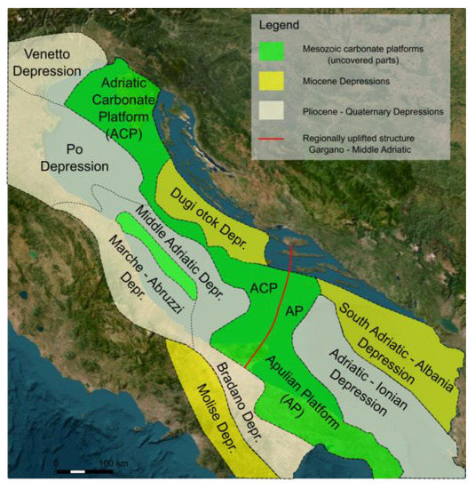
Figure 1.
Depressions in the Adriatic basin (after [13,14]).
In the area of the Northern Adriatic, Pliocene, Pleistocene, and Holocene sediments are of considerable thickness and cover the entire area, represented by limestones, clays, silts, siltstones, sandstones, and sands [13].
Based on detailed lithofacies and sequence-stratigraphic analysis, Marić Đureković (2011) [15] defined four fourth-order Plio-Pleistocene depositional sequences, Q1–Q4, and associated parasequences in the Croatian part of the North Adriatic basin. All these depositional units were detailed, including their internal architecture, depositional mechanisms, and lithofacies associations.
The Plio-Pleistocene clastic complex is significantly thicker in Italian than in the Croatian part of the Adriatic basin. Consequently, Italian lithostratigraphic nomenclature is defined in much more detail than Croatian, where the whole Paleogene to Pleistocene complex belonged to Susak Formation. Velić and Malvić (2011) [14] pointed out the need and introduced new lithostratigraphy nomenclature for the Croatian part of the basin. According to that nomenclature, Paleogene, predominantly carbonate deposits, belong to the Susak Fm., up to 500 m thick Pliocene clastics to Istra Fm., and 400–1900 m thick Pleistocene clastic complex to Ivana Fm. That division was refined by introducing Anamarija, Katarina, and Izabela members within the Ivana Fm. [16] (Figure 2).
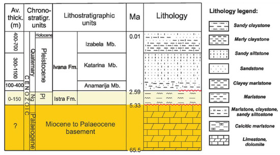
Figure 2.
Lithostratigraphic division of the Pliocene, Pleistocene, and Holocene sediments in the Croatian part of the Po Depression (after [16]).
The geological settings of the North Adriatic area are mainly the result of the interaction of Apennine fault-and-thrust-belt displacement in the northeast direction, the morphology of the foreland ramp, and the Po River delta progradation in the southeast direction [17].
The analyzed area covers the northeast part of the Po Depression and the northwest edge of the ACP foreland ramp. Depositional environments were changing frequently as a result of regional tectonic movements and eustatic sea level changes during glacials and interglacials. Generally, deep water turbidite sediments were deposited during Pliocene and Lower to Middle Pleistocene when the depositional environment gradually changed to prodelta, delta, and alluvial during Upper Pleistocene [18].
Clastic deposits in the analyzed area and depth interval, belonging to the Ivana Fm. and Izabela Mb. (Figure 2), are characterized by high porosity as a result of the depositional environment, the relative proximity of the detrital material source area, and the shallow burial depth. According to the structural and textural characteristics interpreted from image logs, analyzed reservoir rock was deposited in the river/wave-dominated delta system. Sands were delivered by distributary channels, deposited in mouth bars, and possibly reworked by waves resulting in cleaner and better-sorted sediment. Seaward from the channel/mouth bar area is the delta front and prodelta environment with deposition of silt and marl. Landward is a delta plain with distributary channels and inter-distributary areas. Described depositional settings can be compared with the modern Po Delta system [19].
3. Input Data
In this paper, we used 3D seismic data and available well data (Figure 3). Since only two wells are drilled in the researched gas field, one is used for computation pseudo-wells regarding the variation of porosity and reservoir thickness, while the second one is used as a blind well.
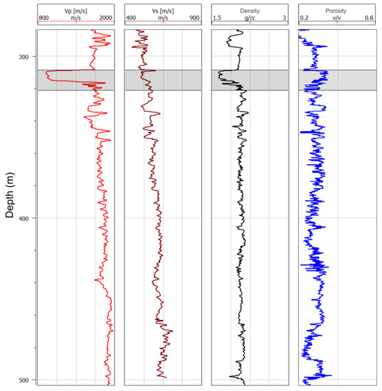
Figure 3.
Velocity, density, and porosity logs from Well A. The reservoir interval is indicated as a grey zone.
Seismic data in the case of the Adriatic basin are frequently and significantly affected by anomalies caused by gas saturation, usually at multiple levels. That makes accurate time-to-depth conversion difficult and uncertain. For the same reason, well-to-seismic data correlation is challenging, as well as direct implementation of seismic volume properties in 3D reservoir model properties in the depth domain. On the other hand, DHIs on seismic data are crucial for the interpretation of the lateral extent of gas saturation.
Well logs acquired in two wells included Gamma Ray, Resistivity, FMI, Attenuation, Density, Neutron, Sonic, and Nuclear Magnetic. Apart from Gamma Rays, the response of all other measurements is strongly affected by the gas saturation in the reservoir zone.
4. Methodology
The methodology used in this study involves seismic inversion of actual seismic data, followed by the creation of pseudo-wells with varying reservoir properties. Synthetic seismic gathers were generated from these pseudo-wells using AVO modeling techniques, and the resulting data were utilized to construct a neural network. Seismic inversion is a technique used to estimate subsurface physical properties by analyzing seismic data, which provide information about the reflectivity of geological layers. Pseudo-wells are synthetic boreholes created to simulate the subsurface properties of a reservoir. By generating synthetic seismic data from pseudo-wells with different reservoir properties, we can train a neural network to recognize patterns and relationships between the synthetic data and the subsurface properties. This methodology provides a powerful tool for analyzing subsurface structures and predicting reservoir properties.
4.1. Pre-Stack Seismic Inversion
Seismic inversion was performed to prepare validated data for the final application of the trained NN algorithm on 3D seismic data.
The pre-stack inversion is simultaneous inversion based on algorithms that derive Zp and Zs directly [20,21]. Gather analysis and transforming the input Common Depth Points (CDP) gathered from the offset domain to the incident angle domain were a preform using the defined velocity field (Figure 4). Angle Gather is stacked into partial stacks with an angle range from 0 to 10°, 10 to 20°, and 20 to 30°.
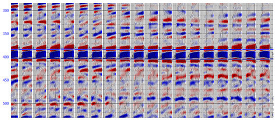
Figure 4.
Angle gathers around Well-B.
For well correlation, three angle-dependent wavelets were extracted. The cross-plot correlation was analyzed to define the relationship between Zp and Zs, and Zp and density regarding Hampson et al.’s (2005) [20] simplified mathematical formulations of the Fatti equation [22]. Such defined regression coefficients are used for inversion analysis and synthetic gather correlations with acquired CDP gather.
4.2. Pseudo-wells and Synthetic Seismic Generation
Valid elastic property distribution is always constrained by a number of objective data, more precisely, well data. For studied reservoir porosity prediction is based on artificial well catalog workflow and AVO scenarios.
Pseudo-wells are created to calculate Rock Physics properties of Well-B changing porosity and reservoir thickness (Figure 5). Porosity is varied with a range from 20% to 40%, while thickness is varied from 5 to 15 m. Reservoir mineralogy and saturation are based on Well-B petrophysical analysis. The process results in 78 pseudo-wells with associated pseudo-logs.

Figure 5.
Vp and Vs logs from several pseudo-wells created to calculate Rock Physics properties changing porosity and reservoir thickness. The reservoir interval is in grey.
AVO modeling was performed to create synthetic seismic gathers for each pseudo-well based on created logs. The synthetic gathers were calculated using the P-wave reflection coefficients obtained from the Zoeppritz equations [23] and a wavelet extracted from actual seismic data. Synthetic gathers generated from 12 pseudo-wells are shown in Figure 6.
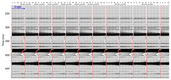
Figure 6.
AVO synthetic gathers generated from the pseudo-wells. Curves in red present Vp log.
The synthetic gathers were processed using the same methodology used for processing actual seismic data, resulting in the creation of a series of angle stacks with the same angle range. To obtain the same set of input data, pre-stack seismic inversion is performed on synthetic AVO gathers. These synthetic angle stacks were used as inputs for the neural network analysis.
4.3. Neural Network and Porosity Prediction
Neural networks are a type of machine learning algorithm that is inspired by the structure and function of the human brain, which idea is based on the work of McCullock and Pitts (1943) [24]. They consist of layers of interconnected nodes or neurons that can process and analyze data to identify patterns, make predictions, or perform other tasks.
While the concept of neural networks is based on an idealized version of how the brain works, the practical applications of this technology have shown that it can be a highly effective tool for solving real-world problems.
By connecting well and seismic data, it is possible to better define the characteristics of the reservoirs. The lateral distribution of porosity is based on the correlation between petrophysical, well, and seismic data [1]. Neural networks are used to define the correlation between input data that are not in a strictly linear relationship [3]. A multilayer neural network, a Deep Forward Neural Network (DFNN) with three hidden layers, was used (Figure 7).
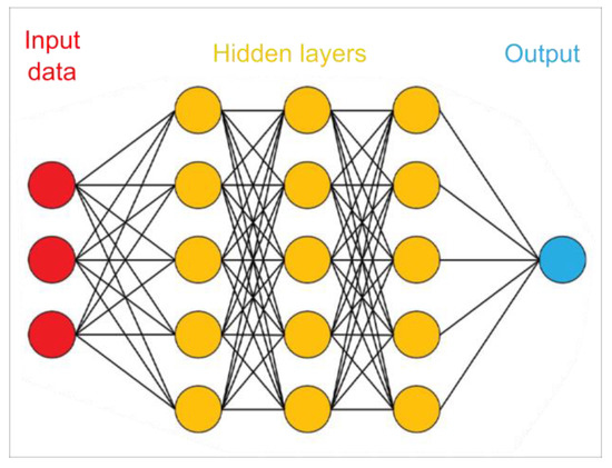
Figure 7.
Schematic example of DFNN with three hidden layers (modified after [6]).
Several published papers attempt to apply neural networks to reservoir property distribution, and research showed that DFNN has better results with petrophysical parameters [4,25,26,27].
Deep neural networks (DFNN) are a type of artificial neural network (ANN) that consists of multiple layers of interconnected artificial neurons organized in a forward propagation manner. DFNNs are often used for various tasks, such as classification, regression, and pattern recognition. DFNN consists of an input layer, multiple hidden layers, and an output layer. Each layer consists of multiple artificial neurons, also known as nodes or units. The connections between neurons are weighted, and the weights determine the strength and significance of the information transmitted between neurons. The forward propagation process of a DFNN involves passing the input data through the network, layer by layer, until the output layer is reached. Each neuron in a layer receives input from the previous layer and applies a mathematical transformation to produce an output. The output of each neuron is then passed as input to neurons in the next layer until a final output is generated. A chronological and systematic overview of the development of deep neural networks is presented by Bouwmans et al. (2019) [28].
Deep neural networks with many layers and parameters increase the risk of overfitting, characterized by small training and large validation errors. Overfitting can be reduced by increasing the amount of training data using synthetic data [20].
Pseudo-wells were used for neural network training as well as created synthetic AVO gathers, which were used as additional volume. DFNN was created with three hidden layers. Log prediction is validated using 30% of overall wells (Figure 8).
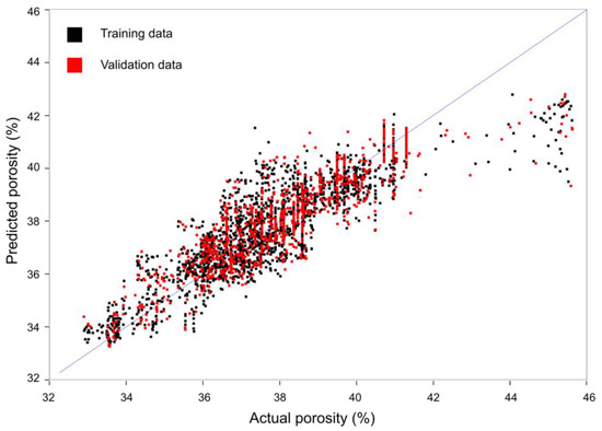
Figure 8.
DFNN validation cross-plot, which compares actual and predicted total porosity. For validation is used 30% of overall input wells.
In the final step of synthetic AVO gathers, synthetic impedance is replaced with real seismic angle stacks and impedance inversion results. Well-A is not used in this process and represents the control blind well. For the purpose of objective comparison of results, we trained the same NN but only with input from two wells and seismic inversion results from actual data.
Prior to the implementation of reservoir properties into the reservoir model, lithology discrimination was performed using an unsupervised neural network. Unsupervised neural networks employ a technique that automatically classifies input data into a specific number of classes, which are determined by the user. The network searches for patterns and trends in the input data and adjusts its function accordingly. It decides which output is most suitable for a given input and reorganizes the data to optimize its performance. The network parameters are determined by a self-organizing process that continually refines the classification results, creating a more accurate model over time. For each class, porosity is distributed based on the DFNN porosity result.
5. Seismic Reservoir Characterization Results
Pre-stack inversion resulted in 3D volumes of acoustic impedance (Zp), shear impedance (Zs), and VpVs ratio results. An inversion cross-section shows good reservoir continuity between wells Well-A and Well-B (Figure 9). Seismic interpretation indicates that the deposit has a pinch-out to the north and south and partially to the east. According to the results of the seismic inversion, the reservoir has reduced collector properties toward the east. Influence of shallower gas-bearing channels on impedance image visible as a pull-down effect is recognized on some parts of pre-stack inversion sections.
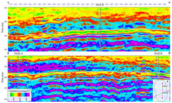
Figure 9.
Acoustic impedance seismic profiles as a result of seismic inversion on actual seismic data.
In this study, we introduce variations of porosity and thickness, which resulted in 78 pseudo-wells. This high number of reservoir property combinations exceeds reservoir property scenarios using only input well data. Porosity log prediction is validated using 30% of overall wells, and validation correlation is 89.9% using 8 attributes. Figure 10 presents the porosity prediction of seven chosen pseudo-wells compared with the input porosity log from the synthetic-well catalog.
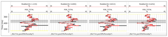
Figure 10.
Synthetic well profiles with modeled (red) and input (black) total porosity.
In the final step, synthetic AVO seismic and synthetic impedance were replaced with real seismic angle stacks and impedance inversion results. The control blind well, Well-A, was not used in this process. The total porosity map (Figure 11a) showed good reservoir continuity with clear reservoir delineation. The influence of the shallower gas-bearing channels on the results was minimized. The total porosity map (Figure 11b) based only on data from two input wells resulted in sparse porosity distribution without emphasized reservoir boundaries.
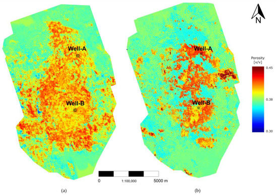
Figure 11.
Comparison of reservoir total porosity maps: (a) result of DFNN trained on synthetic catalog distribution; and (b) result of DFNN trained on input well data distribution.
6. Seismic Data Integration in the Static Reservoir Model
Just as there are different methods of seismic inversion, there are also different methods of implementing these results into a reservoir model. The selection of the method and its adaptation largely depends on the availability and quality of the input data, the type of the deposits, and the contained fluids. Numerous authors, for example, Saussus and Sams (2012) [29], advocated the approach of both facies and corresponding reservoir property distribution based on seismic reservoir characterization results. That is supported by more recent studies that are generally based on robust rock physics models. Azeem et al. (2017) [30] documented the method based on integrated petrophysical and rock physics analysis, thus improving the results of reservoir characterization. Gosh et al. (2018) [31] highlighted the importance of seismic inversion together with suitable rock physics modeling to achieve high-resolution lithofacies discrimination. Having the well data set of only two wells, both were drilled in the areas of best seismic DHIs, while at the same time, seismic showing weaker DHIs in the large area without the well data did not allow for robust rock physics modeling in this analyzed case.
Generally, for clastic reservoirs, frequent spatial variations in lithology and reservoir quality make reservoir properties assessment challenging, while gas content often masks the original rock’s elastic and physic properties. At the same time, gas-related DHIs in the seismic volume provide valuable information for spatial gas saturation boundaries definition in case of missing delineation and appraisal wells. In this presented case, as a part of lateral reservoir extent analysis, an automatic geobody extraction was performed on the Horizon probe from pre-stack Acoustic Impedance (Zp) volume for different AI windows. The range of AI values within a 50 ms thick probe is between 1500 and 5000 (m/s)(g/cm3). Based on integrated seismic and well data, values below 2700 are associated with good reservoir and gas-saturated lithologies (Figure 12).
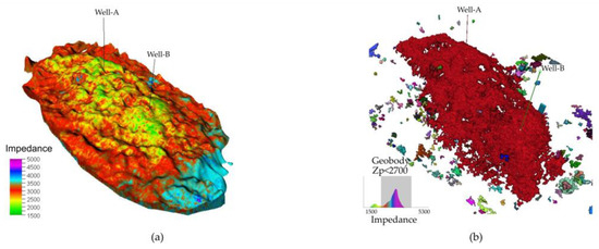
Figure 12.
Horizon probe from pre-stack Acoustic Impedance (Zp) volume covering reservoir interval (a) and extracted Reservoir geobody for Zp values lower than 2700 (m/s)(g/cm3) considered to match gas-saturated reservoir volume (b).
The purpose of seismic and well data integration and correlation is to find the geological meaning of seismic data and utilize it to propagate the rock and fluid properties in a modeled subsurface volume. The final aim is to achieve as much accuracy as possible in reservoir volume characterization with the input data set available.
In the case of the analyzed reservoir, all available well logs were strongly influenced by the gas effect, and parts of seismic volume were considered to correspond to a gas-saturated reservoir. Acquired well logs and fluid saturation profile indicate more significant variations in reservoir quality than indicated from, in general, low-contrast porosity curves (Figure 13). Based on the analog data from the neighboring fields, primary routine, and special core analysis, it was assumed to be a consequence of variations in lithology. Core data for the analyzed reservoir were not available.
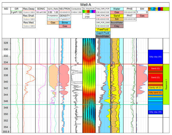
Figure 13.
Acquired well logs, Zp from seismic volume, and neural network lithology classification output.
In the previously constructed structural model, reservoir characterization workflow was adjusted to the available input data and their reliability. Seismic data, along with the well logs and analysis, were utilized to perform multi-step reservoir characterization:
- (a)
- Neural network methodology was utilized for lithology classification with the scope to differentiate reservoir quality classes and better capture reservoir quality variations in terms of reservoir parameters (Figure 13);
- (b)
- Lithology class occurrence probability analysis, derived from seismic impedance volume, previously correlated with lithology classes;
- (c)
- Probability cubes from the previous step were used for stochastic facies modeling;
- (d)
- Reservoir property modeling, including porosity, permeability, and water saturation model, was constrained by the lithology model and driven by trends from seismic reservoir characterization.
Application and comparison of the results of different classification methods for litho–fluid facies prediction were described by Aleardi and Ciabarri (2017) [32], showing the significant impact of the method applied on the resulting model. The method applied here for lithological differentiation was Unsupervised Neural Net classification based on the self-organizing process. Different input well logs and a number of output classes were tested. The final output was a result of the following input well logs: Dielectric; Deep Resistivity; FMI Conductivity; Sonic; Neutron; Density; P-impedance; and VpVs ratio. The good lithology differentiation was obtained with six classes, five of which were inside the reservoir interval and one additional representing the top reservoir seal. Due to the strong gas effect that influences the log response in all cases, within the classification process, the same lithology (e.g., sand) does not belong to the same class if it is water-saturated or gas-bearing. Therefore, each defined lithology class based on well log data, in addition to the proposed nomenclature, also contains the saturation type (G = gas; W = water), thus presenting litho–fluid classification. In that way, three gas-saturated and two water-bearing classes were defined. Based on the used neighboring gas field analogs, the main lithological difference between classes is in the ratio between the granulometric fractions that are sand, silt, and clay, and that ratio controls rock quality.
The precondition to utilize the seismic data for facies distribution is that different lithology classes are associated with reasonable seismic visibility or contrast and the possibility of establishing quantitative interdependence. The correlativity between P-impedance well log, Zp, and Lithology classes is illustrated in Figure 14. In the analyzed case, all the seismic properties that could be utilized for lithology propagation in the model are also influenced by saturation type and cannot be used solely as an indicator of lithological change. Depth-converted pre-stack seismic inversion volumes (Zp, VpVs ratio, DFNN Por) were resampled in the reservoir model and analyzed as main drivers for reservoir property spatial distribution. The initial correlation of lithology classes and input data resulted in the best correlation factor (R2 over 0.95), with P-impedance and VpVs ratio synthetic well curves.
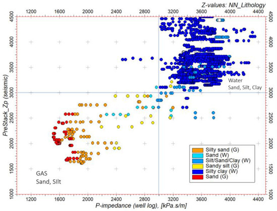
Figure 14.
Cross-plot showing a correlation between P-impedance log, Zp, and Lithology classes.
Different approaches to seismic data utilization for lithofacies propagation in the reservoir model are available. Grana et al. (2013) [33] and Babasafari et al. (2020) [34] documented good examples of facies probability prediction based on seismic inversion. Interdependence between Lithology classes and Zp here has been examined by facies probability analysis. The probability of each occurring Lithology class is driven by the histogram-based relationship with Zp as a secondary attribute (Figure 15). Generally, lower impedance values are associated with gas saturation and higher impedance with water saturation. According to the facies probability analysis, for the P-impedance values lower than 1800, the most probable Lithology class is gas-bearing sand, and for the values between 1800 and 2200, it is gas-bearing silty sand. P-impedance range between 2200 and 2800 is characteristic of the poor reservoir but still gas-bearing. There is an uncertain probability zone related to the P-impedance range 2800–3100. Water-bearing Lithology classes, according to the well and seismic data, are characterized by P-impedance values above 3100, but a clear distinction between water-bearing sand and clay inside reservoir interval based on seismic data only was not possible.
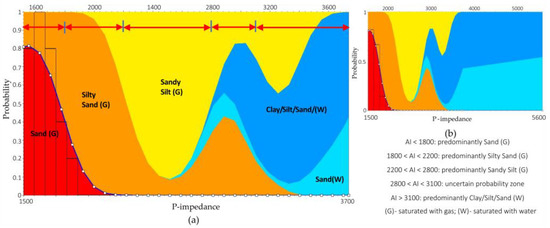
Figure 15.
Results of lithology probability analysis in dependence on P-impedance at wells (a) and for the range of Zp values in the entire reservoir interval (b).
Based on described probability analysis, a probability cube has been built for each single Lithology class representing the main input for the propagation of each Lithology class in the modeled reservoir volume. However, having five lithology classes with their probabilities increased the uncertainty in the lithology model in cases of equal probability for two or more classes. Away from well control facies, probability cubes allow great facies variations. For that reason, the lithology model has been constrained by applying two-step facies modeling, i.e., by separately modeling the gas-bearing (pay) and water-bearing (non-pay) parts of the volume in the first step and then distributing lithology classes (three in pay and two in non-pay part; (Figure 16)) constrained by tentatively named pay/non-pay model.
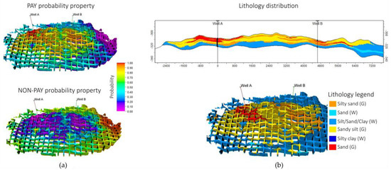
Figure 16.
Probability properties of gas-bearing (pay) and water-saturated (non-pay) Lithology classes (a) and resulting lithology distribution (b).
Reservoir properties modeling, as the last step, was constrained by the lithology model and driven by trends from seismic inversion and DFNN porosity volume (Figure 17). Based on available logs and advanced petrophysical analysis, as well as analog field data, it is expected that permeability and water saturation differ more for different lithology classes than porosity. The parameter that, according to the well log analysis, showed significant variations and impact on reservoir volumetrics and behavior is water saturation. It was concluded that all the parameters could be satisfactorily controlled by lithology classes, corresponding reservoir properties ranges, and trends from seismic inversion.
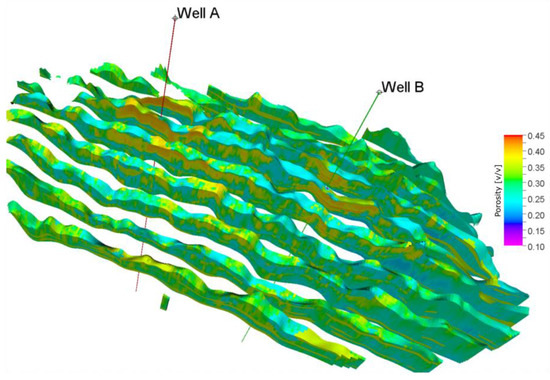
Figure 17.
Series of sections through the reservoir model showing porosity distribution.
7. Discussion
The use of synthetic pre-stack seismic data to generate a Deep Forward Neural Network (DFNN) for porosity prediction is a significant advancement in the field of subsurface exploration. This approach allows for the creation of accurate and efficient reservoir models, which can be used to optimize production and reduce exploration risk.
The success of the DFNN in accurately predicting porosity in the North Adriatic gas reservoir highlights its potential as a valuable tool in reservoir characterization. The ability to predict reservoir properties, such as porosity, is essential for optimizing production and reducing exploration risk. By accurately predicting reservoir properties, exploration, and production companies can make more informed decisions about where to drill and how to optimize production in existing wells.
The comparison of porosity prediction using input data from an extensive library versus input data from only two wells provides an objective comparison of the results. This approach demonstrates the effectiveness of the DFNN in modeling reservoir properties and the potential benefits of using a large and diverse dataset in machine learning algorithms.
The ANN models encounter limitations, such as overfitting and parameter selection, which can be overcome using different variations of activation functions, such as radial bias function instead of sigmoid [35]. Deep neural networks demand large datasets that are overcome with pseudo-well and synthetic seismic data. For complex reservoirs, proper initial reservoir set-up becomes a more crucial and critical step. This leads to a discussion about the sufficiency of varying only the thickness and porosity of the North Adriatic reservoir. To define more reliable input data for pseudo-wells and seismic, it is necessary to define a rock physics model that considers several parameters, such as deposition and mineralogical description. In the future, research should consider newly acquired well data as a result of the drilling campaign and perform sensitivity analysis of this research according to new data.
Although this methodology gives good results in reservoir characterization, we must not ignore uncertainty factors that can affect the research results. Shallow reservoirs saturated with gas, which cause a decrease in the speed of seismic waves, have a great influence on the resolution of seismic data in deeper reservoirs. According to [36,37], shallow deposits presented as valley infills also can cause imaging artifacts, such as velocity pull-downs or pull-ups.
Special attention should be paid when integrating data from different vertical resolutions. This refers to seismic versus well data but also to well-logging data of a significantly different resolution. Lithology discrimination turned out as a necessity to properly model fluid saturation and permeability, which significantly differ for overall uniform and high effective porosity values in thin, poorly consolidated deposits. However, having five litho–fluid classes with their probabilities increased the uncertainty in the lithology model in cases of equal probability for two or more classes. Away from well, control facies probability cubes allow great facies variations. Highlighted uncertainty factors may have influenced the distribution of lithological classes between wells. The two existing wells in the field targeted the best parts of the reservoir according to the seismic DHIs (Direct Hydrocarbon Indicators). In the space between the wells, seismic data indicate the gas-saturated but overall the worst reservoir. Based on lithology classification and integration with seismic data, but also considering a depositional model and acknowledgments from the neighboring fields, it was concluded that sandy silt could represent dominant lithology in that part. However, the characterization of that lithology class is relatively uncertain and partially based on analogs since it is minimally presented at well locations. The similar seismic response could also be a result of a more heterogeneous interval composed of sand and clay interlayers. To validate the results of this work, drilling additional wells and cross-checking with new data would be necessary. In the long term, the results can be confirmed or disproved by future production.
Future research in this area could focus on the application of this approach to other subsurface exploration projects and the development of more sophisticated machine learning algorithms to further improve the accuracy of reservoir property predictions. In addition, efforts could be made to incorporate additional input data, such as petrophysical and geological data, into machine learning algorithms to create more comprehensive reservoir models.
8. Conclusions
The seismic reservoir characterization results presented in this study highlight the importance and novelty of incorporating advanced techniques and data integration for improved reservoir property estimation. The use of pre-stack inversion allowed for the generation of 3D volumes of acoustic impedance, shear impedance, and VpVs ratio, providing valuable information about the subsurface properties. The seismic interpretation revealed good reservoir continuity between wells and identified the presence of gas-bearing channel and mouth-bar deposits, which had an impact on the impedance images.
One of the key contributions of this study, the first of this type in the Adriatic Basin, is the introduction of variations of porosity and thickness, resulting in a large number of reservoir property combinations. This approach goes beyond the traditional use of the input well data and expands the range of scenarios considered. The validation of porosity predictions using a subset of wells demonstrated a high correlation, highlighting the accuracy of the method. The success of the Deep Forward Neural Network (DFNN) in accurately predicting porosity in the analyzed reservoir is a significant advancement in subsurface exploration. The comparison between predictions using an extensive library versus limited well data demonstrated the effectiveness of the DFNN and the benefits of using a diverse dataset. However, this study acknowledges the limitations of the DFNN models, such as overfitting and parameter selection, which can be addressed with variations of activation functions and larger datasets.
This study also addressed the challenge of implementing seismic reservoir characterization results into a static reservoir model. Various methods were discussed, with an emphasis on facies and reservoir property distribution based on seismic data. Clastic reservoirs, such as the one analyzed in this study, are, in general, associated with significant spatial variations in lithology and reservoir quality, making the assessment of reservoir properties challenging. The incorporation of gas-related DHIs in the seismic volume provided valuable information for defining gas saturation boundaries in the absence of delineation and appraisal wells. The integration and correlation of seismic and well data aimed to extract the geological meaning of seismic data and propagate rock and fluid properties within the subsurface volume. The application of neural network methodology for litho–fluid classification allowed for better differentiation of reservoir quality classes and improved reservoir parameters capture. The lithology classes derived from the well logs classification process were correlated with seismic impedance, specifically, P-impedance, to establish quantitative interdependencies. The lithology probability analysis based on P-impedance values provided insights into both gas and water saturation and their association with different lithology classes. The resulting probability cubes formed the basis for stochastic facies modeling, which, in turn, guided the reservoir property modeling, considering porosity, permeability, and water saturation.
The integration of data with different vertical resolutions, including seismic versus well data, requires careful consideration to mitigate uncertainties. Furthermore, future research should incorporate newly acquired well data to improve the reliability of the analysis and perform sensitivity analysis accordingly.
The accuracy and detail of reservoir property estimation are significantly improved by implementing pseudo-well data, machine learning algorithms, and advanced seismic analysis techniques. The study demonstrated the effectiveness of the DFNN in modeling reservoir properties and highlighted the potential benefits of using a large and diverse dataset, especially in high-porosity sandstones. These results have implications for subsurface exploration of similar reservoirs, enabling the reduction in exploration risk and optimization of field development plans.
Author Contributions
Conceptualization, D.V.; methodology, D.V. and R.V.; software, D.V. and R.V.; validation, D.V., R.V., and Z.Č.; formal analysis, D.V. and R.V.; data curation, Z.Č.; writing—original draft preparation, D.V., R.V.; Z.Č., and V.B.; writing—review and editing, D.V., R.V.; Z.Č., and V.B.; visualization, D.V. and R.V. All authors have read and agreed to the published version of the manuscript.
Funding
This research received no external funding.
Data Availability Statement
Due to confidentiality agreements with the data owner, data cannot be made available.
Acknowledgments
The authors sincerely thank the editors and reviewers for taking the time to review this manuscript and for providing constructive feedback to improve it.
Conflicts of Interest
The authors declare no conflict of interest.
References
- Hampson, D.; Schuelke, J.; Quirein, J. Use of Multiattribute Transforms to Predict Log Properties from Seismic Data. Geophysics 2001, 66, 220–236. [Google Scholar] [CrossRef]
- Malvić, T.; Prskalo, S. Some Benefits of the Neural Approach in Porosity Prediction (Case Study from Beničanci Field). Nafta 2007, 58, 455–461. [Google Scholar]
- Cvetković, M.; Velić, J.; Malvić, T. Application of Neural Networks in Petroleum Reservoir Lithology and Saturation Prediction. Geol. Croat. 2009, 62, 115–121. [Google Scholar] [CrossRef]
- Okon, A.N.; Adewole, S.E.; Uguma, E.M. Artificial Neural Network Model for Reservoir Petrophysical Properties: Porosity, Permeability and Water Saturation Prediction. Model Earth Syst. Environ. 2021, 7, 2373–2390. [Google Scholar] [CrossRef]
- Downton, J.E.; Hampson, D.P. Deep Neural Networks to Predict Reservoir Properties from Seismic. In Geoconvetion; Geoconvention, (CEGA): Calgary, AB, Canada, 2018. [Google Scholar]
- Downton, J.E.; Collet, O.; Hampson, D.P.; Colwell, T. Theory-Guided Data Science-Based Reservoir Prediction of a North Sea Oil Field. Lead. Edge 2020, 39, 742–750. [Google Scholar] [CrossRef]
- Priezzhev, I.I.; Veeken, P.C.H.; Egorov, S.V.; Strecker, U. Direct Prediction of Petro Physical and Petroelastic Reservoir Properties from Seismic and Well-Log Data Using Nonlinear Machine Learning Algorithms. Lead. Edge 2019, 38, 949–958. [Google Scholar] [CrossRef]
- Zheng, Y.; Zhang, Q. Pre-Stack Seismic Inversion with Deep Learning. In 1st EAGE/PESGB Workshop on Machine Learning; European Association of Geoscientists and Engineers, EAGE: London, UK, 2018; Volume 2018, pp. 1–4. [Google Scholar] [CrossRef]
- Wang, K.; Bandura, L.; Bevc, D.; Cheng, S.; DiSiena, J.; Halpert, A.; Osypov, K.; Power, B.; Xu, E. End-to-End Deep Neural Network for Seismic Inversion. In SEG Technical Program Expanded Abstracts; Society of Exploration Geophysicists: San Antonio, TX, USA, 2019; pp. 4982–4986. [Google Scholar] [CrossRef]
- Yang, N.; Li, G.; Zhao, P.; Zhang, J.; Zhao, D. Porosity Prediction from Pre-Stack Seismic Data via a Data-Driven Approach. J. Appl. Geophy. 2023, 211, 104947. [Google Scholar] [CrossRef]
- Colantoni, P.; Gallignani, P.; Lenaz, R. Late Pleistocene and Holocene Evolution of the North Adriatic Continental Shelf (Italy). Mar. Geol. 1979, 33, M41–M50. [Google Scholar] [CrossRef]
- Vlahović, I.; Tišljar, J.; Velić, I.; Matičec, D. Evolution of the Adriatic Carbonate Platform: Palaeogeography, Main Events and Depositional Dynamics. Palaeogeogr. Palaeoclim. Palaeoecol. 2005, 220, 333–360. [Google Scholar] [CrossRef]
- Prelogović, E.; Kranjec, V. Geološki Razvitak Područja Jadranskog Mora (on Croatian). Pomor. Zb. 1983, 21, 387–405. [Google Scholar]
- Velić, J.; Malvić, T. Depositional Conditions during Pliocene and Pleistocene in Northern Adriatic and Possible Lithostratigraphic Division of These Rocks. Nafta 2011, 62, 25–32. [Google Scholar]
- Marić Đureković, Ž. Lithofacies and Stratigraphy of Pleistocene Deposits in North Adriatic Offshore by Using High-Resolution Well Logs. Ph.D. Thesis, University of Zagreb, Zagreb, Croatia, 2011. (In Croatian). [Google Scholar]
- Malvić, T.; Velić, J.; Cvetković, M.; Vekić, M.; Šapina, M. Određivanje Novih Pliocenskih, Pleistocenskih I Holocenskih Litostratigrafskih Jedinica u Hrvatskom Dijelu Jadrana (Priobalju). Geoadria 2015, 20, 85–108. [Google Scholar] [CrossRef]
- Ghielmi, M.; Minervini, M.; Nini, C.; Rogledi, S.; Rossi, M.; Vignolo, A. Sedimentary and Tectonic Evolution in the Eastern Po-Plain and Northern Adriatic Sea Area from Messinian to Middle Pleistocene (Italy). Rend. Lincei. 2010, 21 (Suppl. S1), 131–166. [Google Scholar] [CrossRef]
- Cattaneo, A.; Trincardi, F. The Late Quaternary Transgressive Record in the Adriatic Epicontinental Sea: Basin Widening and Facies Partitioning. In Isolated Shallow Marine Sand Bodies; Bergman, K.M., Snedden, J.W., Eds.; SEPM (Society for Sedimentary Geology): Tulsa, OK, USA, 1999; Volume 64, pp. 127–146. [Google Scholar] [CrossRef]
- Correggiari, A.; Cattaneo, A.; Trincardi, F. The Modern Po Delta System: Lobe Switching and Asymmetric Prodelta Growth. Mar. Geol. 2005, 222–223, 49–74. [Google Scholar] [CrossRef]
- Hampson, D.; Russell, B.; Bankhead, B. Simultaneous Inversion of Pre-Stack Seismic Data. In Society of Exploration Geophysicists—75th SEG International Exposition and Annual Meeting, SEG 2005; Society of Exploration Geophysicists: Houston, TX, USA, 2005; pp. 1633–1637. [Google Scholar] [CrossRef]
- Russell, B.; Hampson, D.; Bankhead, B. An Inversion Primer. CSEG Rec. 2006, 31, 96–103. [Google Scholar]
- Fatti, J.L.; Smith, G.C.; Vail, P.J.; Strauss, P.J.; Levitt, P.R. Detection of Gas in Sandstone Reservoirs Using AVO Analysis: A 3-D Seismic Case History Using the Geostack Technique. Geophysics 1994, 59, 1362–1376. [Google Scholar] [CrossRef]
- Zoeppritz, K. Über Reflexion Und Durchgang Seismischer Wellen Durch Unstetigkeitsflächen [On the Reflection and Transmission of Seismic Waves at Surfaces of Discontinuity]. Gott. Nachr. 1919, 1, 66–84. [Google Scholar]
- Mcculloch, W.; Pitts, W. A Logical Calculus of the Ideas Immanent in Nervous Activity. Bull. Math. Biophys. 1943, 5, 115–133. [Google Scholar] [CrossRef]
- Korjani, M.; Popa, A.; Grijalva, E.; Cassidy, S.; North, C. A New Approach to Reservoir Characterization Using Deep Learning Neural Networks; SPE Western Regional Meeting: Anchorage, AK, USA, 2016; pp. 23–26. [Google Scholar] [CrossRef]
- Colwell, T.; Kjøsnes, Ø. Comparative Study of Deep Feed Forward Neural Network Application for Seismic Reservoir Characterization. In First EAGE/PESGB Workshop Machine Learning; European Association of Geoscientists & Engineers: London, UK, 2018; Volume 2018, pp. 1–4. [Google Scholar] [CrossRef]
- Boonyasatphan, P.; Limpornpipat, O.; Bekti, R.P.A.; Ting, J. Facies and Reservoir Property Prediction Using Deep Feed-Forward Neural Network, a Case Study from Offshore Thailand. In Asia Petroleum Geoscience Conference and Exhibition (APGCE); European Association of Geoscientists & Engineers: Kuala Lumpur, Malaysia, 2022; Volume 2022, pp. 1–4. [Google Scholar] [CrossRef]
- Bouwmans, T.; Javed, S.; Sultana, M.; Jung, S.K. Deep Neural Network Concepts for Background Subtraction:A Systematic Review and Comparative Evaluation. Neural Netw. 2019, 117, 8–66. [Google Scholar] [CrossRef] [PubMed]
- Saussus, D.; Sams, M. Facies as the Key to Using Seismic Inversion for Modelling Reservoir Properties. First Break 2012, 30, 45–52. [Google Scholar] [CrossRef]
- Azeem, T.; Chun, W.Y.; Monalisa; Khalid, P.; Qing, L.X.; Ehsan, M.I.; Munawar, M.J.; Wei, X. An Integrated Petrophysical and Rock Physics Analysis to Improve Reservoir Characterization of Cretaceous Sand Intervals in Middle Indus Basin, Pakistan. J. Geophys. Eng. 2017, 14, 212–225. [Google Scholar] [CrossRef]
- Ghosh, D.; Babasafari, A.; Ratnam, T.; Sambo, C. New Workflow in Reservoir Modelling—Incorporating High Resolution Seismic and Rock Physics. In Proceedings of the Offshore Technology Conference Asia 2018, OTCA 2018, Kuala Lumpur, Malaysia, 20–23 March 2018. [Google Scholar] [CrossRef]
- Aleardi, M.; Ciabarri, F. Application of Different Classification Methods for Litho-Fluid Facies Prediction: A Case Study from the Offshore Nile Delta. J. Geophys. Eng. 2017, 14, 1087–1102. [Google Scholar] [CrossRef]
- Grana, D.; Paparozzi, E.; Mancini, S.; Tarchiani, C. Seismic Driven Probabilistic Classification of Reservoir Facies for Static Reservoir Modelling: A Case History in the Barents Sea. Geophys. Prospect. 2013, 61, 613–629. [Google Scholar] [CrossRef]
- Babasafari, A.A.; Ghosh, D.P.; Salim, A.M.A.; Kordi, M. Integrating Petroelastic Modeling, Stochastic Seismic Inversion, and Bayesian Probability Classification to Reduce Uncertainty of Hydrocarbon Prediction: Example from Malay Basin. Interpretation 2020, 8, SM65–SM82. [Google Scholar] [CrossRef]
- Saikia, P.; Baruah, R.D.; Singh, S.K.; Chaudhuri, P.K. Artificial Neural Networks in the Domain of Reservoir Characterization: A Review from Shallow to Deep Models. Comput. Geosci. 2020, 135, 104357. [Google Scholar] [CrossRef]
- Kristensen, T.B.; Huuse, M. Multistage Erosion and Infill of Buried Pleistocene Tunnel Valleys and Associated Seismic Velocity Effects. Geol. Soc. Spec. Publ. 2012, 368, 159–172. [Google Scholar] [CrossRef]
- Frahm, L.; Hübscher, C.; Warwel, A.; Preine, J.; Huster, H. Misinterpretation of Velocity Pull-Ups Caused by High-Velocity Infill of Tunnel Valleys in the Southern Baltic Sea. Near. Surf. Geophys. 2020, 18, 643–657. [Google Scholar] [CrossRef]


Disclaimer/Publisher’s Note: The statements, opinions and data contained in all publications are solely those of the individual author(s) and contributor(s) and not of MDPI and/or the editor(s). MDPI and/or the editor(s) disclaim responsibility for any injury to people or property resulting from any ideas, methods, instructions or products referred to in the content. |
© 2023 by the authors. Licensee MDPI, Basel, Switzerland. This article is an open access article distributed under the terms and conditions of the Creative Commons Attribution (CC BY) license (https://creativecommons.org/licenses/by/4.0/).