Hen Egg Production Forecasting: Capabilities of Machine Learning Models in Scenarios with Limited Data Sets

Abstract

To achieve a sophisticated and self-sufficient production environment that aims to optimize a particular production sequence or direction, a combination of multiple interconnected IoT devices, software, and decision-making expertise is required. This is nowadays referred to as “smart” systems and can be related to almost any field. In the case of the poultry industry, “smart” stands for automatic data gathering, in-depth processing, and decision-making support. The implementation of a smart poultry concept introduces several challenges that are production related (e.g., productivity forecasting); therefore, this study focuses on hen egg production forecasting with limited data sets. Different methods and approaches used in the poultry sector for egg production forecasting were investigated. A cross-comparison was made between different models in order to determine their applicability. The models considered include a non-linear Modified Compartmental and several machine learning (ML) models, such as, Long Short-Term Memory (LSTM), Convolutional Neural Network (CNN), XGBoost, and Random Forest (RF). Selected models used only two data sets—one for training and one for testing. Furthermore, the testing data set was significantly different than the training data, therefore setting the forecasting task to be even more challenging. The ML models had significantly more inputs that allowed them to adapt more flexibly to a changing environment in comparison with the nonlinear model that expected only one input, e.g., the week of egg production. The tests showed that the machine learning models proved to be overall more accurate than the selected nonlinear model.

1. Introduction

Smart poultry progresses firmly following the industry 3.5 and 4.0 frameworks [1,2,3]. The current trends in smart poultry are focused on monitoring parameters (by using various sensors) that affect egg/meat production, animal welfare, behaviour, and growth [4,5,6,7]. The objective of these observations is to increase the overall production’s quantity and quality. In addition, according to various poultry-related regulations and directives of the European Union [8,9,10], the maintenance of greenhouse gases should be one of the primary tasks associated with achieving the said objective. Any successful activity with observation analysis requires systematic data acquisition and processing. This can be solved by implementing a smart poultry management system. There are various commercially available solutions (such as [11,12]); however, they are designed for medium and large farms, are typically expensive, and require assistance from the management of the solution providers to be successfully used.

Our previous work includes the analysis and proposal of the smart poultry farm management system’s design [13], the development of the cyber–physical model for data acquisition and processing [14], and the evaluation of egg production process in regard to production efficiency and greenhouse gas emissions [15]. The cyber–physical model in this context is a three-component system: a set of sensors to obtain measurements, data exchange controllers that fulfil the role of an intermediary between sensors and data centre, and a data centre as an analytical hub with decision making capabilities. The term cyber–physical model can be used for almost any digitally and automatically driven production system [3,16]. Our smart poultry management system’s design focuses on decision making regarding the most appropriate feeding process while simultaneously optimising the levels of CO₂ and NH₃. The cyber–physical model was built for the proposed management system and includes three data groups—data to satisfy specific regulations, monitoring data and business-related data. In this context, data were grouped according to their sources and purposes. For example, regulations provide requirements and recommendations in the form of minimal values for environmental parameters, such as CO₂ and NH₃, whereas monitoring data encapsulates all data obtained using sensory equipment. The data of two last groups underwent complementary data fusion processing. Lastly, the implementation of the said cyber–physical model provided enough data to analyse the impact factors on the hen eggs’ production.

During the phases of the research and development of the egg production forecasting solution, the focus shifted more on evaluating and predicting egg production. Hen egg production by itself requires an in-depth understanding of the processes involved in such aspects as food formula management [17,18] and animal welfare condition management [19,20]. The egg production dynamics are typically expressed in a graphical form as a curve. According to [21,22,23], the curve applied in egg production is nonlinear and represents the number of eggs laid during a specific time frame.

In general, it is considered appropriate to apply nonlinear models in order to both analyse the historical egg production data and to predict future trends. However, based on literature analysis [4,24,25,26] and our previous work, it was concluded that the development of a smart poultry management system must incorporate multiple functional interpreters based on different types of models.

In essence, these studies lead to the necessity to assess the usefulness of generally accepted nonlinear and novel machine learning (ML) models in order to (1) determine the potential level of knowledge acquired in result of their application and (2) to incorporate the appropriate models into the framework of a developed smart poultry management system.

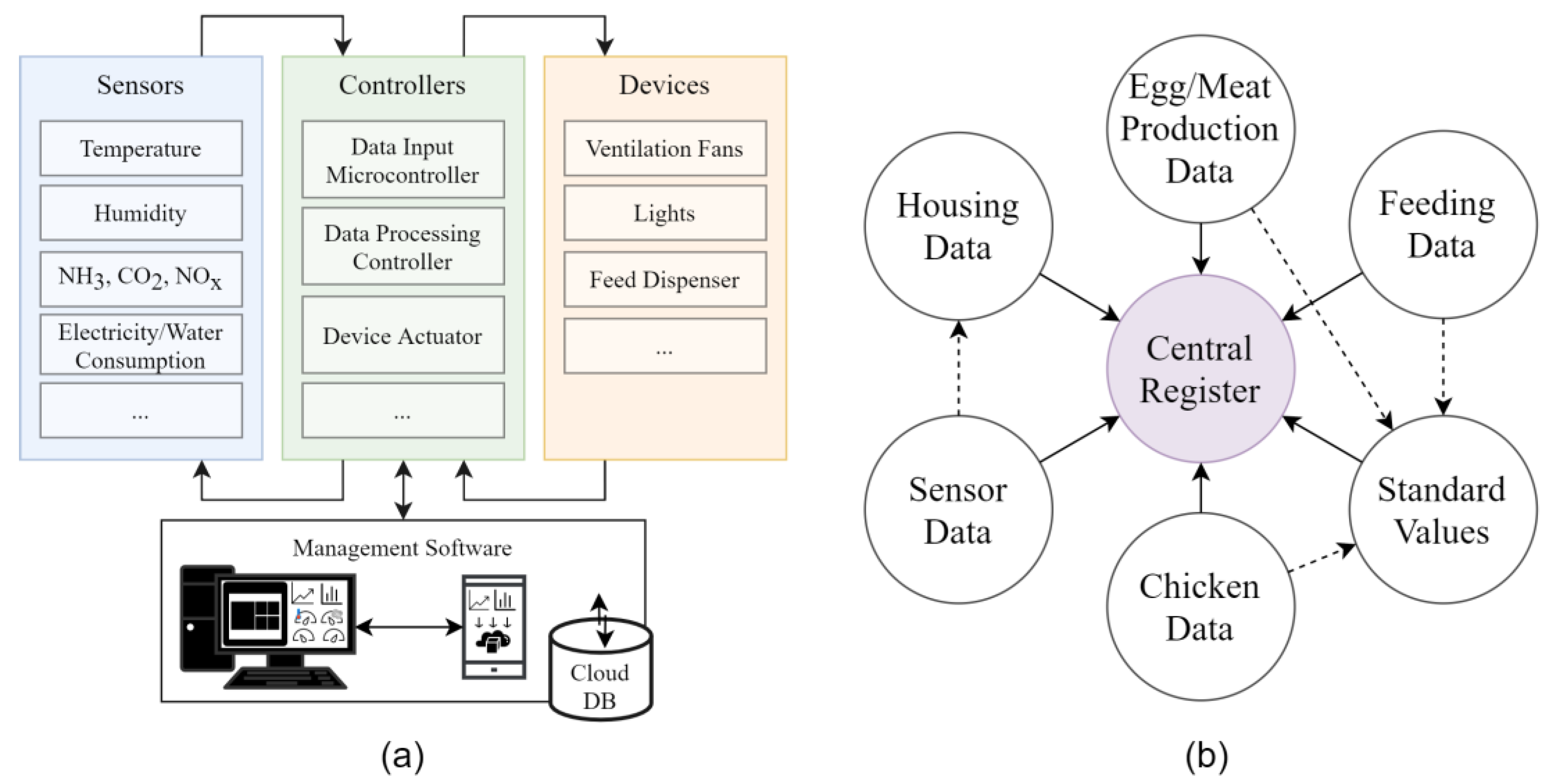
The framework itself includes: the monitoring of production-related data, a solution for data processing and analysis that incorporates adaptable database design for data storage, and a collection of models for data analysis and decision support mechanism to optimise the production processes. As stated previously—the concept of a cyber–physical model (see Figure 1a) as a basis is built upon the idea of data fusing, whereas the result of data fusion should be used for analysis of historical data and forecasting of the following short- and long-term trends in production. However, it was found [14] that current data fusion solutions on the market cannot be implemented into a framework as is, and, as a result, a multi-level data fusion approach must be taken. The architecture of the system, in turn, dictates the requirements for the number and types of such levels. Therefore, the smart poultry management system must use a data structure that (1) is sophisticated enough to encapsulate all possible data needs and (2) has a level of adaptability that is convenient for both management and farm owners. A previously proposed data structure [14] has a simplified centralised design based on one single main register and various production-related satellite tables containing parameters contributing to the final result.

The collection of multiple models is meant to provide an appropriate choice—either algorithmic, i.e., decided by the system when the data are loaded in, or manual—by a system operator—both in order to address the cases when the number of parameters between training and testing sets differ. This also partly alleviates the issues caused by imperfect data—when one model does not provide satisfactory performance and/or output, this model can be substituted with other implemented models. This assumes that all models are trained or fitted on the same data. For the purpose of encapsulating different kinds of factors and the potential results of their processing, two main types of models are included—nonlinear models and machine learning models. These types of models are further analysed in detail using scientific literature and practical experiments with real data.

The aim of this study was to cross-compare multiple models that could be used in scenarios with limited data sets to provide forecasting of egg productivity of laying hens at a sufficient level to timely point farmers towards accurate decision making.

This paper is structured as follows: first, we provide a literature review about the methods and techniques (mostly focusing on traditional nonlinear and modern machine learning models) used in the poultry industry to forecast egg production; then we describe the data sets used for practical experiments, the selected methods for hen egg production forecasting, and the training process of the selected models; after which, we describe the metrics used for evaluation and depict the results of performance cross-comparison. Finally, we discuss the obtained results and potential improvements.

2. Materials and Methods

2.1. Literature Review

Different methods can be used in order to forecast egg production rates, from models that use a small number of inputs to models that require a complex set of parameters. The further review is dedicated to nonlinear and machine learning approaches found in the literature, resulting in the selection of multiple models used for practical implementation and validation.

The application of nonlinear regression models for fitting a poultry egg production curve has been popular for several decades—a variety of nonlinear models (the incomplete gamma model by Wood [27], modified gamma model by McNally [28], model by Adams and Bell [29], Compartmental model by McMillan [30], Modified Compartmental (also called Logistic-Curvilinear [23,31]) model by Yang, Wu, and McMillan [32]) have been proposed.

Several authors have analysed and compared the traditional nonlinear models for egg production curve fitting:

• Faridi, Mottaghitalab, Rezaee, and France’s [33] research demonstrated the applicability of three Narushin–Takma models (NT1, NT2, NT3) to fit several poultry-related characteristics (such as egg production, egg weight, feed conversion ratio, etc.) of broiler breeder flocks. The performance of these models was compared with 5 others—Gompertz, Modified Compartmental, Richards, Adams–Bell, and Lokhorst. It was concluded that the NT3 model showed the best performance, measured by 4 goodness of fit criteria (MSE, R2, AIC, and BIC).
• Savegnago et al. [34] in their study selected 7 models to determine their applicability to fit weekly egg production curves in order to compare production between different selection lines of laying hens. The results of this study stated that several nonlinear models—Logistic, Persistency, Segmented Polynomial, and the Modified Compartmental model, specifically, had adequate fitting qualities and, therefore, could be applied for the egg production curve, whereas the rest of the evaluated models’, i.e., Compartmental (I and II) and McNally, performances were lacking in comparison.
• A. Safari-Aliqiarloo et al. [23] compared three nonlinear models (Compartmental, Modified Compartmental and Adams–Bell) with an Artificial Neural Network approach to fit the egg production curve of broiler breeders. Based on the evaluation criteria, the authors concluded that the ANN model had the best performance, but the Modified Compartmental model outperformed the rest in fitting the egg production curve between the selected traditional nonlinear models. This also increased the credibility of results published by Savegnago et al. [34].
• Görgülü and Akilli [21] in their study analysed the performance of four traditional nonlinear regression models (Adams–Bell, Compartmental, McNally, and Logistic model [35] together with the least square support vector machine (LSSVM) model). It was concluded that LSSVM had the best performance followed by the Adams–Bell model from the selected nonlinear model category, but its performance was better only by a narrow margin, and, as stated by the authors, all of the tested models fit the laying hens’ production curve quite well.
• Emam [36] compared the performance of four nonlinear models (Wood, McNally, Compartmental, Modified Compartmental) focusing on how well they fit the production curve of Fayoumi layers. The results of the study suggested that the Modified Compartmental model proved to have the best fit.
• Morales-Suárez et al. [18] in their research investigated the effects of different diets (focusing on variation in concentrations of three essential amino acids) on egg production of laying hens. To evaluate the egg production, authors applied three groups of models—traditional nonlinear models (Adams–Bell, McNally, Logistic, Compartmental, Modified Compartmental, Modified Gompertz, Modified Logistic), multivariate polynomial models (second and third order), and ANN models (with feed-forward and cascade-forward architectures). Based on the evaluation criteria, overall, the ANN outperformed all models. Relating to the group of nonlinear regression models, the authors stated that these models all fit the production curve well, but the Modified Logistic model had the highest goodness-of-fit scores.
• Sharifi, Patil, Yadav, and Bangar [37] compared 8 models (Logistic, Morgqan Mercer Flodin, Polynomial Fit, Rational Function, Sinusoidal Fit, Quadratic Fit, Gompertz function, Modified Compartmental) in respect to how well these models fit the egg production and egg weight curves of laying hens. The evaluation showed that Rational Function, Modified Compartmental, Sinusoidal Fit, and Polynomial Fit models performed the best in fitting the egg production.

It should be emphasised that these nonlinear models were meant to process only one factor, i.e., the age of birds (or the week of laying) as input, and to base the egg productivity completely on it. While this meant that models were applicable in cases where only one factor was available, it also revealed the limitations these models had—there was no adaptability to environmental changes. The environment was determined by such factors as outside and inside temperature, humidity, CO₂ and NH₃ concentration, air ventilation, etc. These factors could also influence egg production, either individually or in combination [38].

However, often, due to the inability to monitor all of these parameters as a complex system, only some of them are available. Therefore, the models that can make use of different parameter combinations should be assessed, similar to the models within the machine learning (ML) field.

Advances in the artificial intelligence (AI) field have led to the development of several ML models that possess nonlinearity and can also be used to forecast egg production and identify production-related problems in a timely manner. Some of the applications of the ML models in the poultry industry are described in the following studies:

• Morales, Cebrián, Fernandez-Blanco, and Sierra [39] in their study tested an SVM model with the aim to timely detect problems in egg production. The model’s accuracy was high (≈0.985) when predicting problems a day in advance.
• An ANN approach to detect early problems in egg production was presented in [40] research. In comparison with the SVM model, the ANN technique proved to be very accurate as well when predicting egg production problems a day in advance. In addition, it showed improvement in several performance evaluation metrics in comparison with the LSSVM model.
• Ahmad [4] in his research compared three different ANN architectures and traditional models for egg production forecasting. From the results of the experiment, the author concluded that the ANN models outperformed the traditional nonlinear models.

In retrospect, the results of these studies, in addition to the semi-related works [18,21,23], concluded that AI techniques were viable for application in egg production forecasting and could also lead to performance improvements (measured by several goodness-of-fit criteria) when compared to traditional, nonlinear models.

Based on the literature review on the application of nonlinear models in the poultry industry, the Modified Compartmental model’s performance proved to be consistently adequate for egg production evaluation, and it used a relatively small number of parameters that could be biologically and mathematically interpreted [32]. Therefore, the Modified Compartmental model was selected for practical experiments. From the ML group, several models were chosen since their performance stood out, as reported by several articles (described in previous chapter). For the purpose of this research, the following models (including both models previously reported by other authors and those that have not been used in egg production forecasting) were selected:

• Long Short-Term Memory (LSTM)—is a model based on recurrent neural network that has been used in precision agriculture [41] and, regarding poultry industry, for laying rate prediction [42] as well.
• Convolutional Neural Network (CNN)—is a deep learning architecture. In poultry, it has been applied with the aim to detect and classify eggs [43].
• Random Forest (RF)—a technique that generates a single model based on a combination of multiple decision trees [44]. The usage of RF for egg weight prediction is described in [2].
• XGBoost—a “tree boosting system” [45] based on decision trees and the gradient boosting approach. This model was used for feature selection in order to predict the laying rate of waterfowl [42].

The comparison and evaluation between the Modified Compartmental model and the ML models is covered in Section 3.

2.2. Development of Egg Production Forecasting Models

One of the Baltic farms was used as the location for sensor installation and integration of the developed smart poultry management system. Due to privacy and market competition concerns, the name and location of this particular farm is not specified. The laying egg production data for model comparison and evaluation were gathered from layer house, where hens (Lochman brown breed) were kept in enriched battery cages. The laying house used a belt-type manure removal system that was operated daily. The laying hens were moved to the battery cages at 16 weeks of age and were kept until 80–90 weeks of age. At 20 weeks of age, the hens started to lay eggs. The daily egg production was calculated as the ratio of the total number of eggs produced in a day to the total number of hens on that day [15].

Due to the nature of data availability, data sets were limited and for this research, egg production data for a 61-week period (data collected from 22 November 2019 to 9 February 2021) were used for model training, and a 46-week period (data collected from 23 March 2021 to 3 March 2022) of production data was used for testing (see Figure 2). The test data set was noticeably different from the one used for training and also from the usual egg production rate pattern. The reasons for such differences, according to the information provided by the farmers, could be explained by inconsistencies in data input management—whereas the number of gathered eggs was counted automatically, and the final value was inputted manually. This could be performed multiple times per day or not performed at all, for example, on weekdays or due to technical reasons. The training and testing sets, i.e., how they were split, differed for nonlinear and ML-based models and are described further.

During the egg laying periods, various types of poultry- and environment-related data were recorded, providing information about microclimate (temperature, humidity, CO₂, NH₃) and also data about bird feeding (water and feed consumption and their compositions, i.e., macro/micronutrients and microelements). The sensors for temperature and humidity monitoring were placed at the centre of the henhouse. The CO₂ (IR-2 sensor, GDS Technologies Garforth, Leeds, UK) and NH₃ (NH₃/MR-100 sensor, Membrapor AG, Wallisellen, Switzerland) concentrations were measured continuously every 10 min, but the average values were calculated each hour afterwards [15].

The winsorization technique was applied to deal with outliers in the collected data. In order to guarantee that vital information was kept in the dataset, 99% winsorization was applied, meaning that all the values below 1 percentile were set to 1 percentile, and all the values above the 99th percentile—to 99th percentile.

The environmental and feeding data for 1st and 2nd production cycle in a laying house with enriched battery cages are depicted in Figure 3.

2.3. Structure and Training of Selected Models

2.3.1. Modified Compartmental (Nonlinear)

The selected Modified Compartmental model [32] could be expressed mathematically by the following Equation (1):

y(t) = (ae^−bt)/[(1 + e^−c(t−d))],

(1)

where:

y_t—egg production rate at t weeks of laying;

a—scale parameter;

b—rate of production decrease after the peak;

t—the number of weeks laying;

c—the reciprocal indicator of the variation in the sexual maturity;

d—the mean age of the hens at sexual maturity.

The values of these parameters were then determined/evaluated by using a suitable computational approach (described in Section 3).

2.3.2. Machine Learning Models (LSTM, CNN, XGBoost, RF)

The selected ML models were built using Keras framework [46] (LSTM and CNN) and scikit-learn library [47] (RF and XGBoost). The models were tuned (hyperparameter selection) by using library extensions, such as keras-tuner and sklearn.model_selection. There were no modifications made to the selected ML models regarding their base architectures. The models were compared by varying hyperparameter values of each model. In order to find the best hyperparameter configuration, the LSTM and CNN models were tuned using the Hyperband algorithm [38], but the decision tree-based models—using Random Search [48]. The search spaces of the hyperparameters for each model are shown in

Table 1. Hyperparameters and their considered values for LSTM model.

Hyperparameter	Range of Considered Values
Input size	32, 48, 64, 80, 96, 112, 128
Dropout rate	0, 0.1, 0.2, 0.3, 0.4, 0.5
Optimizer	Adam
Learning rate	0.01, 0.001, 0.0001
Activation function	ReLU, sigmoid
Early stopping patience	10
Loss function	Mean Squared Error

,

Table 2. Hyperparameters and their considered values for CNN model.

Hyperparameter	Range of Considered Values
Filter size	32, 48, 64, 80, 96, 112, 128
Kernel size	2, 3, 5
Max Pooling size	2
Activation function	ReLU, sigmoid
Early stopping patience	10
Loss function	Mean Squared Error

,

Table 3. Hyperparameters and their considered values for XGBoost model.

Hyperparameter	Range of Considered Values
Max depth	3, 6, 10
Learning rate	0.01, 0.05, 0.1
Number of estimators	100, 500, 1000
Colsample bytree	0.3, 0.7

and

Table 4. Hyperparameters and their considered values for RF model.

Hyperparameter	Range of Considered Values
Bootstrap	True
Max depth	90, 100, 110
Min samples leaf	4, 5, 6
Min samples split	8, 10, 12
Number of estimators	100, 500, 1000

.

Early stopping technique (with a patience value 10) was used for LSTM and CNN models to potentially decrease the overfitting problem. The early stopping was also used in XGBoost hyperparameter search and training phase but the cross-validation technique in the RF case.

Refer to Appendix A for the summarised results regarding sliding window sizes and the best hyperparameter values.

The training of the models was performed using factors that were monitored daily in the poultry farm and production-related data with varying input sequence lengths, e.g., using the sliding window approach. When using such a technique, an important step is to determine the size of the window, as this defines the additional requirement for model input—the number of past productivity values, e.g., egg production in this case. If a sliding window of size 1 is chosen, it means the inputs require production data from the previous day. During the initial development stage, multiple feature selection approaches were considered, and it was determined that forward feature selection would be appropriate for usage for general ML algorithms based on the data obtained from the farm.

The selected ML models were trained on the first production cycle (that was further split into 90% train and 10% validation set in order to avoid data leakage [49] and overfitting problems [50]) and tested on the second production cycle to forecast productivity for the next day. The models’ input was formed from 12 parameters (see Figure 4) (and, additionally, the historical production data depending on the sliding window size).

2.3.3. Evaluation Metrics

Performances of the models were evaluated by different statistical criteria (see

Table 5. Criteria used for model evaluation.

Criteria	Equation
Mean Squared Error	$MSE=\frac{1}{n}{\displaystyle {\displaystyle \sum }_{i=1}^n}{\left(y_i-{\hat{\mathrm{y}}}_i\right)}^2$
Mean Absolute Percentage Error	$MAPE=\frac{100}{n}{\displaystyle {\displaystyle \sum }_{i=1}^n}\frac{\left|y_i-{\hat{\mathrm{y}}}_i\right|}{y_i}$
Root Mean Squared Percentage Error	$RMSPE=100\sqrt{\frac{1}{n}{\displaystyle {\displaystyle \sum }_{i=1}^n}{\left(\frac{y_i-{\hat{\mathrm{y}}}_i}{y_i}\right)}^2}$

where: y_i—observed value; ŷ_i—predicted value; n—number of records.

): Mean Squared Error (MSE), Mean Absolute Percentage Error (MAPE), and Root Mean Squared Percentage Error (RMSPE). The lower the value (error) of the criteria, the better the model fit the data.

3. Results

The parameters (see

Table 6. The estimated parameter values of Modified Compartmental model.

Parameter	Estimate	Std. Error	T Value	Pr (>|t|)
a	0.13099	0.01316	9.954	4.45 × 10−14 ***
b	−0.90414	0.03927	−23.024	<2 × 10−16 ***
d	2.24435	0.04658	48.182	<2 × 10−16 ***
c	−0.90766	0.03923	−23.139	<2 × 10−16 ***

) of the Modified Compartmental model were estimated using R programming language [51] to fit the egg production curve (1st cycle). From Table 6, all parameters are significant (p < 0.001, represented with three ’*’ in the last column of the table) and are applicable for this forecasting task.

The model parameters then can be filled with the estimated values (2), where the only input parameter is t, representing the number of weeks laying:

ŷ(t) = 0.13099e^{−(−0.90414)t}/(1 + e^{−(−0.90766)(t−2.24435)}),

(2)

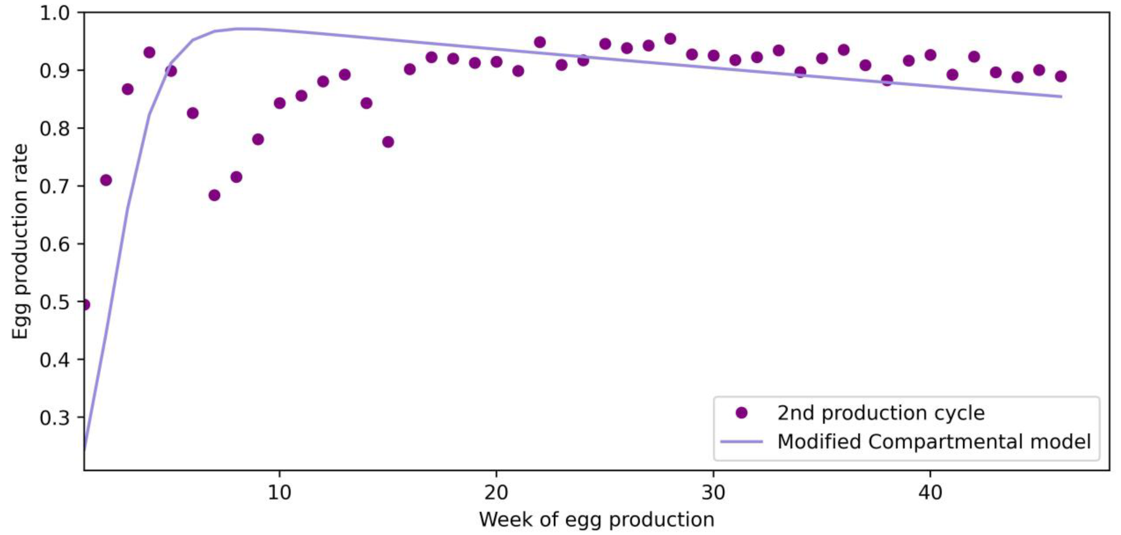
The fitted curve on the test egg production data set using the Modified Compartmental model can be seen in Figure 5.

As Figure 5 shows, the result of the model shows only the trend in the production rate, based on the previously trained data, but does not incorporate input values that could influence the prediction and point to potential problems. This production cycle demonstrates that it is not enough to base conclusions only on the week of egg production alone to achieve high accuracy, rather it allows the farmers to see the deviations from the trend.

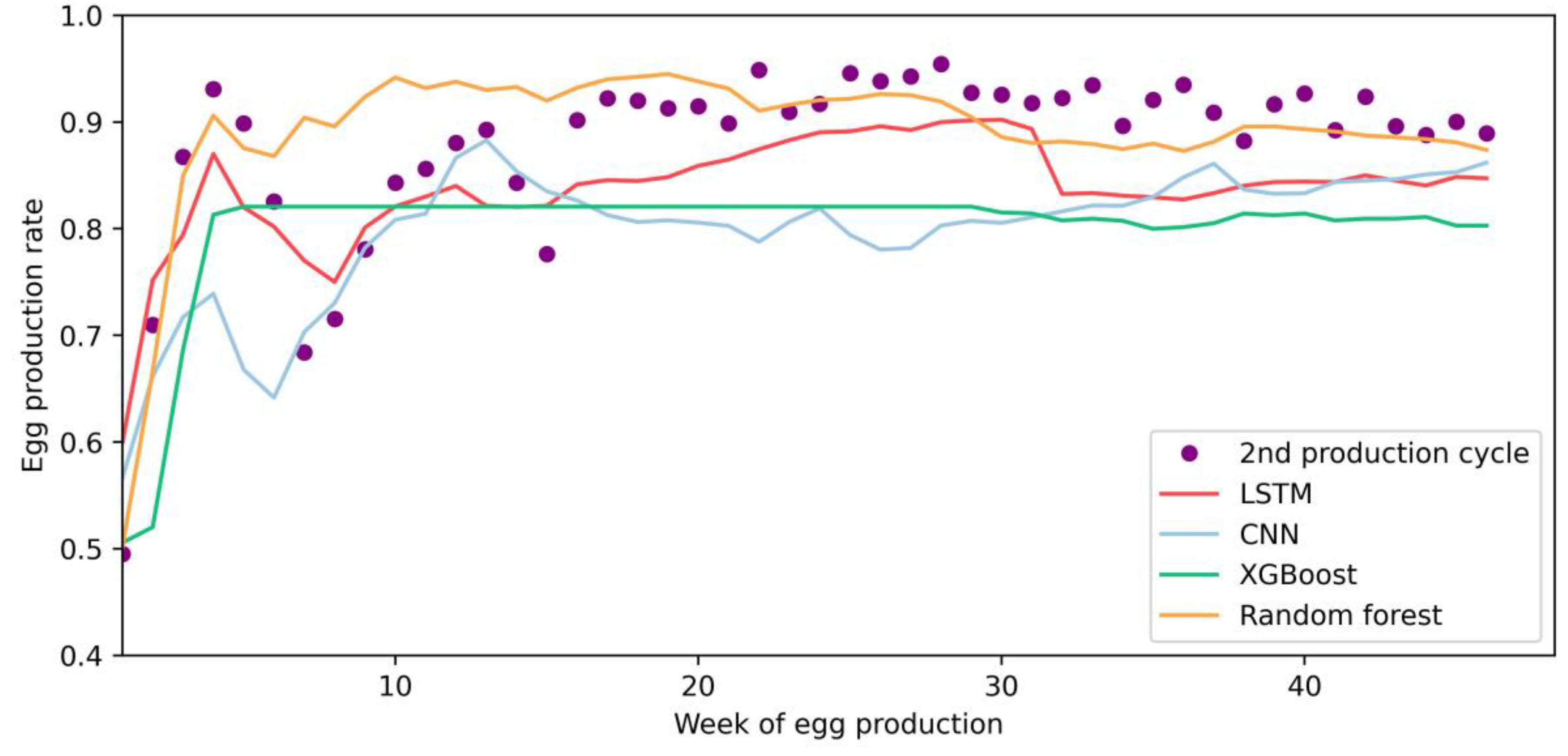
The ML model’s results and observed egg production rate with a sliding window of size two are depicted in Figure 6.

The ML models tended to follow an abnormal decrease in production (see Figure 6), thus indicating their ability to adjust to these kinds of situations. The possible reasons for the egg production variations in the 2nd production cycle were described in Section 3. Although further data inspection showed that the environmental factors did not change dramatically to have an impact on production decrease, the models forecasted the drop, due to the fact that the previous day (depending on the sliding window size) production data served as inputs.

Regarding the ML models, several window sizes were tested to determine the one that provided best prediction results. The window sizes of 1, 2, 3, 5, 7, and 14 were considered. The results of model performance per different window sizes to predict egg production for the next day are presented in

Table 7. Machine learning model performance by different sliding window sizes.

Windows Size	Error Metric	LSTM	CNN	XGBoost	RF
1	MSE	1.710	4.111	1.225	0.944
1	MAPE	13.909	14.224	9.994	6.907
1	RMSPE	15.439	16.258	11.708	10.242
2	MSE	0.272	1.884	1.060	0.726
2	MAPE	5.390	15.200	10.272	6.331
2	RMSPE	7.751	18.314	12.178	9.284
3	MSE	0.203	1.384	0.877	0.664
3	MAPE	6.501	39.319	9.086	6.158
3	RMSPE	8.828	39.993	10.875	9.110
5	MSE	0.358	0.843	0.767	0.604
5	MAPE	6.218	13.479	7.415	6.077
5	RMSPE	8.781	15.537	9.223	9.016
7	MSE	0.198	0.443	0.863	0.546
7	MAPE	5.484	13.300	9.619	6.188
7	RMSPE	7.845	14.555	11.350	9.168
14	MSE	0.153	0.308	0.719	0.453
14	MAPE	6.433	6.633	6.114	6.273
14	RMSPE	8.982	9.718	8.158	9.221

Best results per window size are highlighted in bold.

. Regarding the size of the sliding window, the results showed that the LSTM performed best when using a sliding window size of two, having the smallest MAPE and RMSPE values 5.390% and 7.751%, respectively. There was also not a large difference between the models’ performances when using the window size lengths three and five, except for the CNN model that performed the worst and could be explained as potential model overfitting.

Table 8. The best results of model evaluation.

Model	MSE	MAPE	RMSPE	Sliding Window Size
Modified Compartmental	0.011	9.134	14.809	n/a
LSTM	0.272	5.390	7.751	2
CNN	0.308	6.633	9.718	14
XGBoost	0.719	6.114	8.158	14
RF	0.604	6.077	9.016	5

summarizes the best results obtained from the model evaluation. We can conclude that the LSTM, RF, and XGBoost models overall showed the best performances. The results of the evaluation, taking the best metric values for different sliding window sizes (for machine learning models), showed that the performances varied. In general, all models provided accurate enough results to detect problems and make changes in the production process; however, the results suggested that some models, LSTM for instance, showed a competitive performance across all sliding window sizes while having the best results when using a smaller number of historical production data. It could be concluded that machine learning models, especially LSTM, proved to be better than Modified Compartmental.

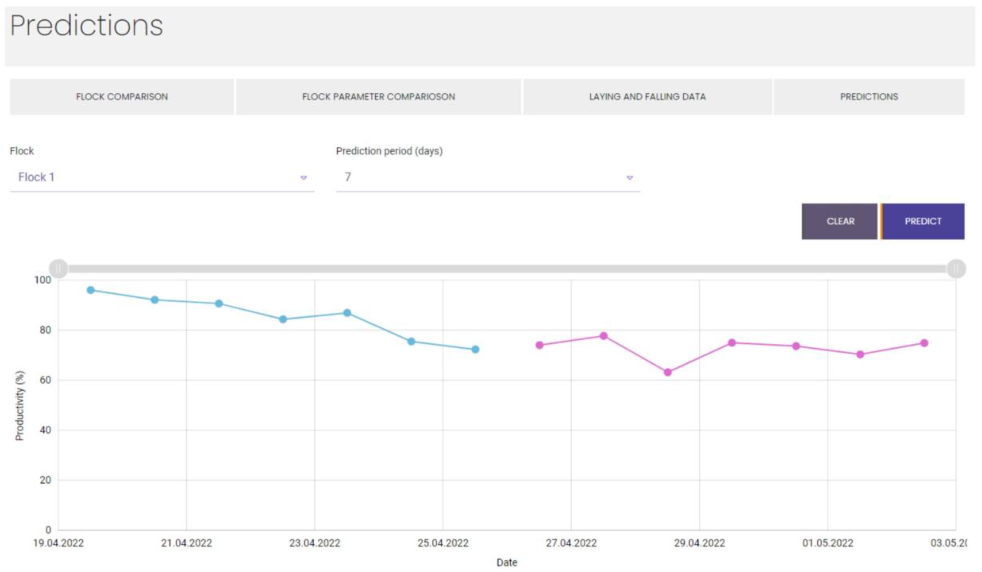
During the development stage, the developing models were implemented into the existing poultry management platform Aihen as a submodule for hen egg production forecasting [52]. Figure 7 depicts the example of an implementation when the data were actively gathered and analysed, including the testing phase of the model’s development.

4. Discussion

The egg production cycle used for model testing was atypical in terms of data quality characteristics—uniformity and completeness for instance—thus adding more complexity in the process of selecting the most viable model and forecasting egg production based on such data.

Regarding the importance of data quality, various measures can be taken. Applied techniques include outlier detection and removal and missing value generation (by interpolating neighbour values or association with another parameter). In general, data quality must take place as one of the steps of pre-processing: the distribution of data must be analysed, and either normalization or standardization might be applied; the data must be checked for noise (mostly sensor related data) and addressed accordingly. Therefore, additional duplicate sensors can be included in the farm. Unless the quality is at its lowest, the general techniques for improvement should be sufficient to reduce impact on ML prediction, and, whereas minor imperfections may affect ML parameters, the trendline of outcome should be roughly the same. All of this would require the re-training and re-testing of the model with different levels of data quality.

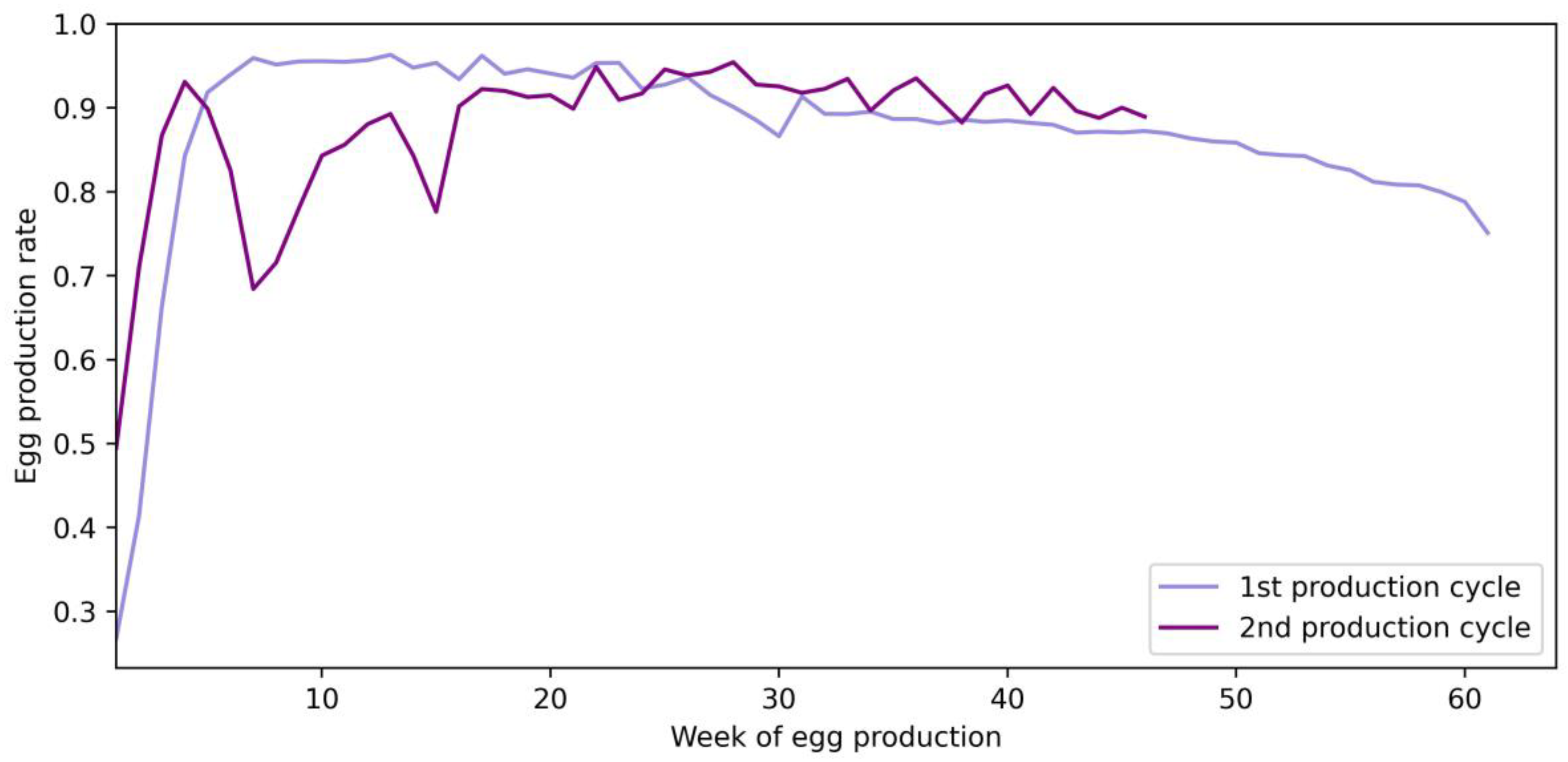
It must be noted that forecasting was performed for 1 day upfront only, which relatively limited the requirements for precision target. Additionally, while it was possible to forecast the production rate for longer periods, the results may have seen a rapid decrease in precision; thus, the appropriate forecasting length should be long enough to implement appropriate changes (i.e., adapt the ventilation algorithm for temperature changes) to the production process. In addition, the choice of forecasting only 1 day upfront was dictated by the consistency in the available training data. This also included differences between data of two separate cycles (as demonstrated in Figure 2).

Another aspect that should be researched more is the number of factors needed to provide a reliable prediction. This could be important for smaller farms that might not have multi-sensor equipment to measure various parameters that affect hen egg production (such as CO₂, NH₃). A study carried out by [42] was aimed to determine the environmental factors that influence the egg production of laying waterfowls’ (lion-head goose). The authors found that the optimal number of parameters was equal to four (i.e., laying rate, carbon dioxide, temperature, and dust) when forecasting, using a combination of LSTM and RF. While it may have some differences, the general guidelines of having limited parameters, which can be observed consistently, may be projected to laying hens as well, but further studies (larger datasets) and practical evidential assessments are still required to confirm this.

In the process of finding the optimal set of parameters, a lot of redundant and unimportant factors may be introduced that may lead the model astray; thus, we can assume that convoluting models with multiple parameters not only increase the difficulty for the data gathering step but may also lead to a decrease in the overall performance in regard to accurate forecasting.

5. Conclusions

The test data set that was significantly different demonstrated the limitations of the nonlinear model that used only one parameter (the number of weeks laying) and did not adjust to changes that also resulted in MAPE and RMSPE values—9.134% and 14.809%, respectively.

Although the calculated errors (MAPE and RMSPE) of the ML models were within the range of 5% to 10%, it was observed that they could better adjust to production changes than the tested nonlinear regression model.

As the ML models also used environmental data as inputs, sudden changes in those factors (e.g., temperature, CO₂, NH₃) affected productivity, which could be predicted in a timely manner.

The results showed that the ML models (LSTM, RF, and XGBoost, with a sliding window size of two) were able to forecast the drop-in production rate (2nd production cycle) at a satisfactory level.

The results suggested that the proposed solutions may also be applicable within farms that have limited production data sets and do not have large volumes of historical egg production data.

Depending on the available historical data for model training, the farm could also employ a multi-model approach, where different models could be run according to the farmer’s needs (forecasting length). Furthermore, this also keeps an option to apply the nonlinear model in situations where no environmental or other productivity-affecting data are recorded. In this case, the nonlinear model could be used either as a separate solution or complementary evidence to follow the production curve dynamics.

References

1. França, R.D.S.; Correa, F.; Maria, T.C.; Ribeiro, J.S.D.A.N.; Ferreira, E.D.P. Transformação Agrícola Digital: O Entrelaçamento da Agricultura E Transformação Digital Para O Futuro Inovador Do Setor Agrícola. Exacta 2021. [Google Scholar] [CrossRef]
2. Pitesky, M.; Gendreau, J.; Bond, T.; Carrasco-Medanic, R. Data challenges and practical aspects of machine learning-based statistical methods for the analyses of poultry data to improve food safety and production efficiency. CAB Rev. Perspect. Agric. Vet. Sci. Nutr. Nat. Resour. 2020, 15, 1–11. [Google Scholar] [CrossRef]
3. Wang, C.-Y.; Chen, Y.-J.; Chien, C.-F. Industry 3.5 to empower smart production for poultry farming and an empirical study for broiler live weight prediction. Comput. Ind. Eng. 2020, 151, 106931. [Google Scholar] [CrossRef]
4. Ahmad, H.A. Egg production forecasting: Determining efficient modeling approaches. J. Appl. Poult. Res. 2011, 20, 463–473. [Google Scholar] [CrossRef] [PubMed]
5. Astill, J.; Dara, R.A.; Fraser, E.D.; Roberts, B.; Sharif, S. Smart poultry management: Smart sensors, big data, and the internet of things. Comput. Electron. Agric. 2020, 170, 105291. [Google Scholar] [CrossRef]
6. Orakwue, S.I.; Al-Khafaji, H.M.R.; Chabuk, M.Z. IoT Based Smart Monitoring System for Efficient Poultry Farming. Webology 2022, 19, 4105–4112. [Google Scholar] [CrossRef]
7. Revanth, M.; Kumar, K.S.; Srinivasan, M.; Stonier, A.A.; Vanaja, D.S. Design and Development of an IoT Based Smart Poultry Farm. In Proceedings of the 2021 International Conference on Advancements in Electrical, Electronics, Communication, Computing and Automation (ICAECA), Coimbatore, India, 8–9 October 2021. [Google Scholar] [CrossRef]
8. European Union. Commission Directive 2000/39/EC of 8 June 2000 Establishing a First List of Indicative Occupational Exposure Limit Values in Implementation of Council Directive 98/24/EC on the Protection of the Health and Safety of Workers from the Risks Related to Chemical Agents at Work. Off. J. Eur. Communities 2000, L 142, 47. Available online: http://data.europa.eu/eli/dir/2000/39/2018-08-21 (accessed on 21 June 2022).
9. European Union. Council directive 1999/74/EC of 19 July 1999, laying down minimum standards for the protection of laying hens. Off. J. Eur. Communities 1999, L 203, 53–57. Available online: http://data.europa.eu/eli/dir/1999/74/oj (accessed on 21 June 2022).
10. European Union. Council Directive 2007/43/EC of 28 June 2007 laying down minimum rules for the protection of chickens kept for meat production. Off. J. Eur. Communities 2007, 19. Available online: http://data.europa.eu/eli/dir/2007/43/2019-12-14 (accessed on 21 June 2022).
11. Baku: Poultry IOT Solution. 2022. Available online: https://baku.global/en/smart-farming-poultry-iot-solution/ (accessed on 21 June 2022).
12. Fancom: Smart Farming. 2022. Available online: https://www.fancom.com/smart-farming (accessed on 21 June 2022).
13. Arhipova, I.; Vitols, G.; Paura, L.; Jankovska, L. Smart Platform Designed to Improve Poultry Productivity and Reduce Greenhouse Gas Emissions. In Lecture Notes in Networks and Systems; Springer Science and Business Media Deutschland GmbH: Berlin/Heidelberg, Germany, 2022; Volume 235, pp. 35–46. [Google Scholar]
14. Bumanis, N.; Arhipova, I.; Paura, L.; Vitols, G.; Jankovska, L. Data Conceptual Model for Smart Poultry Farm Management System. Procedia Comput. Sci. 2022, 200, 517–526. [Google Scholar] [CrossRef]
15. Paura, L.; Arhipova, I.; Jankovska, L.; Bumanis, N.; Vitols, G.; Adjutovs, M. Evaluation and association of laying hen performance, environmental conditions and gas concentrations in barn housing system. Ital. J. Anim. Sci. 2022, 21, 694–701. [Google Scholar]
16. Okinda, C.; Nyalala, I.; Korohou, T.; Okinda, C.; Wang, J.; Achieng, T.; Shen, M. A review on computer vision systems in monitoring of poultry: A welfare perspective. Artif. Intell. Agric. 2020, 4, 184–208. [Google Scholar]
17. Sakomura, N.K.; Reis, M.D.P.; Ferreira, N.T.; Gous, R.M. Modeling egg production as a means of optimizing dietary nutrient contents for laying hens. Anim. Front. 2019, 9, 45–51. [Google Scholar] [CrossRef]
18. Morales-Suárez, W.; Ospina-Rojas, I.C.; Méndez-Arteaga, J.J.; Ferreira, A.H.D.N.; Váquiro-Herrera, H.A. Multivariate modeling strategies to predict nutritional requirements of essential amino acids in semiheavy second-cycle hens. Rev. Bras. Zootec. 2021, 50, 1–20. [Google Scholar] [CrossRef]
19. Buller, H.; Blokhuis, H.; Lokhorst, K.; Silberberg, M.; Veissier, I. Animal Welfare Management in a Digital World. Animals 2020, 10, 1779. [Google Scholar] [CrossRef]
20. Murillo, A.C.; Abdoli, A.; Blatchford, R.A.; Keogh, E.J.; Gerry, A.C. Parasitic mites alter chicken behaviour and negatively impact animal welfare. Sci. Rep. 2020, 10, 8236. [Google Scholar] [CrossRef]
21. Görgülü, O.; Akilli, A. Egg production curve fitting using least square support vector machines and nonlinear regression analysis. Eur. Poult. Sci. 2018, 82, 1612–9199. [Google Scholar] [CrossRef]
22. Grossman, M.; Gossman, T.N.; Koops, W.J. A model for persistency of egg production. Poult. Sci. 2000, 79, 1715–1724. [Google Scholar] [CrossRef]
23. Safari-Aliqiarloo, A.; Faghih-Mohammadi, F.; Zare, M.; Seidavi, A.; Laudadio, V.; Selvaggi, M.; Tufarelli, V. Artificial neural network and non-linear logistic regression models to fit the egg production curve in commercial-type broiler breeders. Eur. Poult. Sci. 2017, 81. [Google Scholar] [CrossRef]
24. Felipe, V.P.S.; Silva, M.A.; Valente, B.D.; Rosa, G.J.M. Using multiple regression, Bayesian networks and artificial neural networks for prediction of total egg production in European quails based on earlier expressed phenotypes. Poult. Sci. 2015, 94, 772–780. [Google Scholar] [CrossRef]
25. Narinc, D.; Uckardes, F.; Aslan, E. Egg production curve analyses in poultry science. World’s Poult. Sci. J. 2014, 70, 817–828. [Google Scholar] [CrossRef]
26. Omomule, T.G.; Ajayi, O.O.; Orogun, A.O. Fuzzy prediction and pattern analysis of poultry egg production. Comput. Electron. Agric. 2020, 171, 105301. [Google Scholar] [CrossRef]
27. Wood, P.D.P. Algebraic Model of the Lactation Curve in Cattle. Nature 1967, 216, 164–165. [Google Scholar] [CrossRef]
28. McNally, D.H. 315. Note: Mathematical Model for Poultry Egg Production. Biometrics 1971, 27, 735. [Google Scholar] [CrossRef]
29. Adams, C.J.; Bell, D.D. Predicting Poultry Egg Production. Poult. Sci. 1980, 59, 937–938. [Google Scholar] [CrossRef]
30. McMillan, I. Compartmental Model Analysis of Poultry Egg Production Curves. Poult. Sci. 1981, 60, 1549–1551. [Google Scholar] [CrossRef]
31. Cason, J.A. Comparison of Linear and Curvilinear Decreasing Terms in Logistic Flock Egg Production Models. Poult. Sci. 1990, 69, 1467–1470. [Google Scholar] [CrossRef]
32. Yang, N.; Wu, C.; McMillan, I. New Mathematical Model of Poultry Egg Production. Poult. Sci. 1989, 68, 476–481. [Google Scholar] [CrossRef]
33. Faridi, A.; Mottaghitalab, M.; Rezaee, F.; France, J. Narushin-Takma models as flexible alternatives for describing economic traits in broiler breeder flocks. Poult. Sci. 2011, 90, 507–515. [Google Scholar] [CrossRef]
34. Savegnago, R.P.; Cruz, V.A.R.; Ramos, S.B.; Caetano, S.L.; Schmidt, G.S.; Ledur, M.C.; El Faro, L.; Munari, D.P. Egg production curve fitting using nonlinear models for selected and nonselected lines of White Leghorn hens. Poult. Sci. 2012, 91, 2977–2987. [Google Scholar] [CrossRef]
35. Nelder, J.A. The Fitting of a Generalization of the Logistic Curve. Biometrics 1961, 17, 89. [Google Scholar] [CrossRef]
36. Emam, A. Evaluation of Four Nonlinear Models Describing Egg Production Curve of Fayoumi Layers. Egypt. Poult. Sci. J. 2021, 41, 147–159. [Google Scholar] [CrossRef]
37. Sharifi, M.A.; Patil, C.S.; Yadav, A.S.; Bangar, Y.C. Mathematical modeling for egg production and egg weight curves in a synthetic white leghorn. Poult. Sci. 2022, 101, 101766. [Google Scholar] [CrossRef]
38. Li, D.; Tong, Q.; Shi, Z.; Zheng, W.; Wang, Y.; Li, B.; Yan, G. Effects of Cold Stress and Ammonia Concentration on Productive Performance and Egg Quality Traits of Laying Hens. Animals 2020, 10, 2252. [Google Scholar] [CrossRef]
39. Morales, I.R.; Cebrián, D.R.; Blanco, E.F.; Sierra, A.P. Early warning in egg production curves from commercial hens: A SVM approach. Comput. Electron. Agric. 2016, 121, 169–179. [Google Scholar] [CrossRef]
40. Ramírez-Morales, I.; Fernández-Blanco, E.; Rivero, D.; Pazos, A. Automated early detection of drops in commercial egg production using neural networks. Br. Poult. Sci. 2017, 58, 739–747. [Google Scholar] [CrossRef] [Green Version]
41. Shadrin, D.; Menshchikov, A.; Somov, A.; Bornemann, G.; Hauslage, J.; Fedorov, M. Enabling Precision Agriculture through Embedded Sensing with Artificial Intelligence. IEEE Trans. Instrum. Meas. 2019, 69, 4103–4113. [Google Scholar] [CrossRef]
42. Yin, H.; Liu, C.; Gao, Y.; Fan, W.; Xiao, B.; Cao, L.; Hassan, S.G.; Liu, S. A Novel Method to Predict Laying Rate Based on Multiple Environment Variables. IEEE Access 2021, 9, 115488–115496. [Google Scholar] [CrossRef]
43. Lubich, J.; Thomas, K.; Engels, D.W. Identification and Classification of Poultry Eggs: A Case Study Utilizing Computer Vision and Machine Learning. SMU Data Sci. Rev. 2019, 2, 24. [Google Scholar]
44. Maindonald, J.H. Data Mining with Rattle and R: The Art of Excavating Data for Knowledge Discovery by Graham Williams. Int. Stat. Rev. 2012, 80, 199–200. [Google Scholar] [CrossRef]
45. Chen, T.; Guestrin, C. XGBoost: A Scalable Tree Boosting System. In Proceedings of the KDD ’16: 22nd ACM SIGKDD International Conference on Knowledge Discovery and Data Mining, San Francisco, CA, USA, 13–17 August 2016; pp. 785–794. [Google Scholar] [CrossRef] [Green Version]
46. Chollet, F. Keras. GitHub. 2015. Available online: https://github.com/fchollet/keras (accessed on 18 May 2022).
47. Pedregosa, F.; Varoquaux, G.; Gramfort, A.; Michel, V.; Thirion, B.; Grisel, O.; Duchesnay, E. Scikit-learn: Machine Learning in Python. J. Mach. Learn. Res. 2011, 12, 2825–2830. [Google Scholar]
48. Bergstra, J.; Bengio, Y. Random search for hyper-parameter optimization. J. Mach. Learn. Res. 2012, 13, 281–305. [Google Scholar]
49. Hannun, A.; Guo, C.; van der Maaten, L. Measuring Data Leakage in Machine-Learning Models with Fisher Information. In Proceedings of the 37th Conference on Uncertainty in Artificial Intelligence, UAI 2021, Online, 27–30 July 2021; pp. 760–770. [Google Scholar]
50. Ying, X. An Overview of Overfitting and its Solutions. J. Phys. Conf. Ser. 2019, 1168, 022022. [Google Scholar] [CrossRef]
51. R Core Team. A Language and Environment for Statistical Computing. 2009. Available online: http://www.R-project.org (accessed on 11 March 2022).
52. Bumanis, N.; Kviesis, A.; Tjukova, A.; Arhipova, I.; Paura, L.; Vitols, G. Smart Poultry Management Platform with Egg Production Forecast Capabilities. Procedia Comput. Sci. 2023, 217, 339–347. [Google Scholar] [CrossRef]
Figure 1. The concept of a cyber–physical model (a) and the interrelationship of data in the proposed data structure (b) [14].
Applsci 13 07607 g001
Figure 2. Egg production curves used for training (1st cycle) and testing (2nd cycle).
Applsci 13 07607 g002
Figure 3. Environmental (temperature and relative humidity, represented by blue and orange colored lines, respectively) and feeding data (feed and water consumption per hen, represented by green and red colored lines, respectively) recorded during 1st (left side) and 2nd (right side) production cycle.
Applsci 13 07607 g003
Figure 4. Input and output parameters for ML models.
Applsci 13 07607 g004
Figure 5. Fitted curve and observed egg production rate.
Applsci 13 07607 g005
Figure 6. Results of the trained ML models tested on the 2nd production cycle.
Applsci 13 07607 g006
Figure 7. Example of prediction page. Blue curve represents actual data, pink—predicted [52].
Applsci 13 07607 g007