On Isospectral Composite Beams

Abstract

We consider a composite system consisting of two identical straight elastic beams under longitudinal vibration connected by an elastic interface capable of counteracting the relative vibration of the two beams with its shearing stiffness. We construct examples of isospectral composite beams, i.e., countable one-parameter families of beams having different shearing stiffness but exactly the same eigenvalues under a given set of boundary conditions. The construction is explicit and is based on the reduction to a one-dimensional Sturm–Liouville eigenvalue problem and the application of a Darboux’s lemma.

1. Introduction

Composite beams obtained by connecting two beam elements represent a structural solution commonly used in designing long-span floor beams or bridge decks [1]. The connection is the structural component having to bear the major consequences of stress and fatigue during service, and therefore, the evaluation of its integrity is of great importance for practical purposes. Nondestructive techniques based on dynamic measurements are appealing for assessing damage to composite beams and have attracted much interest in recent years; see, for example, [2,3] and the references therein.

In this paper, we consider a class of composite beams formed by two identical straight elastic beams connected together and subjected to longitudinal vibration. Practical examples of this system are steel beams connected by an adhesive layer on the contact surface and wood beams connected by means of wood studs that hinder sliding at the common interface. A schematic view can be seen in Figure 1. In mathematical terms, the small free undamped longitudinal vibration of such a composite beam of length L is governed by the differential system in $(z,t)\in (0,L)\times (0,T_0)$ [2]

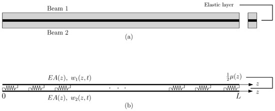
Figure 1. (a) Longitudinal view and cross-section of the composite beam. (b) Mechanical model for axial vibration.

$${\displaystyle \left\{\begin{array}{cc}\frac{\partial }{\partial z}\left(EA\left(z\right)\frac{\partial w_1}{\partial z}\right)+\frac{\mu \left(z\right)}{2}(w_2-w_1)=\gamma A\left(z\right)\frac{{\partial }^2{w}_1}{\partial t^2},\hfill & \hfill \mathrm{(1)}\\ \frac{\partial }{\partial z}\left(EA\left(z\right)\frac{\partial w_2}{\partial z}\right)-\frac{\mu \left(z\right)}{2}(w_2-w_1)=\gamma A\left(z\right)\frac{{\partial }^2{w}_2}{\partial t^2},\hfill & \hfill \mathrm{(2)}\end{array}\right.}$$

with supported end conditions at both ends, namely

$$w_1(0,t)=w_1(L,t)=0,w_2(0,t)=w_2(L,t)=0,t\in (0,T_0),$$

(3)

where $w_1(z,t)$, $w_2(z,t)$ is the axial displacement of the transversal section of beams 1 and 2, respectively, at the transversal section of abscissa z at the moment of time t, where $T_0>0$. The area of the cross-section is denoted by $A\left(z\right)$, $A\in C^2\left([0,L]\right)$, $A\left(z\right)\ge A_0>0$ in $[0,L]$. E is the Young’s modulus of the material, and $\gamma$ is the volume mass density. E and $\gamma$ are assumed to be constant and positive. The coefficient $\frac{\mu \left(z\right)}{2}$, $\mu \in C^0\left([0,L]\right)$, $\mu \left(z\right)\ge {\mu }_0>0$ in $[0,L]$ is the shearing stiffness per unit length of the connection.

For free vibration with a radian frequency $\omega$ and for a normalized abscissa $x=\frac{z}{L}$, the longitudinal displacement may be assumed as

$$w_1(x,t)=u_1\left(x\right)cos\left(\omega t\right),w_2(x,t)=u_2\left(x\right)cos\left(\omega t\right),$$

(4)

so that the eigenpair $\{\lambda ={\omega }^2\frac{\gamma L^2}{E},(u_1\left(x\right),u_2\left(x\right))\}$ satisfies

$${\displaystyle \left\{\begin{array}{cc}{\left(A{u}_1^{\prime }\right)}^{\prime }+\frac{k}{2}(u_2-u_1)+\lambda A{u}_1=0,x\in (0,1),\hfill & \hfill \mathrm{(5)}\\ {\left(A{u}_2^{\prime }\right)}^{\prime }-\frac{k}{2}(u_2-u_1)+\lambda A{u}_2=0,x\in (0,1),\hfill & \hfill \mathrm{(6)}\\ u_1\left(0\right)=u_1\left(1\right)=0,\hfill & \hfill \mathrm{(7)}\\ u_2\left(0\right)=u_2\left(1\right)=0,\hfill & \hfill \mathrm{(8)}\end{array}\right.}$$

where $k\left(x\right)=\frac{\mu \left(x\right)L^2}{E}$, $A\left(x\right)=A\left(\frac{z}{L}\right)$ and both $u_1\left(x\right)$ and $u_2\left(x\right)$ are not identically vanishing functions.

Assuming the beam profile $A\left(x\right)$ is given, an inverse problem that is interesting for applications consists of determining the shearing stiffness coefficient $k\left(x\right)$ from spectral data, e.g., the eigenvalues belonging to the spectrum under either Dirichlet or other boundary conditions. Putting

$$A=a^2,\mathbf{y}=(y_1=a{u}_1,y_2=a{u}_2),$$

(9)

system (5) and (6) reduces to the canonical Sturm–Liouville vectorial form

$${\mathbf{y}}^{″}+\lambda \mathbf{y}=\mathbf{Q}\mathbf{y},x\in (0,1),$$

(10)

with

$$\mathbf{Q}=\left(\begin{array}{cc}q+\frac{k}{2a^2}& -\frac{k}{2a^2}\\ -\frac{k}{2a^2}& q+\frac{k}{2a^2}\end{array}\right),$$

(11)

where the potential

$$q\left(x\right)=\frac{a^{″}\left(x\right)}{a\left(x\right)},q\in C^0\left([0,1]\right),$$

(12)

is given and $k\left(x\right)$ is the unknown coefficient.

Several results have been established for this class of inverse spectral problems, notably by Chern and Shen [4], Jodeit and Levitan [5,6], Shen [7], Getsezy and co-authors [8,9], Carlson [10], Andersson [11], Yurko [12], and Shieh [13], to mention a few. In particular, Shen [14] showed that a general two-by-two real symmetric smooth matrix $\mathbf{Q}$ can be uniquely determined by the eigenvalues belonging to five spectra corresponding to suitable boundary conditions. Chang and Shieh [15] extended the above result to the case of an integrable $m\times m$ general real matrix-valued symmetric function $\mathbf{Q}$, for which $1+m^2$ spectral data can determine $\mathbf{Q}$ uniquely.

By exploiting the special structure (11) of the matrix $\mathbf{Q}$ for our composite beam, we show here that the inverse problem of determining $k\left(x\right)$ in (10) and (11) can be framed within the one-dimensional Sturm–Liouville inverse spectral theory and that, roughly speaking, half of the eigenvalues of the Dirichlet spectrum in (5)–(8) and half of the eigenvalues of the cantilever spectrum (i.e., system (5) and (6) with $u_i\left(0\right)=u_i^{\prime }\left(1\right)=0$, $i=1,2$) of the composite beam uniquely determine the shearing stiffness $k\left(x\right)$. The analysis is based on the fact that this class of composite beams is spectrally equivalent to two families of one-dimensional Sturm–Liouville problems, and the eigenvalues of one family do not depend on the coefficient $k\left(x\right)$. We refer to Section 2 for a precise statement and related results.

Closely related to the inverse eigenvalue problem is the isospectrality problem for (5)–(8), i.e., the characterization of coefficients $k\left(x\right)$, which have the same spectrum as a given coefficient (with fixed $A\left(x\right)$) for a particular set of boundary conditions. In the scalar case, i.e., a single Sturm–Liouville equation in canonical form with scalar potential, the isospectrality problem was solved by Trubowitz and co-workers in [16,17,18,19]; see also the contributions by Coleman and McLaughlin for an impedance operator [20,21] and Gladwell and Morassi for applications to longitudinally vibrating beams [22] and for special classes of bending vibrating beams [23]. Jodeit and Levitan [5,6] proposed a method based on a Gelfand–Levitan integral equation and trasmutation operators for a general real symmetric matrix-valued smooth $m\times m$ matrix $\mathbf{Q}$, $m\ge 2$. Chelkak and Korotyaev [24] developed a method for a complete parametrization of the isospectral set of matrix-valued $L^1$-potentials. We refer also to Shieh [13] for uniqueness theorems for inverse problems for vectorial Sturm–Liouville equations in which all the eigenvalues of the system are of full multiplicity.

The above-mentioned papers deal with a complete characterization of the isospectral potentials $\mathbf{Q}$ for vector-valued Sturm–Liouville operators. As far as this aspect is concerned, the present paper has a more modest purpose: to show how to determine families of composite beams (with fixed $A\left(x\right)$) that are isospectral to a given one for a given set of boundary conditions. We will show that, under our assumptions, we can resort to a classical Darboux lemma [25] for an explicit construction of isospectral composite beams. The isospectral shearing stiffness coefficients $k\left(x\right)$ belong to a neighborhood of a given coefficient, and the construction is possible for composite beams with simple eigenvalues.

The paper is organized as follows. In Section 2, we show our main theoretical results concerning the unique determination of the shearing stiffness coefficient $k\left(x\right)$ from eigenvalue data and the construction of isospectral composite beams. Some examples are presented in Section 3. A generalization of the above analysis to composite systems formed by $N\ge 3$ connected beams is attempted in Section 4. We will see that the results are weaker in this case.

2. Theory

The following proposition establishes a spectral equivalence between the composite beam system (5)–(8) and two one-dimensional Sturm–Liouville problems.

Proposition 1.

Let $A\in C^2\left([0,1]\right)$, $A\left(x\right)\ge A_0$ in $[0,1]$, $k\in C^0\left([0,1]\right)$, and $k\left(x\right)\ge k_0$ in $[0,1]$, where $A_0$ and $k_0$ are positive constants.

Let $\{\lambda ,(u_1,u_2)\}$ be an eigenpair of the composite beam System (5)–(8). Then, either

$$u_2=u_1\mathrm{in}[0,1],$$

(13)

or, alternatively,

$$u_2=-u_1\mathrm{in}[0,1].$$

(14)

If (13) holds, then $\{{\lambda }^U,U=u_1+u_2\}$ is an eigenpair of

$${\displaystyle \left\{\begin{array}{cc}{\left(A{U}^{\prime }\right)}^{\prime }+{\lambda }^{U}AU=0,x\in (0,1),\hfill & \hfill \mathrm{(15)}\\ U\left(0\right)=U\left(1\right)=0.\hfill & \hfill \mathrm{(16)}\end{array}\right.}$$

If (14) holds, then $\{{\lambda }^V,V=u_1-u_2\}$ is an eigenpair of

$${\displaystyle \left\{\begin{array}{cc}{\left(A{V}^{\prime }\right)}^{\prime }+{\lambda }^{V}AV=kV,x\in (0,1),\hfill & \hfill \mathrm{(17)}\\ V\left(0\right)=V\left(1\right)=0.\hfill & \hfill \mathrm{(18)}\end{array}\right.}$$

Proof. 

The proof of (13) and (14) is by contradiction. Let us assume there exists a constant $\beta$ ($\beta \ne 0$) such that

$$u_2=\beta u_1\mathrm{in}[0,1],\left|\beta \right|\ne 1.$$

(19)

Using (19) in (5)–(8), we obtain

$$(\beta +1)({\left(A{u}_1^{\prime }\right)}^{\prime }+\lambda A{u}_1)=0\mathrm{in}(0,1)$$

(20)

which implies

$${\left(A{u}_1^{\prime }\right)}^{\prime }+\lambda A{u}_1=0\mathrm{in}(0,1).$$

(21)

Comparing (21) with (5), we conclude that

$$k(u_2-u_1)=0\mathrm{in}[0,1],$$

(22)

which implies $u_2=u_1$; that is, $\beta =1$, which is a contradiction.

Finally, the eigenvalue problems (15)–(16) and (17)–(18) follow from (5)–(8) by summing and subtracting (5) and (6), respectively, and by taking into account the boundary conditions. □

Remark 1.

Note that, in order to distinguish the two classes of principal modes, it is enough to know the axial strain $u_i^{\prime }$, where $i=1,2$, at one end of the beam, say $u_1^{\prime }\left(0\right)$, $u_2^{\prime }\left(0\right)$. In fact, for in-phase motion, we have $u_1^{\prime }\left(0\right)=u_2^{\prime }\left(0\right)$, whereas for out-of-phase vibration, we have $u_1^{\prime }\left(0\right)=-u_2^{\prime }\left(0\right)$. Note that $u_1^{\prime }\left(x\right)u_2^{\prime }\left(x\right)\ne 0$ for $x=0$ and $x=1$.

Remark 2.

The eigenvalues of (5)–(8) may not be simple, with multiplicity at most equal to 2. For the uniform composite beam with $A\left(x\right)=1$ and $k\left(x\right)=k_0$ constant, where $k_0>0$, the eigenvalues are double if and only if $k_0=(n^2-m^2){\pi }^2$ for integer numbers $m,n$ with $n>m\ge 1$. Clearly, if $0<k_0<3{\pi }^2$, then all the eigenvalues are simple.

Remark 3.

Proposition 1 can also be extended to other boundary conditions, for example, the cantilever end conditions:

$$u_1\left(0\right)=u_2\left(0\right)=0,u_1^{\prime }\left(1\right)=u_2^{\prime }\left(1\right)=0.$$

(23)

The eigenvalues ${\left\{{\lambda }_i^{\prime }\right\}}_{i\ge 1}$ of (5)–(6) and (23) are given by

$${\left\{{\lambda }_i^{\prime }\right\}}_{i\ge 1}={\left\{{\lambda }_l^{U^{\prime }}\right\}}_{l\ge 1}\cup {\left\{{\lambda }_n^{V^{\prime }}\right\}}_{n\ge 1},$$

(24)

where ${\left\{{\lambda }_l^{U^{\prime }}\right\}}_{l\ge 1}$, ${\left\{{\lambda }_n^{V^{\prime }}\right\}}_{n\ge 1}$ are, respectively, the eigenvalues of

$${\displaystyle \left\{\begin{array}{cc}{\left(A{U}^{\prime }\right)}^{\prime }+{\lambda }^{U^{\prime }}AU=0,x\in (0,1),\hfill & \hfill \mathrm{(25)}\\ U\left(0\right)=U^{\prime }\left(1\right)=0,\hfill & \hfill \mathrm{(26)}\end{array}\right.}$$

and

$${\displaystyle \left\{\begin{array}{cc}{\left(A{V}^{\prime }\right)}^{\prime }+{\lambda }^{V^{\prime }}AV=kV,x\in (0,1),\hfill & \hfill \mathrm{(27)}\\ V\left(0\right)=V^{\prime }\left(1\right)=0.\hfill & \hfill \mathrm{(28)}\end{array}\right.}$$

From Proposition 1, it is seen that, when the composite beam vibrates in the principal modes of (15) and (16), the two beams are subject to in-phase motions $(u_1,u_2=u_1)$, and the strain energy stored inside the connection vanishes. On the contrary, the two beams oscillate according to out-of-phase motions $(u_1,u_2=-u_1)$ when the composite beam vibrates in the principal modes of (17) and (18). These latter modes are the only principal modes affected by the shearing stiffness of the connection, and therefore, only the family of eigenvalues ${\left\{{\lambda }_n^V\right\}}_{n\ge 1}$ contains information about the stiffness of the connection. It follows that the problem of determining $k\left(x\right)$ from spectral data in (5)–(8) coincides with the problem of determining $k\left(x\right)$ in the scalar Sturm–Liouville Problem (17) and (18). By the Liouville transformation $(y=aV,A=a^2)$, Problems (17) and (18) can be reduced to the canonical form

$${\displaystyle \left\{\begin{array}{cc}{y}^{″}+\lambda y=\left(q+\frac{k}{a^2}\right)y,x\in (0,1),\hfill & \hfill \mathrm{(29)}\\ y\left(0\right)=y\left(1\right)=0,\hfill & \hfill \mathrm{(30)}\end{array}\right.}$$

with $q=\frac{a^{″}}{a}$. Inverse problems for (29) and (30) are well-known due to the cornerstone contributions by Borg [26], Levinson [27], Gelfand-Levitan [28], Hochstadt [29], and Hald [30], among others. For example, if $A\left(x\right)=A(1-x)$ (a given coefficient) and $k\left(x\right)=k(1-x)$ in $[0,1]$, then the Dirichlet spectrum ${\left\{{\lambda }_n^V\right\}}_{n\ge 1}$ uniquely determines the coefficient $k\left(x\right)$. The symmetry condition on $k\left(x\right)$ can be removed by adding a second spectrum corresponding, for example, to the set of eigenvalues ${\left\{{\lambda }_n^{V^{\prime }}\right\}}_{n\ge 1}$ of the cantilever end conditions. We refer to the above-mentioned papers and to the book by Gladwell [31] for more details on the uniqueness results and also on reconstruction strategies.

We now consider the determination of isospectral composite beams. Let ${\{\widehat{A}\left(x\right),\widehat{k}\left(x\right)\}}_2$ be a composite beam formed by two connected beams of cross-sectional area $A\left(x\right)$, and assume Dirichlet conditions at both ends. By Proposition 1, we know that ${\left\{{\lambda }_i\right\}}_{i\ge 1}={\left\{{\lambda }_l^U\right\}}_{l\ge 1}\cup {\left\{{\lambda }_n^V\right\}}_{n\ge 1}$, where ${\left\{{\lambda }_l^U\right\}}_{l\ge 1}$ does not depend on the shearing stiffness $k\left(x\right)$ and ${\left\{{\lambda }_n^V\left(\widehat{k}\left(x\right)\right)\right\}}_{n\ge 1}$ are the eigenvalues of

$${\displaystyle \left\{\begin{array}{cc}{\left(\widehat{A}{V}^{\prime }\right)}^{\prime }+{\lambda }^V\widehat{A}V=\widehat{k}V,x\in (0,1),\hfill & \hfill \mathrm{(31)}\\ V\left(0\right)=V\left(1\right)=0.\hfill & \hfill \mathrm{(32)}\end{array}\right.}$$

We wish to determine other shearing stiffness coefficients $k\left(x\right)$ such that all the eigenvalues of

$${\displaystyle \left\{\begin{array}{cc}{\left(\widehat{A}{V}^{\prime }\right)}^{\prime }+{\lambda }^V\widehat{A}V=kV,x\in (0,1),\hfill & \hfill \mathrm{(33)}\\ V\left(0\right)=V\left(1\right)=0,\hfill & \hfill \mathrm{(34)}\end{array}\right.}$$

coincide exaclty with the eigenvalues of (31) and (32), e.g.,

$${\lambda }_n^V\left(\widehat{k}\right)={\lambda }_n^V\left(k\right)\mathrm{for}\mathrm{every}n\ge 1.$$

(35)

As a first step, we reduce (31) to their canonical form via the Sturm–Liouville transformation $(y=\widehat{a}V,\widehat{A}={\widehat{a}}^2)$:

$${\displaystyle \left\{\begin{array}{cc}{y}^{″}+{\lambda }^{V}y=\left(\widehat{q}+\frac{\widehat{k}}{{\widehat{a}}^2}\right)y,x\in (0,1),\hfill & \hfill \mathrm{(36)}\\ y\left(0\right)=y\left(1\right)=0,\hfill & \hfill \mathrm{(37)}\end{array}\right.}$$

with $\widehat{q}=\frac{{\widehat{a}}^{″}}{\widehat{a}}$. Next, the analysis developed in [19] shows how to obtain a Sturm–Liouville operator with a potential q isospectral to the potential $\left(\widehat{q}+\frac{\widehat{k}}{{\widehat{a}}^2}\right)$. The analysis in [19] is based on a double application of a Darboux lemma [25]. For the sake of completeness, a brief description of the Darboux lemma is provided in Remark 5 below. It turns out that

$$q\left(x\right)=\widehat{q}\left(x\right)+\frac{\widehat{k}\left(x\right)}{{\widehat{a}}^2}-2\frac{d^2}{d{x}^2}\left(log\left(1+c{\int }_0^x{y}_m^2\left(s\right)ds\right)\right),$$

(38)

where $c>-1$ and $m=1,2,\dots$, and $y_m\left(x\right)$ is the mth Dirichlet eigenfunction of (36) and (37) normalized by ${\int }_0^1{y}_m^2\left(s\right)ds=1$. Therefore, assuming $q\left(x\right)=\widehat{q}\left(x\right)+\frac{k}{{\widehat{a}}^2}$, for every $m=1,2,\dots$, we obtain a composite beam ${\{\widehat{A}\left(x\right),k\left(x\right)\}}_2$ with shearing stiffness

$$k\left(x\right)=\widehat{k}\left(x\right)-2c{\widehat{a}}^2\left(x\right)y_m\left(x\right)\left(\frac{2y_m^{\prime }\left(x\right)}{1+c{\int }_0^x{y}_m^2\left(s\right)ds}-\frac{c{y}_m^3\left(x\right)}{{\left(1+c{\int }_0^x{y}_m^2\left(s\right)ds\right)}^2}\right),$$

(39)

which has exactly the same eigenvalues of ${\{\widehat{A}\left(x\right),\widehat{k}\left(x\right)\}}_2$, e.g., ${\lambda }_n^V\left(\widehat{k}\right)={\lambda }_n^V\left(k\right)$ for every $n\ge 1$. To conclude the construction of a real “physical” isospectral composite beam, we need to show that the shearing stiffness $k\left(x\right)$ is positive in $[0,1]$. Since, by hypothesis, $\widehat{k}\left(x\right)\ge k_0>0$ in $[0,1]$, by (39), there exists $k_0^{\prime }>0$, and there exists $\delta >0$ (possibly depending on m and $k_0^{\prime }$) such that $k\left(x\right)\ge k_0^{\prime }>0$ in $[0,1]$ for every $c>-1$ and $c\in [-\delta ,\delta ]$. In conclusion, the composite beam ${\{\widehat{A}\left(x\right),k\left(x\right)\}}_2$ is isospectral to ${\{\widehat{A}\left(x\right),\widehat{k}\left(x\right)\}}_2$ under Dirichlet end conditions.

Remark 4.

By adapting the above analysis and using the results in [22], it can be shown that the construction of isospectral composite beams also extends to other boundary conditions, such as, for example, the support–free (cantilever) and free–free conditions.

Remark 5.

Here, we recall the main steps for the determination of the potential $q\left(x\right)$ in (39) isospectral to the potential $(\widehat{q}+\widehat{k}/{\widehat{a}}^2)$ under Dirichlet boundary conditions. The analysis is based on a double application of the Darboux lemma [25]. Denote by $L_r$ the standard Sturm–Liouville operator with potential $r\in C\left(\right[0,1\left]\right)$, i.e., $L_{r}u=-u^{″}+ru$. Let μ, λ be two real numbers. In its simpler form, the Darboux lemma enables us to find a non-trivial solution z of a new equation $L_{\check{q}}z=\lambda z$ if we know a non-trivial solution g, f of the equation $L_{r}g=\mu g$, $L_{r}f=\lambda f$, respectively, corresponding to two different values λ, μ of the parameter and to a potential r. In particular, it turns out that $z=\frac{1}{g}[g,f]$, where $[g,f]=g{f}^{\prime }-g^{\prime }f$, and $\check{q}=r-2{(ln\left(g\right))}^{″}$. The potential $\check{q}$ is singular at those points of $[0,1]$ in which g has a zero. However, for such cases, we can modify the above analysis by applying the Darboux lemma twice, obtaining Expression (39) of the regular (i.e., continuous) potential q isospectral to $(\widehat{q}+\widehat{k}/{\widehat{a}}^2)$. We refer to the book [19] (Chapter 5) for more details.

3. Examples

As an application of the above results, we determine examples of composite beams that are isospectral to the uniform composite beam with $\widehat{A}\left(z\right)=1$, $\widehat{\mu }\left(z\right)={\pi }^2$, $E=1$, $\gamma =1$ and $L=1$ under supported-end conditions. A direct calculation shows that $\widehat{a}\left(x\right)=1$, $\widehat{k}\left(x\right)={\pi }^2$, $y_m\left(x\right)=\sqrt{2}sin\left(m\pi x\right)$, ${\widehat{\lambda }}_m^V=(1+m^2){\pi }^2$, $m=1,2,\dots$.

The isospectral composite beam has a shearing stiffness coefficient $k\left(x\right)$ given by (39). The isospectral coefficients shown in Figure 2 have been derived for $m=1$ and $c=-0.1,$ $c=-0.2$, and $c=-0.3$. The initial uniform beam corresponds to $c=0$. Similarly, isospectral coefficients for $m=2$, with $c=-0.05,c=-0.1,$ and $c=-0.2$ and for $m=5$ with $c=-0.08,c=-0.1,$ and $c=-0.12$ are shown in Figure 3 and Figure 4, respectively.

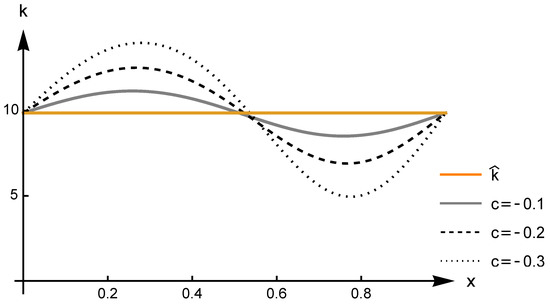
Figure 2. Isospectral stiffness coefficient $k\left(x\right)$ as in (39) for $m=1$ and $c=-0.1,-0.2,$ and $-0.3$.

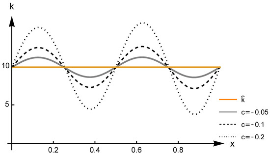
Figure 3. Isospectral stiffness coefficient $k\left(x\right)$ as in (39), for $m=2$ and $c=-0.05,-0.1,$ and $-0.2$.

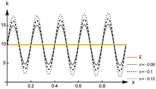
Figure 4. Isospectral stiffness coefficient $k\left(x\right)$ as in (39), for $m=5$ and $c=-0.08,-0.1,$ and $-0.12$.

It can be seen from these figures that when m is taken to be large, then the stiffness coefficient $k\left(x\right)$ depart significantly from that of the uniform beam $\widehat{k}\left(x\right)={\pi }^2$; that is, the change becomes more sensitive to changes in c.

The isospectral equivalence has been verified by finite element (FE) analysis. The numerical procedure herein adopted is based on a standard FE model of the problem (33) and (34) with a uniform mesh and continuous piecewise linear displacement shape functions ${\phi }_j={\phi }_j\left(x\right)$, where $j=1,2$. The local matrix entries of the stiffness $k_e^{ij}$ and mass matrix $m_e^{ij}$ are evaluated by the formulas

$$m_e^{ij}={\int }_{x_e}^{x_{e+1}}\widehat{A}{\phi }_i{\phi }_{j}dx,k_e^{ij}={\int }_{x_e}^{x_{e+1}}(\widehat{A}{\phi }_i^{\prime }{\phi }_j^{\prime }+k{\phi }_i{\phi }_j)dx,$$

(40)

where $i,j=1,2$, and are evaluated in exact form. A model with $N=200$ equally spaced finite elements was built by assembling the local matrices to form the global matrices and properly assigning the Dirichlet boundary conditions. For $N=200$, the first ten eigenvalues for the cases $c=-0.1$ and $m=5$ are given in Table 1 and are compared with the exact values corresponding to the uniform beam. It is seen that the constructed beams are isospectral to the original uniform beam within the limits of computing accuracy in such an FE approximation.

Table 1. Comparison between exact (${\lambda }_{exact}$) and FE results (${\lambda }_{FE}$) of the list ${\left({\lambda }_n\right)}_{n=1}^{10}$.

${\mathit{\lambda }}_{\mathit{e}\mathit{x}\mathit{a}\mathit{c}\mathit{t}}$ (rad/s)	19.74	49.35	98.70	167.78	256.61
${\lambda }_{FE}$	19.74	49.36	98.76	167.99	257.12
Error $\left(\frac{{\lambda }_{FE}-{\lambda }_{exact}}{{\lambda }_{exact}}\right)\times {10}^{-3}$	$0.13$	$0.32$	$0.67$	$1.24$	$1.98$
${\lambda }_{exact}$ (rad/s)	365.17	493.48	641.52	809.31	996.83
${\lambda }_{FE}$	366.23	495.43	644.86	814.65	1005.0
Error $\left(\frac{{\lambda }_{FE}-{\lambda }_{exact}}{{\lambda }_{exact}}\right)\times {10}^{-3}$	$2.89$	$3.96$	$5.20$	$6.60$	$8.17$

4. Extension to Multiple Connected Beams

Let us consider a supported composite system ${\{\widehat{A},\widehat{k}\}}_N$ obtained by connecting N equal beams, where $N\ge 2$, as considered in (5)–(8), with a cross-sectional area $\widehat{A}\left(x\right)$ and where the shearing stiffness of the $(N-1)$ connections is $\widehat{k}\left(x\right)$. The free axial vibration is governed by the boundary-value differential system

$${\displaystyle \left\{\begin{array}{cc}{\left(\widehat{A}{\mathbf{u}}^{\prime }\right)}^{\prime }+\lambda \widehat{A}\mathbf{u}={\displaystyle \frac{\widehat{k}\left(x\right)}{2}}\mathbf{C}\mathbf{u},x\in (0,1),\hfill & \hfill \mathrm{(41)}\\ \mathbf{u}\left(0\right)=\mathbf{u}\left(1\right)=0,\hfill & \hfill \mathrm{(42)}\end{array}\right.}$$

where $\mathbf{u}\left(x\right)=(u_1\left(x\right),\dots ,u_N\left(x\right))$ and where $\mathbf{C}$ is an $N\times N$ Jacobi matrix

$$\mathbf{C}=\left(\begin{array}{cccccc}1& -1& 0& \cdots & 0& 0\\ -1& 2& -1& \cdots & 0& 0\\ 0& -1& 2& \cdots & 0& 0\\ ⋮& ⋮& ⋮& \ddots & ⋮& ⋮\\ 0& 0& 0& \cdots & 2& -1\\ 0& 0& 0& \cdots & -1& 1\end{array}\right).$$

(43)

Let us represent $\mathbf{u}$ on the basis of the eigenvectors of $\mathbf{C}$, namely

$$\mathbf{u}\left(x\right)=\sum _{j=1}^N{\widehat{\eta }}^{\left(j\right)}\left(x\right){\mathbf{c}}^{\left(j\right)},{\widehat{\eta }}^{\left(j\right)}\left(x\right)=\mathbf{u}\left(x\right)·{\mathbf{c}}^{\left(j\right)},$$

(44)

where

$$\mathbf{C}{\mathbf{c}}^{\left(j\right)}={\chi }^{\left(j\right)}{\mathbf{c}}^{\left(j\right)},{\mathbf{c}}^{\left(j\right)}·{\mathbf{c}}^{\left(i\right)}={\delta }_{ij},$$

(45)

where $i,j=1,\dots ,N$. A direct calculation shows that, for every $j=1,\dots ,N$,

$${\displaystyle \left\{\begin{array}{cc}{\chi }^{\left(j\right)}=4{sin}^2\left({\displaystyle \frac{{\vartheta }_j}{2}}\right),\hfill & \hfill \mathrm{(46)}\\ {\vartheta }_j={\displaystyle \frac{(j-1)\pi }{N}},\hfill & \hfill \mathrm{(47)}\\ c_i^{\left(j\right)}={\displaystyle \frac{1}{{\overline{c}}_j}}cos\left({\displaystyle \frac{\vartheta }{2}}(2i-1)\right),i=1,\dots ,N,\hfill & \hfill \mathrm{(48)}\end{array}\right.}$$

where ${\overline{c}}_j$ are suitable positive normalization constants. Note that $0={\chi }^{\left(1\right)}<{\chi }^{\left(2\right)}<\cdots <{\chi }^{\left(N\right)}$. By using (44) in (41) and (42), and taking into account (45), we obtain the N uncoupled one-dimensional Sturm–Liouville eigenvalue problems for the functions ${\left\{{\widehat{\eta }}^{\left(i\right)}\left(x\right)\right\}}_{i=1}^N$:

$${\displaystyle \left\{\begin{array}{cc}{\left(\widehat{A}{\left({\widehat{\eta }}^{\left(i\right)}\right)}^{\prime }\right)}^{\prime }+\lambda \widehat{A}{\widehat{\eta }}^{\left(i\right)}={\chi }^{\left(i\right)}{\displaystyle \frac{\widehat{k}}{2}}{\widehat{\eta }}^{\left(i\right)},x\in (0,1),\hfill & \hfill \mathrm{(49)}\\ {\widehat{\eta }}^{\left(i\right)}\left(0\right)={\widehat{\eta }}^{\left(i\right)}\left(1\right)=0.\hfill & \hfill \mathrm{(50)}\end{array}\right.}$$

Note that in (49), the index i is fixed and not summed.

It follows that if $\lambda$ is an eigenvalue of the composite System (41) and (42), then $\lambda$ belongs to one family of the N Sturm–Liouville Problems (49) and (50) for some index i, $i=1,\dots ,N$, and vice versa.

We note that ${\chi }^{\left(1\right)}=0$ and ${\mathbf{c}}^{\left(1\right)}={\displaystyle \frac{1}{\sqrt{N}}}(1,\dots ,1)$; namely, the strain energy stored inside the $(N-1)$ connections of the composite system vanishes identically since the beams vibrate according to $\mathbf{u}\left(x\right)={\widehat{\eta }}^{\left(1\right)}\left(x\right){\mathbf{c}}^{\left(1\right)}$, which are all in phase with each other. The larger the index i, the larger the number of active connections, up to the case $i=N$, for which all beams vibrate out-of-phase to the adjacent ones.

We now attempt to generalise the procedure shown in Section 2 to the case $N\ge 3$. By the above analysis, the eigenvalues ${\left\{{\lambda }_k\right\}}_{k\ge 1}$ of ${\{\widehat{A},\widehat{k}\}}_N$ are given by

$${\left\{{\lambda }_k\right\}}_{k\ge 1}=\bigcup _{i=1}^N\bigcup _{n\ge 1}{\lambda }_n^{\left(i\right)},$$

(51)

where ${\left\{{\lambda }_n^{\left(i\right)}\right\}}_{n\ge 1}$ are the eigenvalues of (49) and (50).

Let us fix the index i, $i=2,\dots ,N$.

We first reduce (49), where $\lambda ={\lambda }^{\left(i\right)}$, to canonical form by defining $(y^{\left(i\right)}=\widehat{a}{\widehat{\eta }}^{\left(i\right)},\widehat{A}={\widehat{a}}^2)$ as

$${\displaystyle \left\{\begin{array}{cc}{\left(y^{\left(i\right)}\right)}^{″}+{\lambda }^{\left(i\right)}{y}^{\left(i\right)}=\left(\widehat{q}+\frac{{\chi }^{\left(i\right)}\widehat{k}}{{\widehat{a}}^2}\right)y^{\left(i\right)},x\in (0,1),\hfill & \hfill \mathrm{(52)}\\ y^{\left(i\right)}\left(0\right)=y^{\left(i\right)}\left(1\right)=0,\hfill & \hfill \mathrm{(53)}\end{array}\right.}$$

with $\widehat{q}={\displaystyle \frac{{\widehat{a}}^{″}}{\widehat{a}}}$. Next, we adapt the analysis based on Darboux’s lemma to obtain a new stiffness coefficient $k^{\left(i\right)}\left(x\right)$ isospectral to (49) and (50) (with $\lambda ={\lambda }^{\left(i\right)}$), namely,

$${\displaystyle \left\{\begin{array}{cc}{\left(\widehat{A}{\left({\eta }^{\left(i\right)}\right)}^{\prime }\right)}^{\prime }+{\lambda }^{\left(i\right)}\widehat{A}{\eta }^{\left(i\right)}={\chi }^{\left(i\right)}{\displaystyle \frac{k^{\left(i\right)}}{2}}{\eta }^{\left(i\right)},x\in (0,1),\hfill & \hfill \mathrm{(54)}\\ {\eta }^{\left(i\right)}\left(0\right)={\eta }^{\left(i\right)}\left(1\right)=0.\hfill & \hfill \mathrm{(55)}\end{array}\right.}$$

Here,

$${\chi }^{\left(i\right)}{k}^{\left(i\right)}\left(x\right)={\chi }^{\left(i\right)}\widehat{k}\left(x\right)-2c{\widehat{a}}^2\left(x\right)y_m^{\left(i\right)}\left(x\right)\left(\frac{2{\left(y_m^{\left(i\right)}\right)}^{\prime }\left(x\right)}{1+c{\int }_0^x{\left(y_m^{\left(i\right)}\right)}^{2}ds}-\frac{c{\left(y_m^{\left(i\right)}\right)}^3\left(x\right)}{{\left(1+c{\int }_0^x{\left(y_m^{\left(i\right)}\right)}^{2}ds\right)}^2}\right),$$

(56)

For a $c>-1$ and $\left|c\right|$ small enough, $m=1,2,\dots$, where $y_m^{\left(i\right)}\left(x\right)$ is the mth eigenfunction of (52) and (53). Note that $k^{\left(i\right)}$ also depends on the index i since $y_m^{\left(i\right)}$ depends on i.

We can now construct a composite system ${\{\widehat{A}\left(x\right),k^{\left(i\right)}\left(x\right)\}}_N$ such that all the eigenvalues ${\left\{{\lambda }_n^{\left(i\right)}\right\}}_{n\ge 1}$ of (54) and (55) belong to its spectrum. Let us multiply (54) by ${\mathbf{c}}^{\left(i\right)}$, where $\left(i\right)$ is a fixed index, not summed, where $i=2,\dots ,N$. Recalling (45), we have

$${\left(\widehat{A}{\left({\eta }_n^{\left(i\right)}\right)}^{\prime }{\mathbf{c}}^{\left(i\right)}\right)}^{\prime }+{\lambda }_n^{\left(i\right)}\widehat{A}{\eta }_n^{\left(i\right)}{\mathbf{c}}^{\left(i\right)}={\displaystyle \frac{k^{\left(i\right)}}{2}}\mathbf{C}\left({\eta }_n^{\left(i\right)}{\mathbf{c}}^{\left(i\right)}\right),x\in (0,1),$$

(57)

such that the function ${\mathbf{u}}_n^{\left(i\right)}={\eta }_n^{\left(i\right)}{\mathbf{c}}^{\left(i\right)}$ is a non-trivial solution to

$${\displaystyle \left\{\begin{array}{cc}{\left(\widehat{A}{\left({\mathbf{u}}_n^{\left(i\right)}\right)}^{\prime }\right)}^{\prime }+{\lambda }_n^{\left(i\right)}\widehat{A}{\mathbf{u}}_n^{\left(i\right)}={\displaystyle \frac{k^{\left(i\right)}\left(x\right)}{2}}\mathbf{C}{\mathbf{u}}_n^{\left(i\right)},x\in (0,1),\hfill & \hfill \mathrm{(58)}\\ {\mathbf{u}}_n^{\left(i\right)}\left(0\right)={\mathbf{u}}_n^{\left(i\right)}\left(1\right)=0.\hfill & \hfill \mathrm{(59)}\end{array}\right.}$$

We have proved that the composite systems ${\{\widehat{A},\widehat{k}\}}_N$, and ${\{\widehat{A},k^{\left(i\right)}\}}_N$ share the same eigenvalues ${\left\{{\lambda }_n^{\left(i\right)}\right\}}_{n\ge 1}$. However, if an index $j\ge 2$ is chosen with $j\ne i$, then $k^{\left(i\right)}$ and $k^{\left(j\right)}$ are not necessarily equal in $[0,1]$. It follows that, in general, it is not possible by this approach to construct isospectral composite systems unless, of course, $N=2$. This case was considered in Section 2.

5. Conclusions

In this paper, we have considered a special composite system formed by two equal elastic beams under axial vibration connected by an elastic interface with shearing stiffness k. We have shown how to construct composite systems with different shearing stiffness coefficients but with exactly all the same eigenvalues of an assigned system.

The analysis was based on reducing the free vibration problem of the composite system to two equivalent one-dimensional eigenvalue problems. The eigenvalues of one problem corresponded to in-phase motions of the two connected beams and did not depend on k. The other problem involved out-of-phase motions of the beams, and the eigenvalues depended on k. The application of a classical Darboux lemma to this second eigenvalue problem allowed the determination of explicit expressions of countable families of isospectral shearing stiffnesses, valid for various boundary conditions and in a sufficiently small neighbourhood of the initial stiffness. The extension of the above results to a composite system obtained by connecting $N\ge 3$ beams is, in general, not possible, at least by this approach, as discussed in Section 4.

The closed-form expressions of the isospectral shearing stiffness coefficients found in this paper are new in the literature of two-dimensional vector-valued Sturm–Liouville problems. Concerning possible engineering applications, our results confirm that the diagnostic problem of identifying the connection stiffness from natural frequency measurements only is severely ill-posed because the solution is clearly not unique. Secondly, the explicit expressions of the isospectral coefficients can be useful as a benchmark for estimating the accuracy of numerical models. Finally, our results may be used for designing the connection of a composite beam with assigned natural frequencies. This topic is the subject of ongoing research.

References

- Johnson, R.P. Composite Structures of Steel and Concrete, 1st ed.; Wiley Blackwell Scientific: New York, NY, USA, 2000. [Google Scholar]
- Morassi, A.; Nakamura, G.; Sini, M. An inverse dynamical problem for connected beams. Eur. J. Appl. Math. 2005, 16, 83–109. [Google Scholar] [CrossRef]
- Dilena, M.; Morassi, A. Vibrations of steel–concrete composite beams with partially degraded connection and applications to damage detection. J. Sound Vib. 2009, 320, 101–124. [Google Scholar] [CrossRef]
- Chern, H.-H.; Shen, C.-L. On the n-dimensional Ambarzumyan’s theorem. Inverse Probl. 1997, 13, 15–18. [Google Scholar] [CrossRef]
- Jodeit, M.; Levitan, B.M. The isospectrality problem for the classical Sturm-Liouville equation. Adv. Differ. Equ. 1997, 2, 297–318. [Google Scholar]
- Jodeit, M.; Levitan, B.M. Isospectral vector-valued Sturm-Liouville problems. Lett. Math. Phys. 1998, 43, 117–122. [Google Scholar] [CrossRef]
- Shen, C.-L. Some eigenvalue problems for the vectorial Hill’s equation. Inverse Probl. 2000, 16, 749–783. [Google Scholar] [CrossRef]
- Clark, S.; Gesztesy, F.; Holden, H.; Levitan, B.M. Borg-type theorems for matrix-valued Schrödinger operators. J. Differ. Equ. 2000, 167, 181–210. [Google Scholar] [CrossRef]
- Gesztesy, F.; Kiselev, A.; Levitan, B.M. Uniqueness results for matrix-valued Schrödinger, Jacobi and Dirac-type operators. Math. Nach. 2002, 239–240, 103–145. [Google Scholar] [CrossRef]
- Carlson, R. An inverse problem for the matrix Schrödinger equation. J. Math. Anal. Appl. 2002, 267, 564–575. [Google Scholar] [CrossRef][Green Version]
- Andersson, E. On the M-function and Borg-Marchenko theorems for vector-valued Sturm-Liouville equations. J. Math. Phys. 2003, 44, 6077–6100. [Google Scholar] [CrossRef]
- Yurko, V. Inverse problems for the matrix Sturm-Liouville equation on a finite interval. Inverse Probl. 2006, 22, 1139–1149. [Google Scholar] [CrossRef]
- Shieh, C.-T. Isospectral sets and inverse problems for vector-valued Sturm-Liouville equations. Inverse Probl. 2007, 23, 2457–2468. [Google Scholar] [CrossRef]
- Shen, C.-L. Some inverse spectral problems for vectorial Sturm-Liouville equations. Inverse Probl. 2001, 17, 1253–1294. [Google Scholar] [CrossRef]
- Chang, T.-H.; Shieh, C.-T. Uniqueness of the potential function for the vectorial Sturm-Liouville equation on a finite interval. Bound. Value Probl. 2011, 40. [Google Scholar] [CrossRef]
- Isaacson, E.L.; Trubowitz, E. The inverse Sturm-Liouville problem. I. Commun. Pure Appl. Math. 1983, 36, 767–783. [Google Scholar] [CrossRef]
- Isaacson, E.L.; McKean, H.P.; Trubowitz, E. The inverse Sturm-Liouville problem. II. Commun. Pure Appl. Math. 1984, 37, 1–11. [Google Scholar] [CrossRef]
- Dahlberg, B.E.J.; Trubowitz, E. The inverse Sturm-Liouville problem. III. Commun. Pure Appl. Math. 1984, 37, 255–267. [Google Scholar] [CrossRef]
- Pöschel, J.; Trubowitz, E. Inverse Spectral Theory, 1st ed.; Academic Press: London, UK, 1987. [Google Scholar]
- Coleman, C.F.; McLaughlin, J.R. Solution of the inverse spectral problem for an impedance with integrable derivative. I. Commun. Pure Appl. Math. 1993, 46, 145–184. [Google Scholar] [CrossRef]
- Coleman, C.F.; McLaughlin, J.R. Solution of the inverse spectral problem for an impedance with integrable derivative. II. Commun. Pure Appl. Math. 1993, 46, 185–212. [Google Scholar] [CrossRef]
- Gladwell, G.M.L.; Morassi, A. On isospectral rods, horns and strings. Inverse Probl. 1995, 11, 533–554. [Google Scholar] [CrossRef]
- Gladwell, G.M.L.; Morassi, A. A family of isospectral Euler-Bernoulli beams. Inverse Probl. 2010, 26, 035006. [Google Scholar] [CrossRef]
- Chelkak, D.; Korotyaev, E. Parametrization of the isospectral set for the vector-valued Sturm-Liouville problem. J. Funct. Anal. 2006, 241, 359–373. [Google Scholar] [CrossRef]
- Darboux, G. Sur la répresentation sphérique des surfaces. C. R. Math. Acad. Sci. Paris 1882, 1343–1345. [Google Scholar] [CrossRef]
- Borg, G. Eine Umkehrung der Sturm-Liouvilleschen Eigenwertaufgabe. Bestimmung der Differentialgleichung durch die Eigenwerte. Acta Math. 1946, 78, 1–96. [Google Scholar] [CrossRef]
- Levinson, N. The Inverse Sturm-Liouville Problem. Math. Tidsskr. B. 1949, 25–30. [Google Scholar]
- Gel’fand, I.M.; Levitan, B.M. On the determination of a differential equation from its spectral function. Am. Math. Soc. Transl. 1955, 2, 253–304. see also Izv. Math. Nauk SSSR 1951, 15, 309–360(In Russian) [Google Scholar]
- Hochstadt, H. The inverse Sturm–Liouville problem. Commun. Pure Appl. Math. 1973, 36, 715–729. [Google Scholar] [CrossRef]
- Hald, O.H. The inverse Sturm–Liouville problem with symmetric potentials. Acta Math. 1978, 141, 263–291. [Google Scholar] [CrossRef]
- Gladwell, G.M.L. Inverse Problems in Vibration, 2nd ed.; Kluwer Academic Publishers: Dordrecht, The Netherlands, 2004. [Google Scholar]
Disclaimer/Publisher’s Note: The statements, opinions and data contained in all publications are solely those of the individual author(s) and contributor(s) and not of MDPI and/or the editor(s). MDPI and/or the editor(s) disclaim responsibility for any injury to people or property resulting from any ideas, methods, instructions or products referred to in the content. |
© 2023 by the authors. Licensee MDPI, Basel, Switzerland. This article is an open access article distributed under the terms and conditions of the Creative Commons Attribution (CC BY) license (https://creativecommons.org/licenses/by/4.0/).