Constructing of 3D Fluvial Reservoir Model Based on 2D Training Images

Abstract

Training images are important input parameters for multipoint geostatistical modeling, and training images that can portray 3D spatial correlations are required to construct 3D models. The 3D training images are usually obtained by unconditional simulation using algorithms such as object-based algorithms, and in some cases, it is difficult to obtain the 3D training images directly, so a series of modeling methods based on 2D training images for constructing 3D models has been formed. In this paper, a new modeling method is proposed by synthesizing the advantages of the previous methods. Taking the fluvial reservoir modeling of the P oilfield in the Bohai area as an example, a comparative study based on 2D and 3D training images was carried out. By comparing the variance function, horizontal and vertical connectivity in x-, y-, and z-directions, and style similarity, the study shows that based on several mutually perpendicular 2D training images, the modeling method proposed in this paper can achieve an effect similar to that based on 3D training images directly. In the case that it is difficult to obtain 3D training images, the modeling method proposed in this paper has suitable application prospects.

1. Introduction

Multipoint geostatistics is the application of training images instead of variational functions to characterize the spatial relationships and distribution patterns between multiple points. After years of refinement and development, it has formed two types of multipoint geostatistics methods based on iterative and non-iterative algorithms. An important core of multipoint statistical 3D simulation lies in how to obtain training images. In order to obtain reasonable training images, scholars have proposed different methods, such as target-based simulation, 3D seismic information extraction or transformation, prototype-based model, depositional process-based method, and 2D images. Objective-based river simulation is temporarily inadequate in dealing with conditional simulation, mainly for the constraint of unconditional simulation without conditional data. It can produce well-formed river channels and natural levees, but the broken fan cannot be well characterized. For three-dimensional seismic information extraction or transformation, prototype model-based and depositional process-based methods are deterministic models. When the existing data are not perfect, there are always some uncertain factors in people’s understanding of it. It is difficult to grasp the real characteristics or properties of reservoirs at any scale, so if the reservoir has randomness, then these deterministic modeling methods will not be applicable. The biggest advantage of the two-dimensional image method is that it does not need three-dimensional training images and only needs a certain number of two-dimensional maps to realize multipoint geostatistical modeling. However, this method is difficult to quantitatively show the three-dimensional geometric characteristics and phase transition law of the reservoir, and its practicability is poor. The training image can be two-dimensional or three-dimensional, and the three-dimensional training image can be constructed by several methods. The first method is to build 3D training images directly using target-based or process-based algorithms; another method is to estimate the spatial distribution of the entire 3D model using statistical information obtained from multiple 2D training images [1,2,3,4,5,6]. However, in practical 3D applications, it is difficult to obtain 3D training images of some complex geological objects, such as the fallen silt layer inside the bar.

Hidajat et al. [7] constructed a 3D model using 2D images using the linear combination method mixed with the simulated annealing method, and the reconstructed tectonic model qualitatively matched with the original one, but the resolution of the training image needs to be improved. Youngseuk Keehm [8] and Zhu Yihua [9] both successfully reconstructed the real 3D pore medium model using 2D images using the sequential indication simulation method, and compared with other stochastic reconstruction methods (e.g., simulated annealing method), this method can better reproduce the connectivity, and the obtained 3D pore medium model is closer to the real rock structure, reflecting some real information of the formation. Liu Xuefeng et al. [10] reconstructed 3D mathematical cores based on 2D images of rocks and found that the 3D digital cores reconstructed by the process method have similar pore connectivity to the real cores, but only for sandstones. The pore connectivity of 3D digital cores constructed by the stochastic method represented by multipoint geostatistics and sequential indication simulation is poor. Wang Zhibao [11] used modern sedimentary data and dense well network channel spreading pattern data to build quantitative sedimentary microphase training images through field outcrops. By comparing the profiles, the established training images better reflect the quantitative distribution of each microphase. Bao Hongshuai [12] used two-dimensional images to quickly calculate the relationship between conductivity and porosity to determine the relationship between conductivity and porosity in three-dimensional digital cores. Compared with 3D microstructure, 2D microstructure information about rocks is more readily available and more common. However, many scholars have proposed methods to construct 3D models based on 2D training images to construct 3D digital cores by reconstruction methods (e.g., stochastic, process-based, and simulated annealing methods) based on the 2D microstructure information of rocks, all of which are unconditionally simulated [10,13,14]. However, in many cases, reservoir modeling directions are difficult to apply these methods, target-based or process-based, to construct 3D training images. For example, it is difficult to reproduce all types of geologic body geometries that can be represented by high-resolution outcrop mapping or considered non-smooth using the objective-based method.

Therefore, on the basis of previous studies, combining the advantages and disadvantages of the s2Dcd and DS methods, this paper proposes a new method to construct a three-dimensional fluvial reservoir model based on two-dimensional training images. The new algorithm combines the s2Dcd algorithm and the DS algorithm. Taking the modeling of the fluvial facies reservoir in the P oilfield in Bohai Bay as an example, the conditional simulation was carried out and compared with the Snesim and DS methods in terms of variation function, connectivity, and similarity. The algorithm uses multiple directional slices to reproduce the geometric features of fluvial geological space under reasonable constraints.

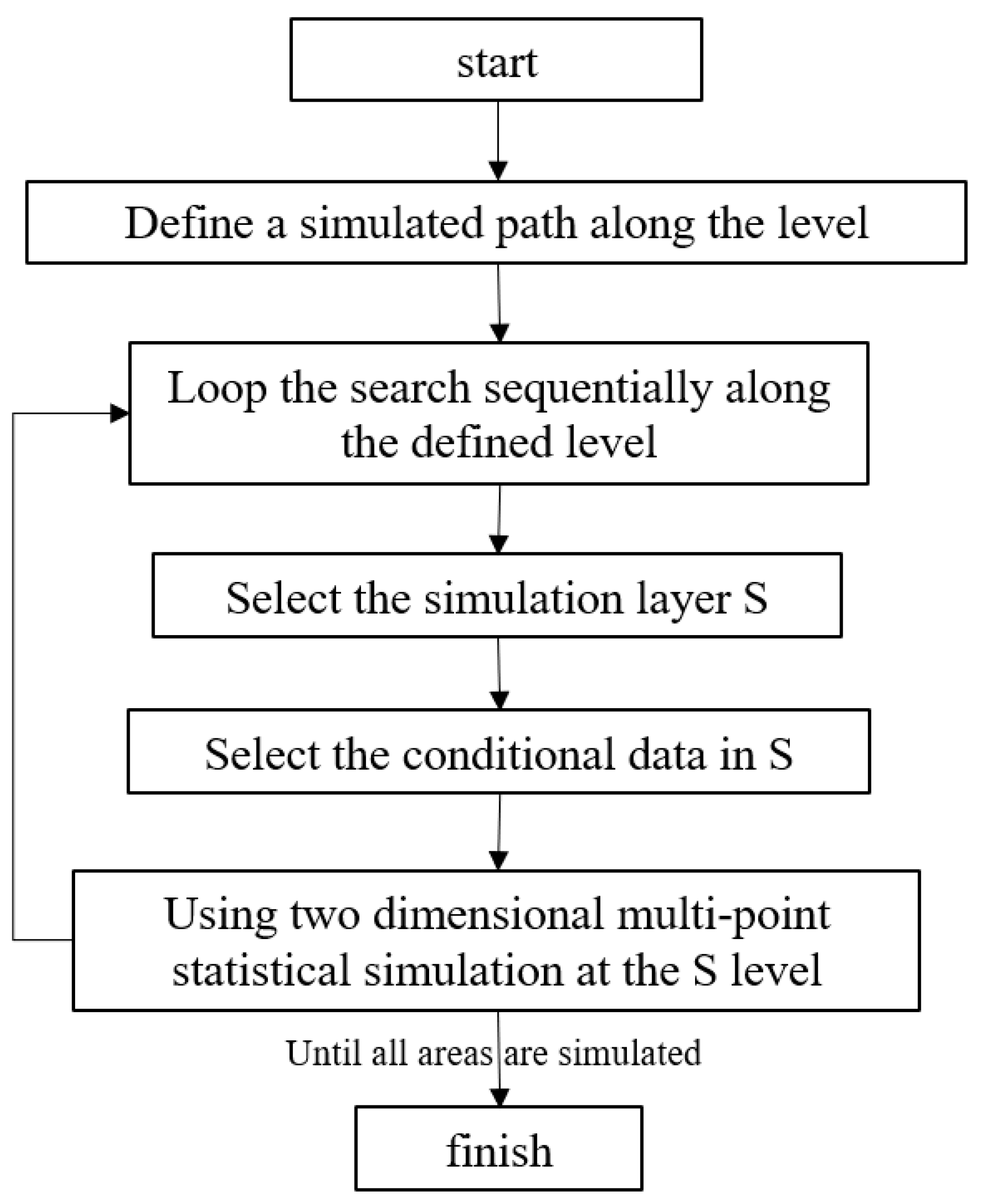
Introduction to the s2Dcd+DS Algorithm

In order to overcome the difficulties in acquiring 3D training images, Comunian et al. [15] proposed a sequential simulation method based on two-dimensional slices (s2Dcd for short) in 2012, with the flow chart shown in Figure 1. The key to this method is to define the sequence of the interfaces of the simulated layers and to include as many condition data points as possible. Sequential 2D conditional simulation is suitable when the condition data are sparse, and when the condition data are dense, the simulation quality slowly decreases due to the constraint of too much condition data. Comunian also suggests that different techniques can be mixed and a layered approach can be used, but the simulation framework may become complex, and its complexity mainly comes from the simulation of observations and taking into account non-smoothness.

The DS (direct sampling) algorithm is a multipoint modeling method based on the style proposed by Mariethoz in 2010, that is, assign values in the simulated grid according to the information of conditional points around each grid point until all points have values. The advantages of this method are: (1) it uses multipoint statistics information, so the whole pattern can be propagated; (2) because the neighborhood is flexible, it is possible to use patterns composed of irregular location data; (3) it can accommodate both categorical variables and continuous variables; (4) there is no problem with data relocation because there is no need for multiple grids. The disadvantage is that the simulation effect is poor when the conditional data are small [16,17].

The s2Dcd+DS algorithm combines the advantages of sequential two-dimensional conditional simulation and direct sampling simulation, weakens the influence of conditional data, reduces the simulation error, and achieves the ideal effect. Through algorithm fusion, multiple directional slices are used, and the advantages of the two methods are taken into account in the transverse and longitudinal morphological characteristics of the fluvial facies so as to ensure that the fluvial geological spatial geometric characteristics can be reproduced under reasonable constraints. The pseudo-code of the s2Dcd+DS algorithm is shown below, Algorithm 1.

Algorithm 1. s2Dcd+DS Algorithm Step
1.  INPUT TIs, condition datas(cds)
2.  INPUT analog mesh SG to achieve size
3.  DEFINE $\mathrm{RandomPath}$,radius_search,threads, Maxscan_Franction
4.	IMPORT the conditional data into SG according to the size of the simulated grid and the coordinates of each conditional data in the cds
5.  DEFINE setp_max
6.  WHILE true
7.  IF path_SG all simulation sequences have been accessed
8.  break WHILE LOOP
9.  END IF
10.     Create s2Dcd 2D simulation sequence
11.   x ← path SG’s next simulation sequence
12.   IF x is within the range defined setp_max
13.  IF The x simulation sequence contains cds, which is used as a constraint
14.        do Direct Sampling multipoint simulation
15.      ELSE
16.	The intersection location data of the previous simulated sequence is taken as the cds
17.        do Direct Sampling multipoint simulation
18.   END IF
19. OUTPUT model
20. END DO

The method simplifies the modeling process to a series of two-dimensional multipoint simulations by defining a two-dimensional simulation surface sequence. The operation steps of this method are as follows: (1) select the required two-dimensional training image, corresponding to step 10 of the pseudo-code; (2) define the two-dimensional random simulation surface sequence, and simulate the slices that pass through the most conditional data first, corresponding to step 13 of the pseudo-code; (3) perform DS simulation along the defined s2Dcd two-dimensional sequence, corresponding to step 14 of the pseudo-code; (4) until all grid nodes are simulated, corresponding to step 19 of the pseudo-code.

2. Three-Dimensional Condition Simulation of Fluvial Facies Reservoir

Taking the fluvial reservoir of the P oilfield in Bohai Bay as an example, this working area is located in the south of Bohai Bay, about 216.0 km away from Tanggu of Tianjin and about 80.0 km away from Penglai City of Shandong, as shown in Figure 2. The formation is located in Neogene Minghuazhen Formation, with 12 wells in the working area.

According to the types and distribution characteristics of sedimentary microfacies in the study area in

Table 1. Sedimentary facies characteristics of the study area.

Sedimentary Facies			Rock Type	Color	Sedimentary Structure	Structural Feature
Facies	Subphase	Microphase
Meander river	Meander channel	Edge beach	Gravelly medium sandstone, fine sandstone, and siltstone interbedded	Burgundy, brownish red, taupe	Trough cross-bedding, oblique bedding	Sorting medium, subridged, subrounded
		Channel retention
	Food plain	Flood plain	Mudstone, siltstone	Brownish red	Minor oblique bedding	Mainly argillaceous

, a three-dimensional training image of the work area was established. In order to simplify the simulation process, rock facies except sand were divided into the mud for simulation. Based on the 3D training image of the reservoir in the working area, the well data are imported, and the 3D model is established using the method proposed in this paper based on three mutually perpendicular 2D training images. At the same time, in order to compare with other methods, Snesim [18], a relatively mature multipoint geostatistical modeling method, will be used to build a three-dimensional model with three-dimensional training images, and the DS method will be used to build a three-dimensional model with two-dimensional training images. Comparative analysis will be conducted from three aspects, namely, variation function, sand body connectivity, and style similarity.

The specific operation steps of the Snesim algorithm are as follows: (1) Input the training image and the point to be estimated and select the appropriate data template. (2) Scan the training image with the data template. Data events that meet the data template are classified and stored to build a search tree. (3) Conditional data with known attributes are assigned to the nearest area to be estimated. (4) A random simulation path is defined. (5) Data events with the same geometric configuration as the estimated point are found in the search tree. The properties of the points to be estimated are randomly determined from the conditional probability distribution function (6), and the points to be estimated are added to the subsequent simulation as conditional data (7) to simulate the next point to be estimated along the simulation path. Repeat (4), (5), and (6) until all the attributes of the points to be estimated are obtained.

Using the target-based algorithm, parameters such as model mesh size, phase type, channel wavelength amplitude, and width were set, and a fluvial facies model with a mesh size of 100 × 100 × 50 was generated as a 3D training image (Figure 3a). Slices along x, y, and z in three different directions are obtained from the 3D model of the work area as 2D training images, as shown in Figure 3. The slice mesh sizes in the x-, y-, and z-directions were 100 × 100, 100 × 50, and 100 × 50, respectively (Figure 3b–d). The gray value is 0, indicating the background mud; a yellow value of 1 indicates channel sand. The well data distribution is shown in Figure 4.

Using 2D channel training images in three directions in Figure 3b–d and the conditional data obtained in Figure 4, the maximum scanning score was set at 0.3, and the grid size of the output model was 100 × 100 × 30 to generate three-dimensional models, grid models, and hollowed-out models, as shown in Figure 5. As can be seen from the grid diagram and hollow diagram of the model, the geometric morphology and spatial structure of the reconstructed model are better, and the visual results show that the three-dimensional model can be generated in accordance with the geological understanding by using two-dimensional slices.

The Snesim method uses a 3D training image in Figure 3a to generate a 3D geological model, and the DS method uses b-d three 2D training images in Figure 3 to simulate a 3D geological model. See Figure 6 for the 3D model generated by conditional simulation. The size of all models is set to 100 × 100 × 30. The geometric form of the 3D model reconstructed by the Snesim method is consistent with the geological cognition, while the 3D model reconstructed by the DS method has more noise and poor morphological performance.

3. Comparative Analysis

To test the effectiveness of the new method in reproducing the two-dimensional training image from the construction, the method in this paper is compared with the Snesim and DS methods from the variance function [19,20], comparative analysis of connectivity and style similarity.

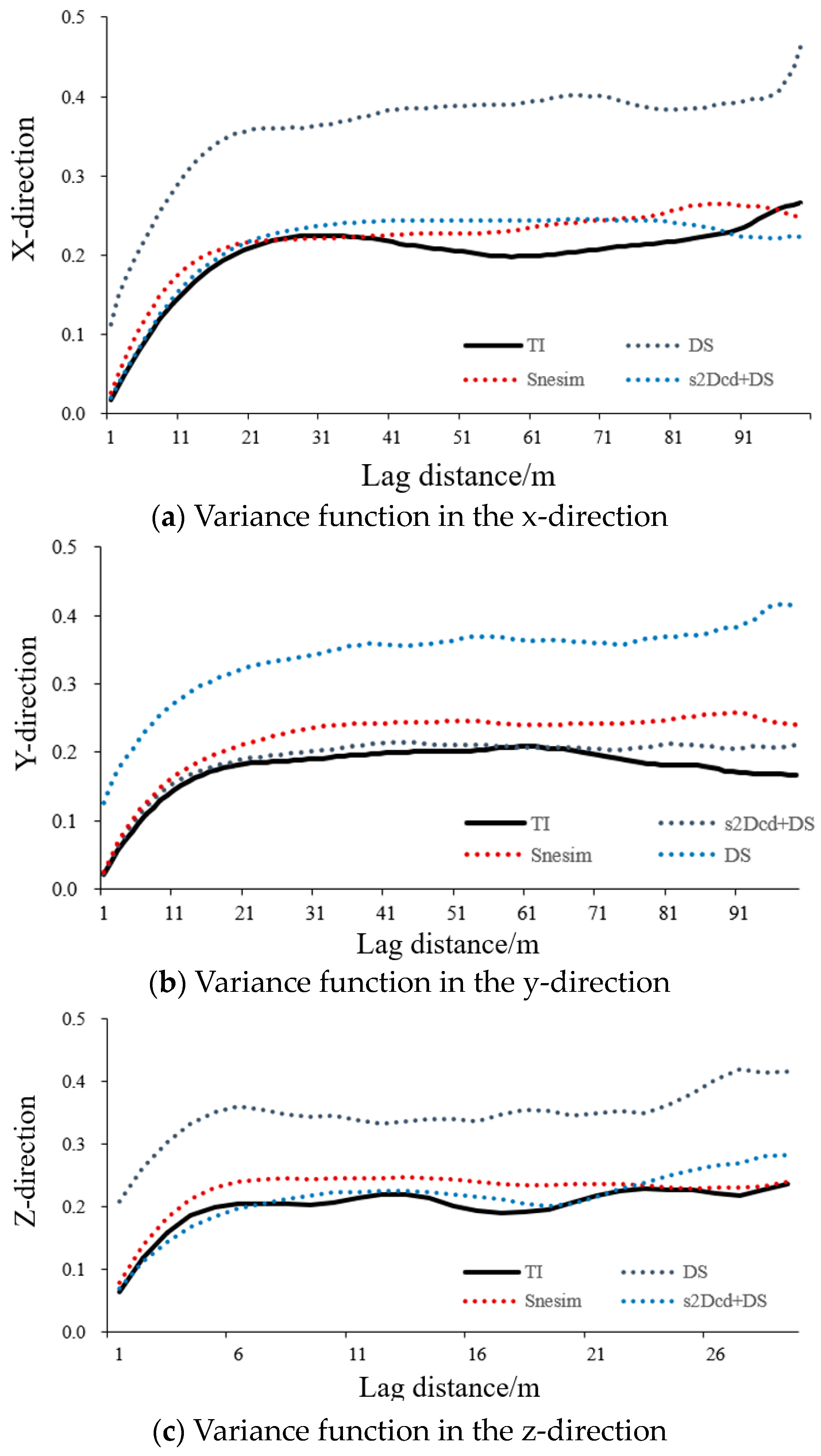
3.1. Variance Function

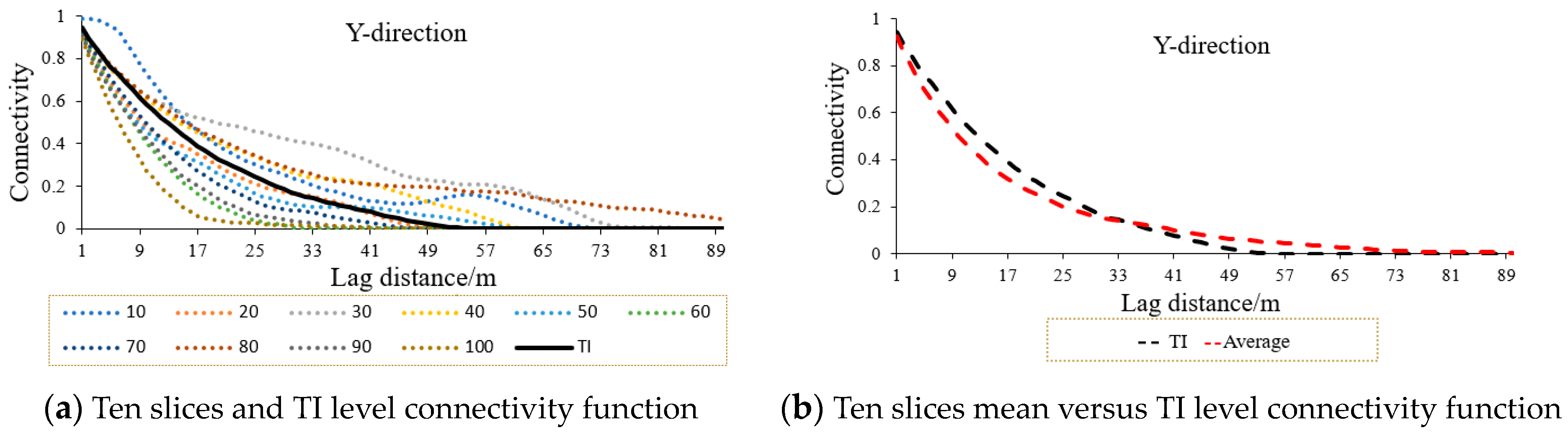
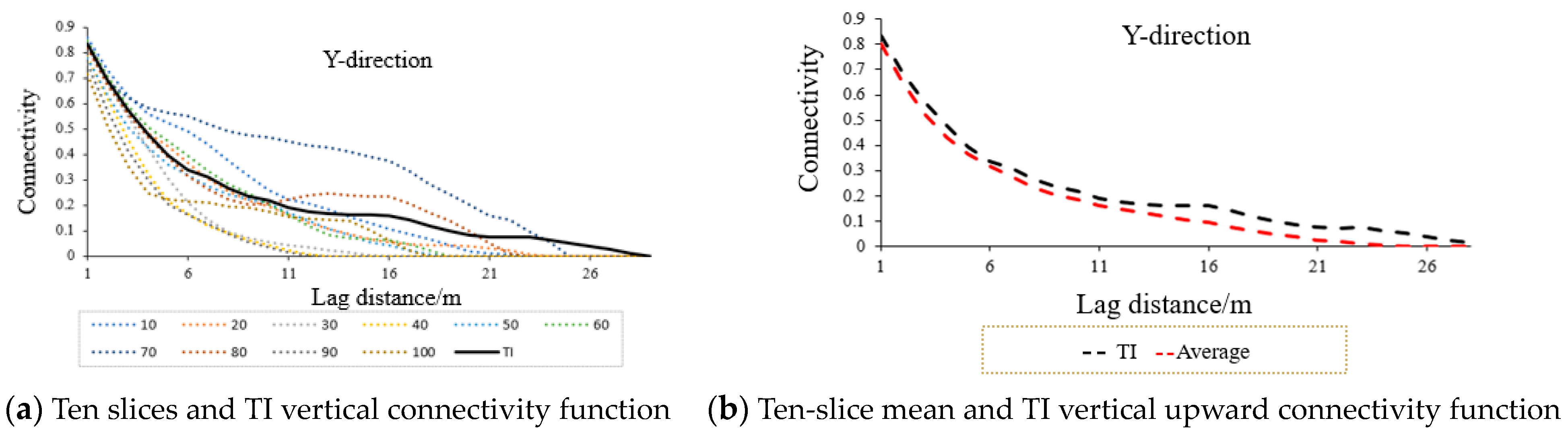
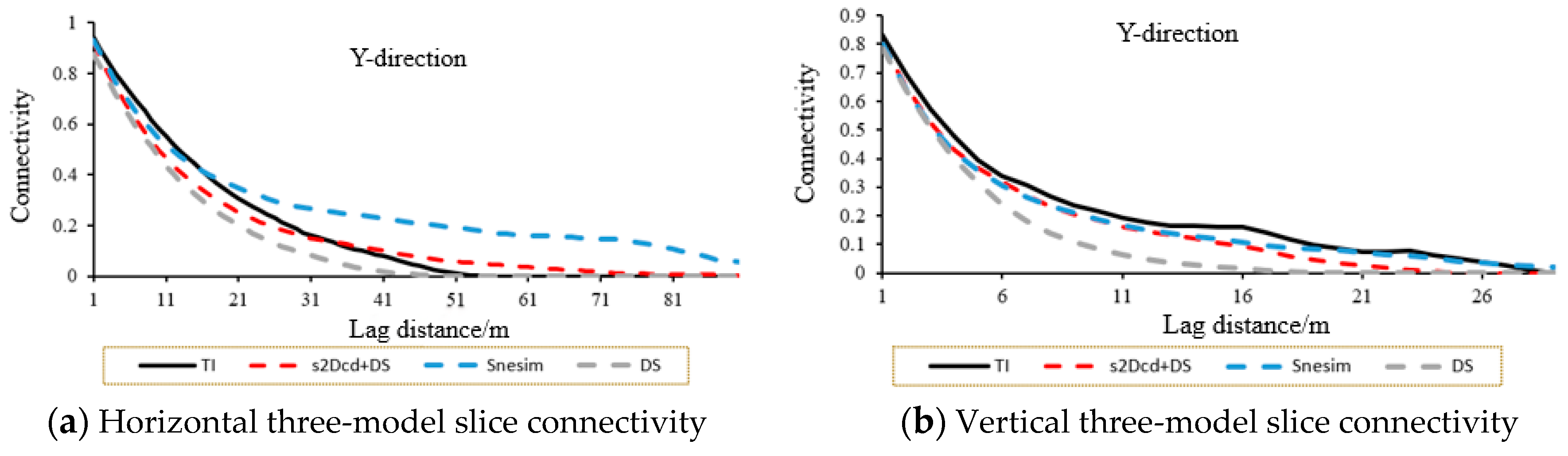
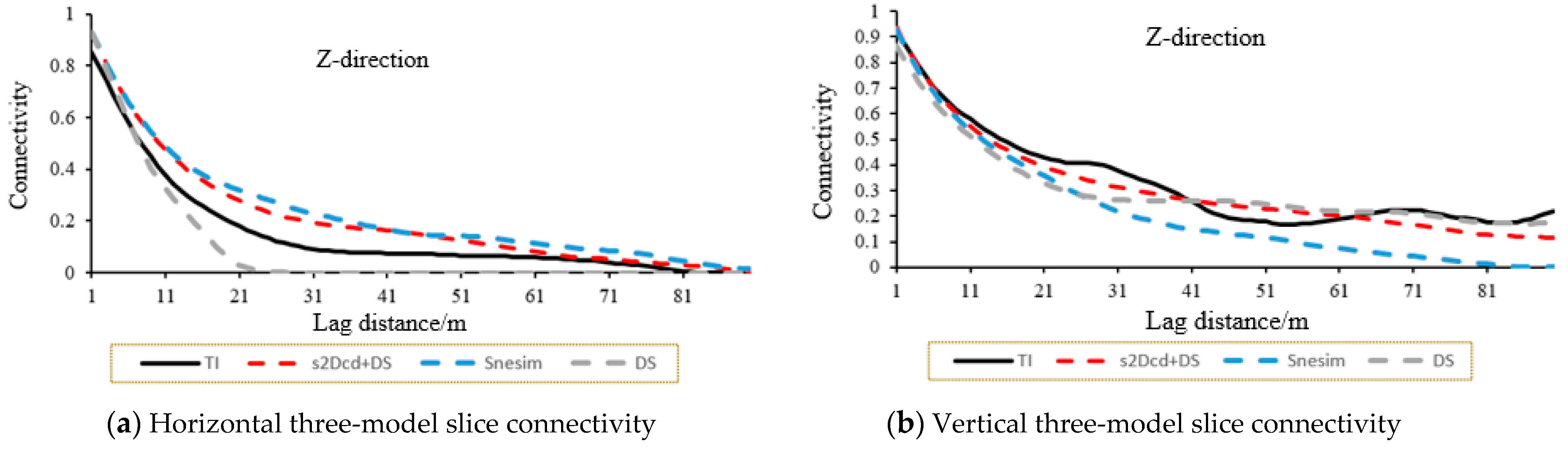
In order to evaluate the spatial variation characteristics of the algorithms in this paper, the 3D models generated by the above three algorithms were first evaluated in terms of the variance function with the original training images in the x-, y-, and z-directions. The variance functions are shown in Figure 7.

From the figure, it can be seen that Snesim and the algorithm in this paper basically match the variance function of the original training image, while DS is far from it, reflecting that the algorithm in this paper can obtain higher-order statistics and accurately reproduce the basic statistical information and heterogeneous features of the training image through the 3D model generated by 2D slicing.

3.2. Connectivity

Connectivity can reflect the degree of variation in the probability of connectivity of regionalized variables at a certain distance in a certain direction. In this paper, the idea of connectivity evaluation is borrowed from Nils Gueting et al. [21]. Nils Gueting used the training images produced by 2D ground-penetrating radar to simulate the generation of a 3D subsurface aquifer structure. One of the evaluation methods is to decompose the simulated 3D body into 2D vertical slices and calculate the MPH (multiple-point histogram). MPH indicates the frequency of spatial patterns in the grid and aims to reproduce the spatial features in the training image comparatively; the smaller the distance, the more consistent the spatial structure, and the better the simulation result; the larger the distance, the more inconsistent the structure, and the poorer the simulation result. The MPH of the training image is used as a reference, and the deviation of the simulation result MPH from it is quantified, thus providing information about the quality of the simulation result. Therefore, the 3D models generated by the above three algorithms were evaluated in terms of connectivity with the original training images in the x-, y-, and z-directions. The connectivity is calculated as:

$$\begin{gathered} K\left(h;n\right)=E\left\{I\left(u\right)I\left(u+h\right)\dots I\left(u+nh\right)\right\}=Prob\{I\left(u\right)=1,I\left(u+h\right) \\ =1,\dots ,I\left(u+nh\right)=1\} \end{gathered}$$

(1)

where h is a unit vector in any given direction and K(h; n) denotes the probability of observing n consecutive points. I(u) is the property at point u. When I(u) = 1, it represents that point u is a sand body; when I(u) = 0, it represents that point u is mud.

The steps of connectivity evaluation are: (1) First, slice the above three 3D models and find the connectivity curves of the sandstone in the models. Each slice contains the connectivity curves in horizontal and vertical directions. (2) Select 3 groups of 10 slices for each 3D model with equal spacing in the x-, y-, and z-directions. Find the connectivity of the sandstone in each direction in the three groups of models and find its mean value. (3) Compare the changes in the connectivity of the sandstone in the three directions in each group of models with the training images.

(1) The algorithm in this paper is used to generate the y-direction connectivity of the 3D model as an example (Figure 8). Ten slices with positions of y = 10, 20, 30, 40, 50, 60, 70, 80, 90, and 100 are selected in the y-direction of the 3D model, and the horizontal and vertical connectivity of each slice is found with equal spacing, as shown in Figure 8 and Figure 9. The connectivity curves of the 10 slices in the y-direction basically match with the training image, confirming that the 3D model generated from the 2D slices can obtain higher-order statistics while obtaining spatial correlation and location distribution features similar to those deposited in the training images.

(2) The connectivity of the x-, y-, and z-directions of the fluvial facies model generated by the method in this paper is compared with the methods of Snesim and DS, and the connectivity functions in each direction are found in the same way as in (1). The locations of equal intervals were selected: x = 10, 20, 30, 40, 50, 60, 70, 80, 90, 100. The slice sizes in the y-direction were the same as in (1), z = 3, 6, 9, 12, 15, 18, 21, 24, 27, 30, and the probability curves of sandstone connectivity in the three directions were compared as follows:

Figure 10 shows the comparison of the connectivity of the sandstone in the x-direction. Figure 10a shows the connectivity curves with different lag distances in the horizontal direction, and it can be seen that the method in this paper is in suitable agreement with the Snesim connectivity function, while the DS method generates the model with the largest difference in connectivity with the training images.

Figure 11 shows the comparison of the connectivity of sandstone in the y-direction. Figure 11a shows the connectivity curves of different lag point pairs in the horizontal direction and the best agreement between the method and TI in this paper; Figure 11b shows that the comparison of vertical connectivity and the connectivity curves of the method, TI, and Snesim in this paper are similar, and the deviation of DS and TI is relatively large.

Figure 12 shows the comparison of the connectivity of sandstone in the z-direction, and Figure 12a shows the connectivity curves of different pairs of lag point pairs in the horizontal direction, from which it can be seen that the connectivity curves of this paper and the Snesim method are similar, and the overall trend is similar to that of TI, and the s2Dcd+DS method is closer to the horizontal connectivity of the training image in the z-direction. The s2Dcd+DS method no longer has connectivity at the lag distance of 23, and the overall trend differs significantly from the training image. Figure 12b shows the comparison of vertical connectivity. The connectivity curves of the method, DS, and Snesim in this paper are similar to the training images and converge approximately.

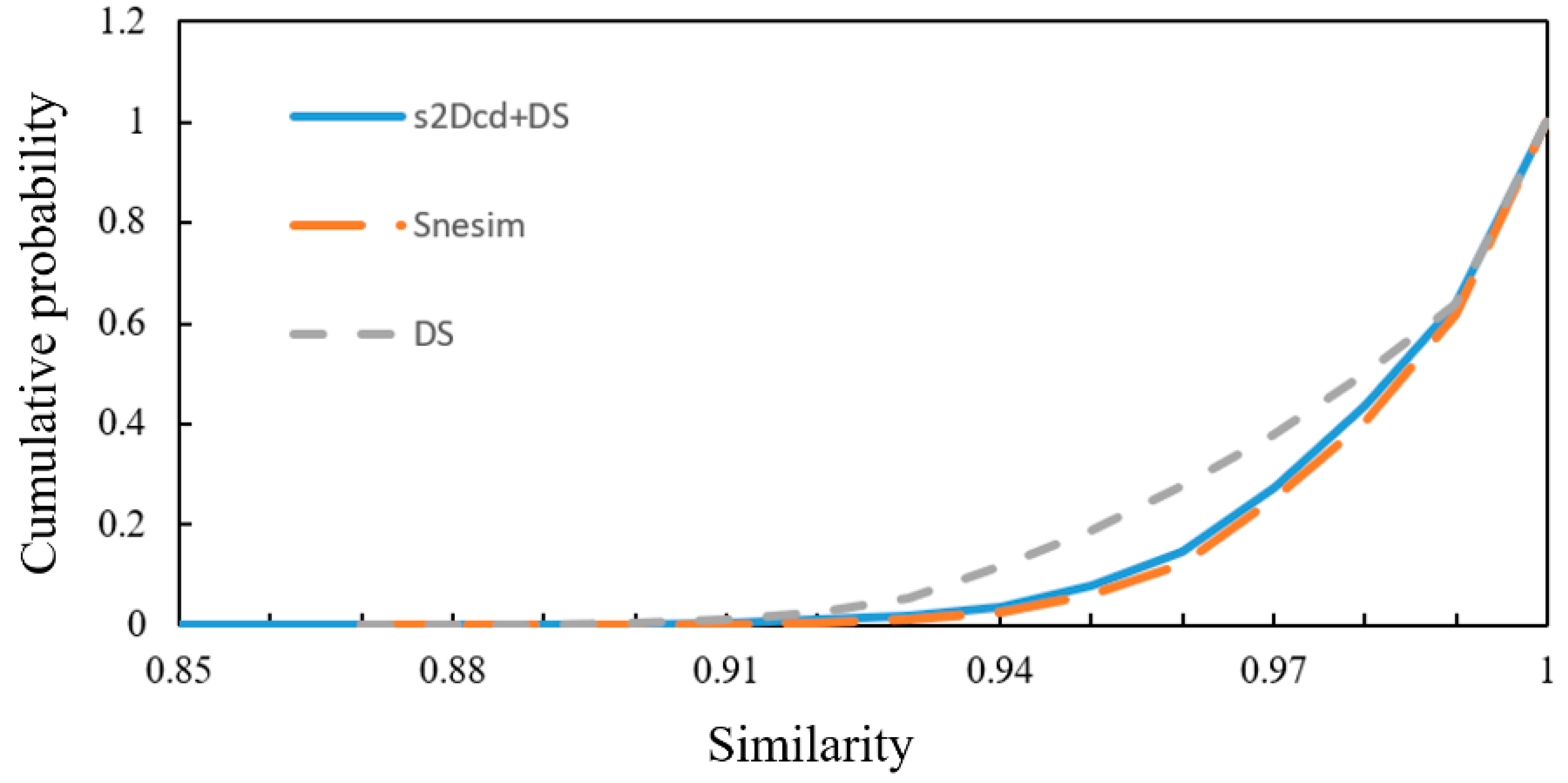
3.3. Style Similarity

A style database was constructed for each of the three sets of models and the original 3D training images. The similarity between the generated models and the training images was calculated, and the cumulative probability distribution function of the similarity calculation scores was calculated.

In the probability cumulative distribution plot, the lower the fitted curve is, the higher the similarity with the training images, and the higher the fitted curve is, the lower the similarity is [22]. As shown in Figure 13, the results obtained using the new method are similar to Snesim and superior to the DS-only method, confirming that the method in this paper can reproduce the data style well without using the 3D training images.

The histogram of the probability distribution of the similarity calculation of the fluvial facies implemented by the s2Dcd+DS method is shown in Figure 14. From the mean, standard deviation, and median of the histograms, it can be seen that the model reproduction rate deviation of the simulation implementation results of the method in this paper is small, indicating that the conditional simulation implementation of the two fluvial facies types can reproduce the training image a priori geological model better.

4. Conclusions

(1)

Previously, in the direction of digital cores, the target-based method, process-based method, simulated annealing method, and stochastic modeling method were applied to construct 3D training images using 2D training images, and it is difficult to apply these methods to construct 3D training images in the direction of reservoir modeling. To overcome this difficulty, the new algorithm in this paper integrates the s2Dcd algorithm and DS algorithm, combining the advantages of sequential 2D conditional simulation and direct sampling simulation methods. In this paper, the new algorithm combines the advantages of sequential two-dimensional conditional simulation and direct sampling simulation methods, weakens the influence of conditional data, reduces the simulation error, and realizes the construction of a three-dimensional fluvial facies reservoir model based on two-dimensional training images.

(2)

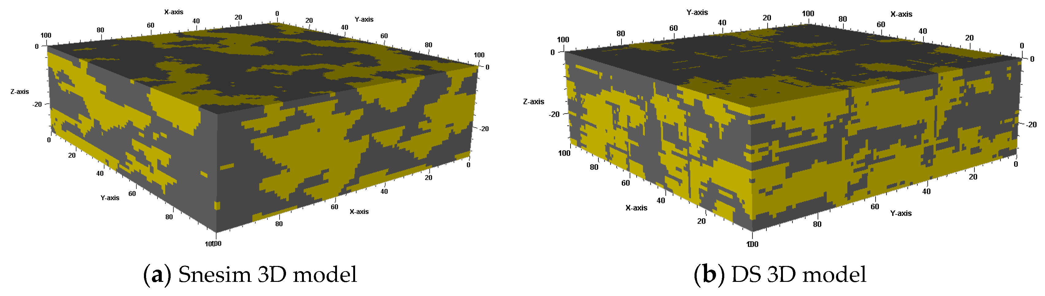
By comparing the variance functions, the horizontal and vertical connectivity in the x-, y-, and z-directions, and the style similarity, the results show that the new modeling method proposed in this paper can achieve the effect of approximate direct 3D training image based on several mutually perpendicular 2D training images, using multiple slices to realize the conditional simulation of the fluvial facies model. In the case where it is difficult to obtain 3D training images, the new modeling method proposed in this paper has suitable prospects for application in the direction of reservoir modeling.

(3)

We have been on the way to training image reconstruction, and multipoint geostatistics has been developing. The new method in this paper is difficult to obtain 3D training images in the direction of reservoir modeling and has a suitable application prospect. We hope that in the near future, our methods will become more and more advanced and provide great value for reservoir recovery.

References

1. Wang, K.; Xiao, F. Multiple-Points Geostatistics: A Review of Theories, Method and Applications. J. Geol. Sci. Technol. Intell. 2019, 38, 256–268. [Google Scholar] [CrossRef]
2. Yu, M. Construction and Application of Multi-Point Geostatistics 3D Training Image for the Calculation of Bread Mineral Resources. Master’s Thesis, Jiangxi University of Science and Technology, Ganzhou, China, 2022. [Google Scholar] [CrossRef]
3. Yang, P. Geostatistics inversion—From two-point to multiple-point. Prog. Geophys. 2014, 29, 2293–2300. (In Chinese) [Google Scholar]
4. Wang, M.; Shang, X.; Duan, T. A Review of the Establishment Methods of Training Image in Multi-point Statistics Modeling. Geol. J. China Univ. 2022, 28, 96103. [Google Scholar] [CrossRef]
5. Chen, J.Y.; Yu, X.H.; Zhang, Z.J.; Li, L.S.; Mao, Z.G. Application of reservoir geological modeling in reservoir description. Daqing Pet. Geol. Dev. 2005, 24, 17–18. [Google Scholar]
6. Hu, X.; Xiong, Q.; Wu, S. Research progress of reservoir modeling methods. J. Univ. Pet. (Nat. Sci. Ed.) 2001, 25, 107–112. [Google Scholar]
7. Hidajat, I.; Rastogi, A.; Singh, M.; Mohanty, K.K. Transport Properties of Porous Media Reconstructed from Thin-Sections. SPE J. 2002, 7, 40–48. [Google Scholar] [CrossRef]
8. Keehm, Y.; Mukerji, T.; Nur, A. Permeability prediction from thin sections: 3D reconstruction and Lattice-Boltzmann flow simulation. Geophys. Res. Lett. 2004, 31. [Google Scholar] [CrossRef]
9. Zhu, Y.; Tao, G.; Fang, W. Application of image processing technology in digital core modeling. J. Oil Gas Technol. 2007, 101, 54–57+166. [Google Scholar]
10. Liu, X.-F.; Zhang, W.-W.; Sun, J.M. Methods of constructing 3-D digital cores: A review. Prog. Geophys. 2013, 28, 3066–3072. (In Chinese) [Google Scholar] [CrossRef]
11. Wang, Z. Application of modern sedimentary and close well pattern data building training image in phase modeling. China Pet. Chem. Stand. Qual. 2018, 38, 121–122. [Google Scholar]
12. Bao, H.S.; Han, T.C.; Fu, L.Y. Calculation method of digital rock electrical conductivity based on two-dimensional images. Chin. J. Geophys. 2021, 64, 1733–1744. (In Chinese) [Google Scholar] [CrossRef]
13. Liang, Z.; Ioannidis, M.A.; Chatzis, I. Permeability and electrical conductivity of porous media from 3D stochastic replicas of the microstructure. Chem. Eng. Sci. 2000, 55, 5247–5262. [Google Scholar] [CrossRef]
14. Mo, X.W.; Zhang, Q.; Lu, J.A. A complement optimization scheme to establish the digital core model based on the simulated annealing method. Chin. J. Geophys. 2016, 59, 1831–1838. (In Chinese) [Google Scholar] [CrossRef]
15. Comunian, A.; Renard, P.; Straubhaar, J. 3D multiple-point statistics simulation using 2D training images. Comput. Geosci. 2012, 40, 49–65. [Google Scholar] [CrossRef] [Green Version]
16. Mariethoz, G.; Renard, P. Reconstruction of Incomplete Data Sets or Images Using Direct Sampling. Math. Geosci. 2010, 42, 245–268. [Google Scholar] [CrossRef] [Green Version]
17. Geng, L.; Hou, J.; Li, Y.; Li, Z.; Qu, P. Application of DS-MPS Algorithm in the Modeling of Reservoir Sedimentary Facieses. Pet. Geol. Oilfield Dev. Daqing 2015, 34, 24–29. [Google Scholar]
18. Liu, Y. Research progress of multi-point geostatistics in fluvial facies modeling. Sci. Technol. Inf. 2012, 160–161. [Google Scholar]
19. Wu, S.; Jin, Z.; Huang, C.; Chen, C. Reservoir Modeling; Petroleum Industry Press: Beijing, China, 1999. [Google Scholar]
20. Wang, J.; Zhang, T. Stochastic Modeling of Oil and Gas Reservoir; Petroleum Industry Press: Beijing, China, 2001. [Google Scholar]
21. Gueting, N.; Caers, J.; Comunian, A.; Vanderborght, J.; Englert, A. Reconstruction of Three-Dimensional Aquifer Heterogeneity from Two-Dimensional Geophysical Data. Math. Geosci. 2018, 50, 53–75. [Google Scholar] [CrossRef] [Green Version]
22. Yu, S.; Li, S.; Wang, D.; Wang, J.; Zhang, Y.; Yu, J. Multipoint geo-statistical modeling algorithm based on p-stable LSH. Acta Pet. Sincia 2017, 38, 1425–1433. [Google Scholar]
Figure 1. s2Dcd condition simulation flowchart.
Applsci 13 07497 g001
Figure 2. Geographical location map of the study area.
Applsci 13 07497 g002
Figure 3. Training images of discrete channel courses.
Applsci 13 07497 g003
Figure 4. Well condition data of channel sand body.
Applsci 13 07497 g004
Figure 5. Simulation results of fluvial facies conditioning.
Applsci 13 07497 g005
Figure 6. Three−dimensional model.
Applsci 13 07497 g006
Figure 7. Generated model with 3D TI as a function of variance in three directions.
Applsci 13 07497 g007
Figure 8. Connectivity on the Y-direction slice level.
Applsci 13 07497 g008
Figure 9. Y-directional slice vertical upward connectivity.
Applsci 13 07497 g009
Figure 10. Connectivity in the x-direction.
Applsci 13 07497 g010
Figure 11. Connectivity in the y-direction.
Applsci 13 07497 g011
Figure 12. Connectivity in the z-direction.
Applsci 13 07497 g012
Figure 13. Cumulative probability distribution of similarity of different methods.
Applsci 13 07497 g013
Figure 14. Probability histogram of similarity calculation of conditionalized sand body model.
Applsci 13 07497 g014