Comparison of Damage Indexes for Assessing Seismic Fragility of Bearings in an Offshore Bridge

Abstract

This study analyzes the applicability of different damage indexes for bearings, focusing on the time-dependent deterioration of materials and the time-dependent bond-slip behavior between steel and concrete caused by chloride erosion. First, the methodology is proposed, encompassing the time-dependent deterioration of materials, the time-dependent bond-slip behavior, the quantification of different damage indexes of the bearing, and the fragility analysis for the bearings. Next, an offshore bridge is used as an example to investigate the detailed elements of the components and the time-varying effects. Thereafter, based on incremental dynamic analysis and fragility analysis, the discussion focuses on the comparison of damage indexes for assessing the seismic fragility of bearings in an offshore bridge. This study indicates that if the relative displacement ductility ratio is adopted as the criterion, the coverage of PGA obtained by the theoretical method is 167% greater than that obtained using the empirical method, and the relative displacement ductility ratio, which incorporates the shear deformation of piers, is better aligned with the performance-based ductility design concept and offers better economy. Safety-based damage indexes are recommended for the bridge in seismic zones, while economy-based indexes can be used in favorable bridge environments.

1. Introduction

Bridge bearings are important components in the seismic analyses of bridge structures. They are also one of the most fragile components under earthquakes [1]. Although bearings are replaceable throughout the operational lifespan of the bridge, their damage during the replacement period can seriously affect the normal serviceability of bridges. Therefore, it is necessary to analyze the dynamic response of bearings and quantify and classify their damage state under earthquakes.

Previous studies proposed various methods for defining the damage states of bearings. These methods are based on different parameters, such as relative displacement, shear strain, and relative displacement ductility ratio. Hwang, Liu [2] defined a damage index for a neoprene bearing pad by considering the shear force of the bearing as the demand parameter. They then presented an analytical method for the development of fragility curves of highway bridges based on the classification of the damage state. Nielson [3] updated damage index limits for movable and fixed steel bearings using a Bayesian theory. After that, scholars further updated the quantification method of damage states for bearings based on the displacement under the earthquake-induced excitation, encompassing the shear strain, displacement, and displacement angle. Among them, Zhang and Huo [4] proposed classification criteria for different damage states under earthquakes using shear strain, displacement, and displacement angle. Furthermore, the establishment of damage criteria for bearings aimed to establish a relationship between the response quantities of the components and the overall damage states of bridges. A damage index was proposed by Wu, Li [1], which is using the displacement and displacement ductility ratio values corresponding to different damage states. They found that such bridges’ bearings are more susceptible to earthquakes than piers and abutments, especially the movable bearings at the abutments. Alam, Bhuiyan [5] proposed damage indexes for elastomeric pads and sliding bearings and analyzed the earthquake resistance of a highway bridge retrofitted with laminated rubber bearings and shape memory alloy (SMA) restrainers.

To improve the precision of evaluating the impact of bearings on the operational reliability of bridges subjected to seismic activity, researchers such as Shinozuka, Feng [6], Hwang, Liu [2], and Nielson [3] proposed a fragility analysis theory based on traditional reliability theory. This theory employs a joint failure probability analysis method to investigate the earthquake resistance for the components and their implications for the operational characteristics of structural systems. Parool and Rai [7] analyzed the fragility curves for bearings along two horizontal directions and provided solutions for retrofitting existing bridges. Furthermore, Taskari and Sextos [8] conducted a seismic fragility analysis and found that movable steel bearings are highly vulnerable to failure under seismic excitation.

Recent developments in research on fragility analyses of bearings showed the significant influence of time-varying deterioration of materials on the operational effectiveness of bearings. Liang, Yan [9] and Liang, Yan [10] conducted an analysis of the seismic behavior of bearings in offshore bridges based on their relative displacement. Their findings indicate that material deterioration leads to an increase in the dynamic response and failure probability of bearings under earthquake loading. Moreover, Ghosh and Padgett [11] discovered that the peak deformation of bearings increases significantly when an aging factor is taken into account. The effect of corroded steel bearings on the component-level seismic fragility of a bridge was examined by Shekhar and Ghosh [12]. Their study emphasized the significance of using realistic bearing degradation models for bridges located in seismic regions that experience corrosion deterioration.

There was a lack of attention paid to the comparative analysis of the differences between various methods of quantifying damage indexes. See details in

Table 1. Literature review of damage indexes for the bearings.

Theme	Year	Main Contribution
Definitions of damage state	2001	Hwang, Liu [2] defined a damage index for a neoprene bearing pad.
	2005	Nielson [3] updated damage index limits for movable and fixed steel bearings.
	2009	Zhang and Huo [4] proposed classification criteria for different damage states using the shear strain, displacement angle, and displacement.
	2016	Wu, Li [1] proposed a damage index using a displacement ductility ratio and displacement for a plate rubber bearing and polytetrafluoroethylene (PTFE) sliding plate bearing.
	2012	Alam, Bhuiyan [5] proposed damage indexes for elastomeric pads and sliding bearings.
Assessment of the seismic performance	2000, 2001, and 2005	Shinozuka, Feng [6], Hwang, Liu [2], and Nielson [3] proposed a fragility analysis theory based on traditional reliability theory.
	2014	Parool and Rai [7] analyzed the fragility curves for bearings along two horizontal directions.
	2015	Taskari and Sextos [8] conducted a seismic fragility analysis of the movable steel bearings.
Durability damage	2020 and 2021	Liang, Yan [9] and Liang, Yan [10] found that material deterioration leads to an increase in the seismic response and failure probability of bearings.
	2010	Ghosh and Padgett [11] discovered that the peak deformation of bearings increases significantly when an aging factor is taken into account.
	2018	Shekhar and Ghosh [12] highlighted the importance of realistic bearing degradation models for bridges.

. Additionally, there is no systematic approach among the different quantification methods. Therefore, this study proposes a new method for quantifying damage indexes of bearings based on incremental dynamic analysis and fragility analysis. The proposed method is validated using a numerical model of an offshore bridge. The results show that the proposed method is able to accurately predict the damage state of bearings under seismic loading. This paper is structured in the following manner: Section 2 presents the theoretical model, which includes the time-varying durability analysis for materials, the effect of time-dependent bond-slip, the quantification of different damage indexes of the bearing, and the fragility analysis method of the bearing. Section 3 introduces the nonlinear finite element model for the bridge. Section 4 discusses the comparison of damage indexes for assessing the seismic fragility of bearings in an offshore bridge. Finally, Section 5 presents the overall discussions and main findings of this study.

2. Methodology

2.1. Time-Dependent Deterioration of Materials

Reinforced concrete structures consist of concrete and reinforcement, and their performance relies on the properties of both materials. The mechanical behavior of these materials, particularly concrete and reinforcement, must be fully considered using suitable constitutive models.

Concrete piers are comprised of both confined and unconstrained concrete. The unconstrained concrete serves as a protective layer for the piers, while the confined concrete in the core area is reinforced by longitudinal reinforcement and stirrups to increase its strength and durability. The constitutive relationship for the concrete adopts the Kent–Park model (Concrete 01) (Kent and Park 1990, [9,10]), and the mechanical properties of the confined concrete are as shown in Equations (1)–(6) [9,13,14].

$$\left\{\begin{array}{l}{x}_c=k\cdot \sqrt{t}\\ \overline{S}=\raisebox{1ex}{$A_c$}\!\left/ \!\raisebox{-1ex}{$A$}\right.\end{array}\right.$$

(1)

$${\sigma }_{cp}=(1+0.619\cdot \overline{S})\cdot {\sigma }_p$$

(2)

$${\epsilon }_{cp}=(1-0.106\cdot \overline{S})\cdot {\epsilon }_p$$

(3)

$${\epsilon }_{cu}=(1-0.459\cdot \overline{S})\cdot {\epsilon }_u$$

(4)

$$E_c=(1+0.503\cdot \overline{S})\cdot E$$

(5)

$$G_c=\frac{E_c}{2\cdot (1+\mu )}$$

(6)

where k, $\overline{S}$, and t are the carbonation coefficient, carbonation rate, and carbonation time, respectively. A_c is the area of carbonation. A is the area of total cross-sectional, x_c is the depth of carbonation, σ_p, ε_p, ε_u, and E are peak stress, peak strain, ultimate strain, and elastic modulus of concrete before carbonation, respectively, σ_cp, ε_cp, ε_cu, E_c, and G_c are peak stress, peak strain, ultimate strain, elastic modulus, and shear modulus of carbonated concrete, respectively, and μ is Poisson’s ratio.

Steel 02 possesses an isotropic strain hardening property and accurately represents both the bi-directional Bauschinger effect and isotropic strengthening effect. In the works of Liang, Yan [10], Wu, Li [15], and Sung and Su [16], the calculations for the corrosion initiation time of the reinforcement, chloride ion concentration on the concrete surface, yield strength, and elastic modulus of reinforcement are provided as shown in Equations (7)–(12). For more details, the reader can refer to Yan, Liang [17], and Liang, Yan [10].

$$t_i\prime ={\left(\frac{c}{K}\right)}^2\times {10}^{-6}$$

(7)

$$t_i=t_i^{\prime }+0.2t_1$$

(8)

$$t_{cr}=t_i+t_c$$

(9)

$$t_c=\frac{{\delta }_{cr}}{{\lambda }_{cl}}$$

(10)

$$f_{yc}=\left(1-0.339\rho \right)\cdot f_y$$

(11)

$$E=\left(1-1.166\rho \right)\cdot E_s$$

(12)

where t_i and t’_i are the corrosion initiation time for the reinforcement (year), taking into account and disregarding the chloride erosion, respectively; t₁ the cumulative duration (year) required for chloride ions to reach a stable concentration on the surface of the concrete; t_cr and t_c are the time (year) for concrete cracking and time (year) from the initiation of steel corrosion to concrete cracking; c is the concrete cover thickness (mm); K is the coefficient of chloride penetration (m²/year); E and E_s are the elastic moduli of the corroded and non-corroded reinforcement, respectively (MPa); f_yc and f_y are the yield strengths of the corroded and non-corroded reinforcement, respectively (MPa); δ_cr is the corrosion depth for the steel when the concrete cracks (mm); and λ_cl is the annual average corrosion rate for the steel before the concrete cracks (mm/year), as shown in

Table 2. Time-varying effects on the concrete’s material properties.

Time (Year)	Peak Stress (MPa)		Peak Strain (ε)		Ultimate Strain (ε)		Elastic Modulus (MPa)
	C40	C50	C40	C50	C40	C50	C40	C50
0	34.00	42.50	−0.002000	−0.002000	−0.004000	−0.004000	32,500.00	34,500.00
30	34.18	42.60	−0.001999	−0.001999	−0.003988	−0.003993	32,609.50	34,567.39
50	34.21	42.63	−0.001998	−0.001999	−0.003984	−0.003991	32,640.59	34,587.04
70	34.24	42.66	−0.001998	−0.001999	−0.003981	−0.003989	32,666.78	34,602.83
100	34.26	42.69	−0.001997	−0.001999	−0.003978	−0.003987	32,699.55	34,623.32

and

Table 3. Time-varying effects on the reinforcement’s material properties.

Time (Year)	Diameter (mm)				Yield Strength (MPa)				Elastic Modulus (×105 MPa)
	C50		C40		C50		C40		C50		C40
	L	S	L	S	L	S	L	S	L	S	L	S
0	32.00	16.00	32.00	16.00	335.00	235.00	335.00	235.00	2.00	2.10	2.00	2.10
30	31.92	15.70	31.76	15.67	334.43	232.07	333.30	231.75	1.99	2.01	1.97	2.00
50	31.65	15.29	31.54	15.26	332.53	228.10	331.72	227.85	1.95	1.89	1.93	1.88
70	31.36	14.88	31.26	14.86	330.51	224.24	329.78	224.05	1.91	1.77	1.89	1.76
100	30.93	14.26	30.79	14.25	327.56	218.65	326.56	218.54	1.85	1.60	1.83	1.59

L and S are chosen to denote the longitudinal reinforcement and stirrup, respectively.

.

The Kent–Park model is a bilinear model that captures the behavior of concrete in both the elastic and plastic ranges. The model is based on the stress–strain relationships for concrete in tension and compression. The model is also able to account for the effects of carbonation on the mechanical properties of concrete. The mechanical properties of the confined concrete are determined by the properties of the unconfined concrete and the reinforcement. The reinforcement provides confinement to the concrete, which increases its strength and ductility.

The time-varying durability analysis of materials is used to predict the degradation of the materials over time. The degradation is caused by a number of factors, including environmental factors such as moisture and chlorides, and loading factors such as cyclic loading. The degradation can lead to a decrease in the strength and durability of the materials, which can in turn lead to a decrease in the performance of the structure. The time-varying durability analysis of materials is an important part of the design of reinforced concrete structures. The analysis can be used to identify the critical areas of the structure and to select the appropriate materials and reinforcement for those areas. Table 2 and Table 3 present the time-varying effects on the concrete’s material properties and the time-varying effects on the reinforcement’s material properties, respectively.

2.2. Time-Dependent Bond-Slip Behavior

As we know, the reinforcement provides strength and ductility through their anchorage to concrete. However, during the service life, the reliability of this connection will gradually decrease as the reinforcement and concrete materials degrade. In other words, with an increase throughout the operational lifespan of the bridge, the deterioration of the concrete and reinforcement will cause the mechanical properties to continue to decrease, and a large amount of rust accumulation will be formed in the contact interface between the reinforcement and concrete, reducing the bonding effect of the concrete to the reinforcement [18]. Therefore, the bond-slip is selected as the evaluation index for the bond strength degradation, and the “Strain Penetration Model for Fully Anchored Steel Reinforcing Bars” is selected to model the bond-slip behavior [19], see Equation (13) for more details. Figure 1 shows the relationship between the yield strength and corrosion rate of the longitudinal reinforcement and rising rate of the bond-slip for C40 concrete (piers 1#, 2#, and 5#) during its entire life cycle.

$$S_y(mm)=2.54\times {\left[\frac{d_b(mm)}{8437}\frac{f_y(MPa)}{\sqrt{f_c\prime (MPa)}}\times (2\alpha +1)\right]}^{1/\alpha }+0.34$$

(13)

where f_y and f_c’ are the reinforcement yield strength and concrete peak compressive stress, respectively; d_b is the longitudinal reinforcement diameter; α is the bond-slip coefficient, typically assumed to be 0.4. The command for “Strain Penetration Model for Fully Anchored Steel Reinforcing Bars” creates a uniaxial material object to capture strain penetration effects at various intersections, such as column-to-footing, column-to-bridge bent caps, and wall-to-footing connections. In these scenarios, bond-slip occurs along a section of the anchorage length due to strain penetration. The model can also be applied to beam end regions where strain penetration may involve bar slippage along the entire anchorage length, provided appropriate model parameters are chosen. This model specifically addresses fully anchored steel reinforcement bars that experience bond-slip within a portion of the anchorage length due to strain penetration effects. Such effects are commonly observed in situations where column and wall longitudinal bars are anchored into footings or bridge joints.

As the service life of the bridge increases, Figure 1 indicates that the yield strength of the longitudinal reinforcement deteriorates with the increase in the corrosion rate of the longitudinal reinforcement. Among them, the yield strengths after 30, 50, 70, and 100 years are reduced by 0.51%, 0.98%, 1.56%, and 2.52%, respectively. Additionally, as the operational lifespan of the structure increases, the bond-slip and its rising rate increase with the corrosion rate of longitudinal reinforcement. Apparently, the rising rate in bond-slip is greatest when the bridge is in service for 0–30 years, since the time for C40 concrete to crack to the surface of the longitudinal reinforcement is 27 years. When the service life of the bridge is 30–50 years, the rising rate decreases gradually. When the service life of the bridge is 50–100 years, the rising rate is basically saturated; in other words, the bond-slip starts to increase at a steady rate.

As can be seen from the figure, the rising rate of the bond-slip increases with the decrease in the yield strength and increase in the corrosion rate of the reinforcement. This is because the lower the yield strength of the reinforcement, the easier it is for the reinforcement to be corroded. The higher the corrosion rate of the reinforcement, the more rust accumulation there is in the contact interface between the reinforcement and concrete, which weakens the bond and anchoring effect of concrete to the reinforcement. The time-dependent bond-slip behavior is an important factor that needs to be considered in the design of reinforced concrete structures. The model presented in this section can be used to calculate the bond-slip relationship between the reinforcement and concrete as a function of the yield strength and corrosion rate of the reinforcement. This information can be used to design the reinforcement and concrete to ensure that the structure has the required strength and ductility.

2.3. Definition of Damage Indexes for Bearings

A crucial aspect in assessing the fragility of a structure is determining its damage state under an earthquake based on a performance level and quantifying the damage index under different damage states. Hwang, Liu [2] found that the failure process of a structure can be described by five distinct damage states, namely: no damage, minor damage, medium damage, serious damage, and complete destruction. At present, there is no systematic theoretical standard for calculating a damage index for bearings. However, through the exploration of scholars in the past 20 years, the following three quantitative criteria can be obtained: (1) the relative displacement (Δx), i.e., the relative displacement between the bearing and pier top under earthquake action, (2) the shear strain (γ), i.e., the shear deformation of the bearing under earthquake action, and (3) the relative displacement ductility ratio (Δμ), i.e., the measure of the ability of the bearing to deform under earthquake action without sustaining damage. It is calculated as the ratio of the relative displacement to the shear strain. Equations (14)–(16) provide more details on how to calculate these three criteria.

$$\Delta x=\left|x_b-x_p\right|$$

(14)

$$\gamma =\frac{\Delta x_{max}}{t}$$

(15)

$$\Delta \mu =\frac{\Delta x_{max}}{{\Delta x}_{\gamma 100\%}}$$

(16)

where x_b is the bearing displacement (mm), x_p is the pier top displacement (mm), Δx_max is the maximum relative displacement of the bearing (mm), t is the bearing thickness (mm), and Δx_γ100% is the relative displacement (mm) at 100% shear strain of the bearing.

Taking the movable spherical steel bearing of the example bridge as an example, the definition of the damage state for the example bearing is described below, referring to the restoring force model of the PTFE slide bearing.

(1) Method 1: This method is based on the maximum allowable displacement of the bearing [20,21]. The bearing is considered to be undamaged if the displacement is less than or equal to half of the maximum allowable displacement. The bearing is considered to be damaged if the displacement is greater than half of the maximum allowable displacement. The severity of the damage is determined by the amount of displacement. As shown in Figure 2, Δx₁ is 1/2 of the maximum allowable displacement of bearing, Δx₂ is the maximum allowable relative displacement of bearing, which is the distance from the edge of the upper seat plate to the edge of the upper rotating surface, and Δx₃ is the distance between the outermost edge of the upper seat plate and the outer edge of the middle seat plate on the other side. This method is the most straightforward and easy to implement. However, it is also the least accurate. This is because the maximum allowable displacement is a conservative value that is based on the worst-case scenario. In most cases, bearings will not experience the maximum allowable displacement.

(2) Method 2: This method is based on the shear strain of the bearing [4]. The bearing is considered to be undamaged if the shear strain is less than or equal to 100%. The bearing is considered to be damaged if the shear strain is greater than 100%. The severity of the damage is determined by the amount of shear strain. This method is more accurate than Method 1. However, it is also more complex and difficult to implement. This is because the shear strain is a measure of the deformation of the bearing. The shear strain can be difficult to measure, especially in large bearings.

(3) Method 3: This method is based on the relative displacement ductility ratio of the bearing [22]. The bearing is considered to be undamaged if the relative displacement ductility ratio is less than or equal to μ₁. The bearing is considered to be damaged if the relative displacement ductility ratio is greater than μ₁. The severity of the damage is determined by the amount of the relative displacement ductility ratio. Among them, μ₁ is the relative displacement ductility ratio when the shear strain of the bearing is equal to 100%. This method is the most accurate of the three methods. However, it is also the most complex and difficult to implement. This is because the relative displacement ductility ratio is a measure of the ability of the bearing to deform without sustaining damage. The relative displacement ductility ratio can be difficult to measure, especially in large bearings.

The above three methods are summarized in Table 3 and Figure 3. The table shows the average values of the four algorithms for each method. The figure shows the relationship between the damage index and the displacement, shear strain, and relative displacement ductility ratio. It can be seen from the table and figure that the three methods are all effective in quantifying the damage index of a bearing. The method that is most suitable for a particular application will depend on the specific requirements of the application. Among them, for method 1, there are three situations: (1) Of the reference values given by scholars based on experience, there are currently three types (named B1–B3) widely used by scholars of bridge engineering. Additionally, the average value of the above three methods is also given here for comparative analysis, named A1. (2) Based on the quantification method proposed in Figure 2 (named B4), the damage index of each state is solved. (3) For comparison, the average values of the above four algorithms (B1–B4) are given, which is named A2. Method 2 is named B5. As for method 3, which is similar to method 1, there are three situations: (1) the reference values based on the experience of scholars are named B6–B9. Additionally, the average value of the above four methods is also given here for comparative analysis, named A3. (2) According to the quantification method proposed in Equation (18) (named B10), the damage index for each state can be determined. (3) For comparison, the average values of the above five algorithms (B6–B10) are given, named A4.

Among the existing methods for quantifying damage indexes of bearings, two main approaches exist:

(1) Empirical methods: provide reference values for the damage index based on the experience of scholars. These reference values are based on the observed damage to bearings after earthquakes.

(2) Theoretical methods: calculate the damage index based on the properties of the bearing and the earthquake loading. These methods are based on established theories and are therefore more accurate than empirical methods.

A detailed comparison and applicability analysis of the two quantification methods was conducted during the service life of the bearing when subjected to earthquakes.

As shown in

Table 4. Damage indexes of bearing under different types.

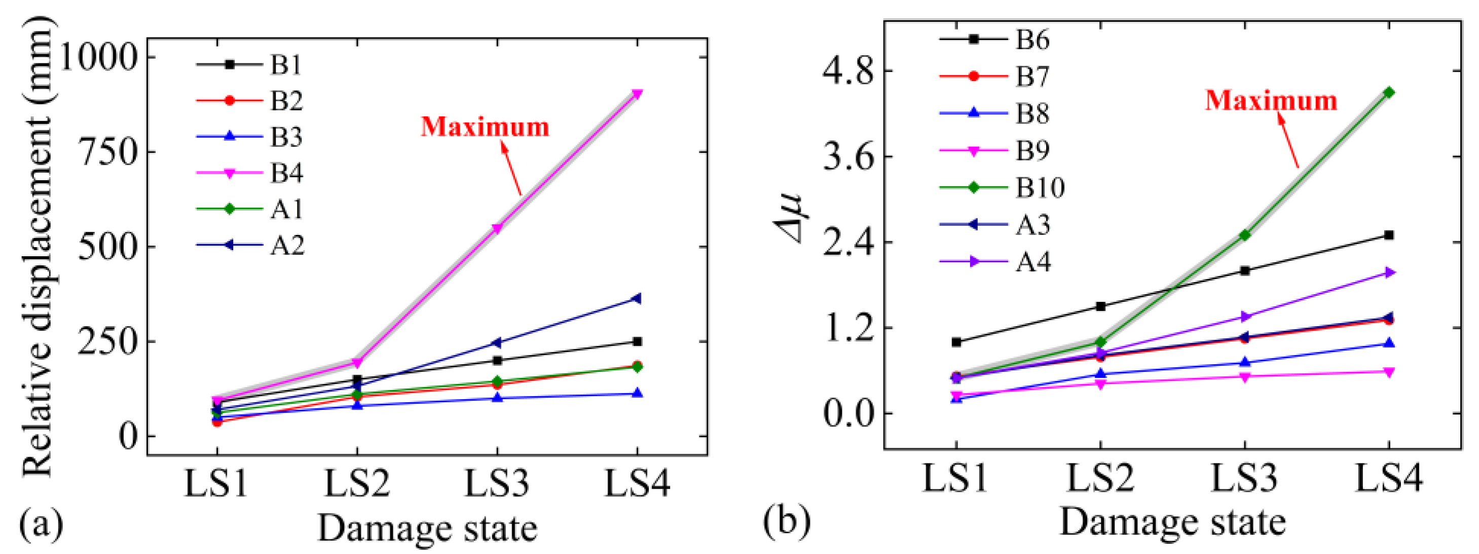
Type		LS1	LS2	LS3	LS4
Relative displacement (mm)	B1 [22]	90.00	150.00	200.00	250.00
	B2 [3]	37.40	104.20	136.10	186.60
	B3 [20]	50.00	80.00	100.00	112.50
	A1	62.50	111.40	145.40	183.00
	B4 [21]	95.00	195.00	550.00	905.00
	A2	70.60	132.30	246.50	363.50
Shear strain (%)	B5 [4]	100.00	150.00	200.00	250.00
Relative displacement ductility ratio	B6 [22]	1.00	1.50	2.00	2.50
	B7 [22]	0.52	0.79	1.05	1.31
	B8 [22]	0.20	0.55	0.71	0.98
	B9 [20]	0.26	0.42	0.52	0.59
	A3	0.50	0.82	1.07	1.35
	B10 [21]	0.50	1.00	2.50	4.50
	A4	0.50	0.85	1.36	1.98

LS1–4 represent minor damage, medium damage, serious damage, and complete destruction, respectively.

and Figure 3, based on the relative displacement, the damage indexes obtained by the empirical methods (B1–B3) have the same trend, and the values are relatively close. To save space, the damage index for the relative displacement based on empirical methods can be represented by the average value (A1) of the above three methods selected here. Similarly, the damage index using the relative displacement ductility ratio also shows this phenomenon, so A3 is selected to represent the relative displacement ductility ratio using the empirical method.

Furthermore, the damage index using the empirical method is evidently smaller than that based on the theoretical method. Especially in the serious damage and complete destruction states, the Δx obtained by the theoretical method (B4) is approximately 3.8 and 5 times that obtained by the empirical method (A1), respectively. Additionally, the Δμ obtained by the theoretical method (B10) for the above two states is approximately 2.3 and 3.3 times that obtained by the empirical method (A3), respectively. Even the indexes obtained by the empirical method are evidently less than the average values obtained by the theoretical and empirical methods. To compare the impacts of the two methods on the earthquake resistance for bearings throughout the operational lifespan, the following cases were selected in the subsequent study. See

Table 5. Case division of damage indexes for bearing.

Relative Displacement			Shear Strain	Relative Displacement Ductility Ratio
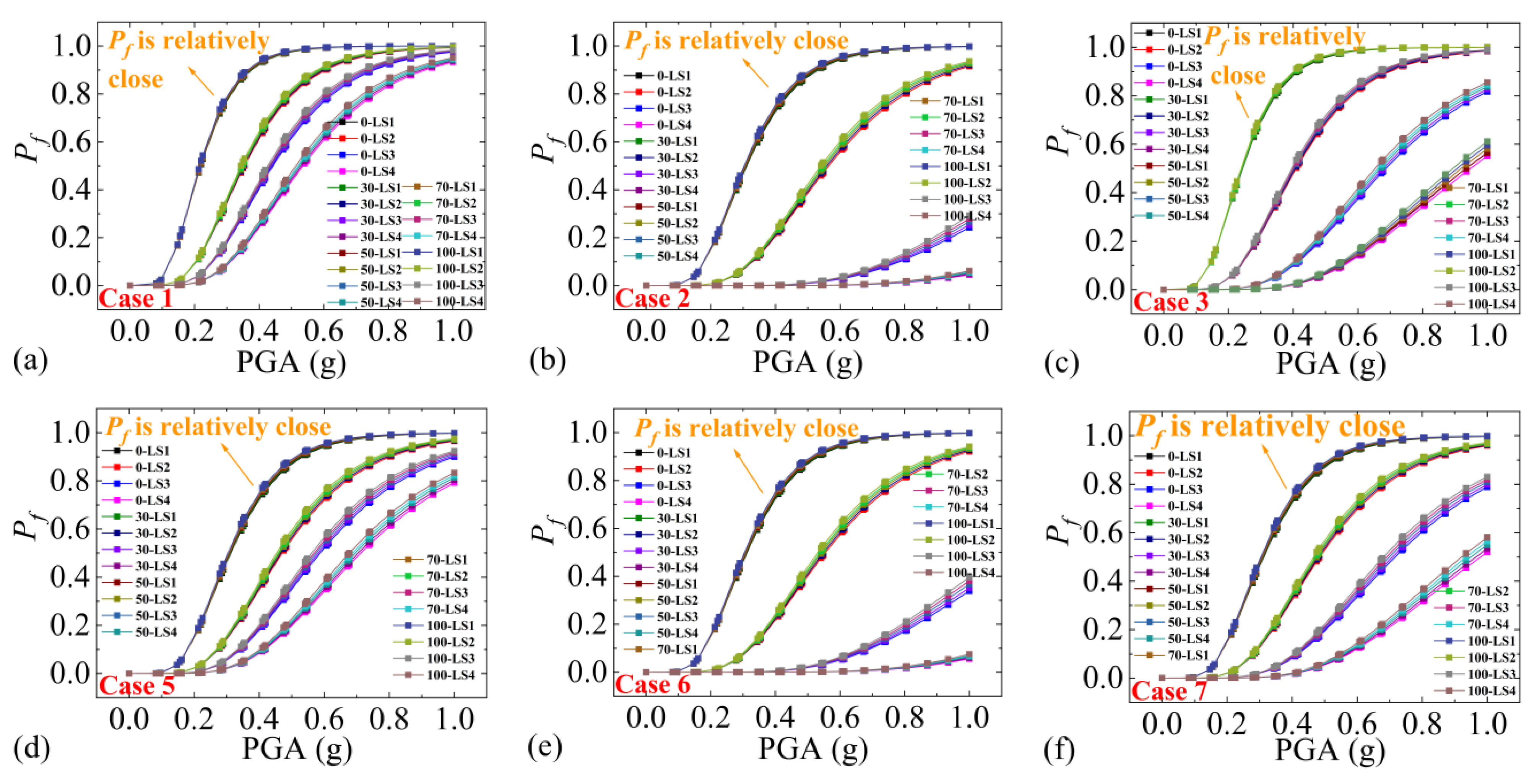
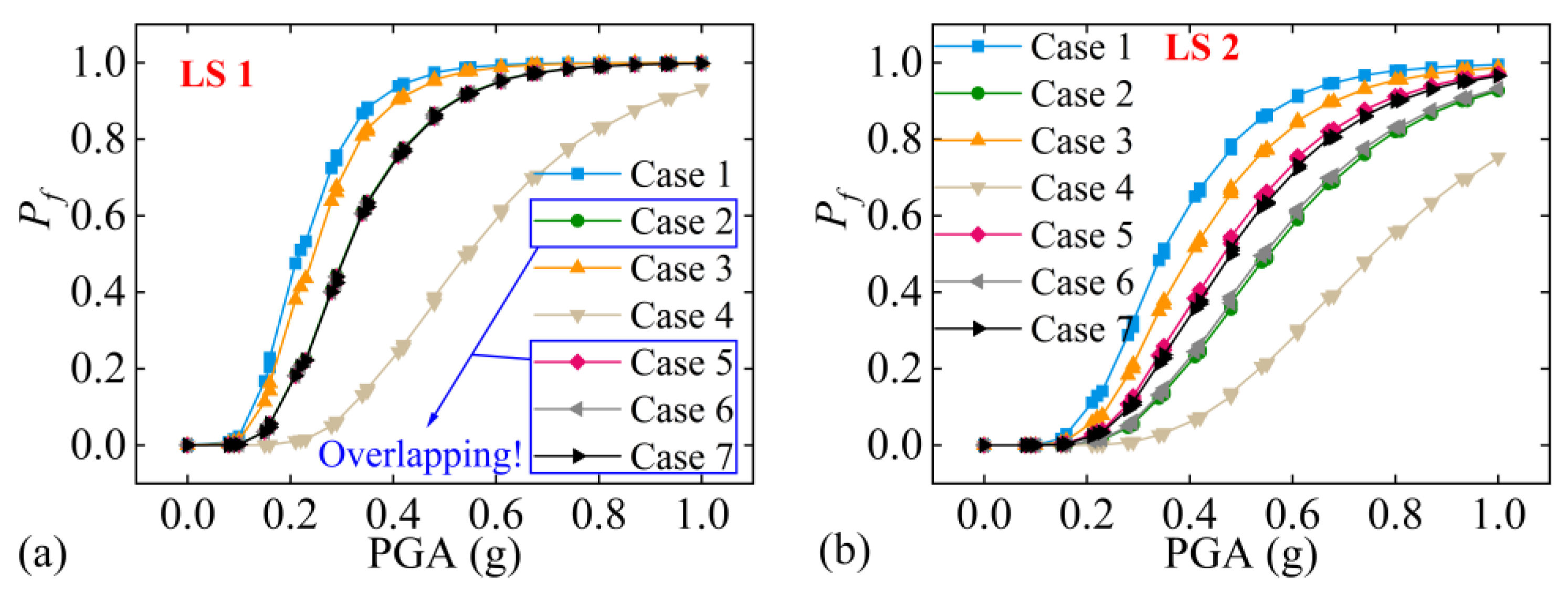
Case 1	Case 2	Case 3	Case 4	Case 5	Case 6	Case 7
A1	B4	A2	B5	A3	B10	A4

for details.

2.4. Fragility Analysis Method for Bearing

Fragility analysis involves examining the correlation between the probability of structural damage caused by seismic events and the intensity of ground motions during an earthquake. Common methods for structural seismic fragility analyses include: (1) Fragility analysis based on expert opinion: This method uses the judgment of experts to estimate the damage probability of a structure. This method has high levels of uncertainty. (2) Empirical fragility analysis method based on existing seismic damage analyses: This method uses data from past earthquakes to estimate the damage probability of a structure. This method is only applicable when using data from similar sources, and subjective differences in data collection can occur. Furthermore, many areas lack actual ground motion records. (3) Theoretical fragility analysis method based on numerical analysis: This method uses finite element analysis to simulate the behavior of a structure under earthquake loading. This method can comprehensively consider corresponding seismic records and accurately evaluate the seismic performance of structures under earthquakes. (4) Mixed fragility analysis methods: These methods combine two or more of the above three methods [1,15]. Quantitative methods based on expert opinion have high levels of uncertainty. Empirical fragility analysis methods are only applicable when using data from similar sources, and subjective differences in data collection can occur. Furthermore, many areas lack actual ground motion records. In contrast, theoretical fragility analysis methods based on finite element analysis can comprehensively consider corresponding seismic records and accurately evaluate the seismic performance of structures subject to seismic actions. Meanwhile, Liang, Yan [10] conducted analyses on the service performance of bridges using the theoretical fragility method, thereby providing further evidence of the accuracy and feasibility of this approach.

Consequently, the fragility analysis method, which relies on nonlinear dynamic time–history analysis of structures, became a crucial tool in the realm of performance-based seismic engineering. It enables a comprehensive assessment of structural performance by considering the complex nonlinear behavior of the system under seismic forces [2], as shown in Equation (17).

$$P_f=P[D\ge \left.C\right|IM]$$

(17)

where P_f is the conditional probability of damage. D is the seismic demand of the structure under random earthquake action. C is the structural response under earthquakes, corresponding to its bearing capacity. IM is the ground motion intensity. In the subsequent analysis, the earthquake resistance for the bridge will be evaluated using theoretical fragility as indicated by Equation (18).

$$P_f[D\ge C\left|IM\right.]=\Phi [(\frac{-\ln ({\mu }_C/{\mu }_D)}{\sqrt{\beta }})]=\Phi [(\frac{\ln ({\mu }_D/{\mu }_C)}{\sqrt{{{\beta }_D}^2+{{\beta }_C}^2}})]$$

(18)

where Φ (∙) refers to the standard normal cumulative distribution function, μ_C and β_C represent the mean and logarithmic standard deviation of the seismic capacity of the structure, respectively, while μ_D and β_D represent the mean and logarithmic standard deviation of the seismic demand placed on the structure, respectively [23].

Based on the properties of regression, ln (μ_D/μ_C) is assumed to follow a normal distribution of the peak ground acceleration [2,6,24,25]. Additionally, according to 100 example bridges and 100 ground motion records, Hwang, Liu [2] found that D and IM were linearly correlated on a logarithmic scale representation. See Equation (19) for details.

$$\ln ({\mu }_D)=\ln a+b\cdot \ln (IM)$$

(19)

where the coefficients a and b are determined through regression analysis.

The failure probability can be updated to the following equation:

$$P_f[D\ge C\left|IM\right.]=\Phi [(\frac{-\ln ({\mu }_C/{\mu }_D)}{\sqrt{{{\beta }_D}^2+{{\beta }_C}^2}})]=\Phi [(\frac{\ln (a\cdot I{M}^b/{\mu }_C)}{\sqrt{{{\beta }_D}^2+{{\beta }_C}^2}})]$$

(20)

where μ_C can be represented by the damage index value of the component under different damage states. Following the recommendations in HAZUS99, the value of the parameter “$\sqrt{{{\beta }_D}^2+{{\beta }_C}^2}$” is set at 0.4 for SA and at 0.5 for PGA.

3. Problem Definition

3.1. Detailed Numerical Model of the Bridge Structure

An offshore bridge is taken as the example. The girder section has an equal height, a single box, and a chamber (C50 concrete). Piers 1#, 4#, and 5# are piers with bearings (C40 concrete); piers 2# and 3# are rigid frame piers (C50 concrete); the bridge piers are all constructed as solid diamond-shaped piers. For more details on the material properties of concrete, please refer to Table 2. The longitudinal reinforcement and stirrup are made of HRB 335 and R235 reinforcement, respectively, with diameters of 32 mm and 16 mm, respectively. The thicknesses of the protective layers for the two are 103 mm and 90 mm, respectively. For more details on the material properties of longitudinal reinforcement and stirrup, please refer to Table 3. The bearings are spherical movable steel bearings. The address environment of the example bridge is a fortified area with a basic earthquake intensity of 7 degrees, located in a class II site, with good foundation conditions, mostly weakly weathered rock and slightly weathered rock, with relatively high stiffness. The detailed structure of the bridge is shown in Figure 4 [10,17].

As for the superstructure, the bridge structure is primarily prone to damage at the piers and bearings under earthquakes. Unless the bridge girder collapses, it does not undergo plastic deformation, and the dynamic response of the superstructure under earthquakes is primarily characterized by elastic deformation. Therefore, it is assumed that the superstructure behaves as an elastic component [9,26]. All loads borne by the superstructure are equivalent to the nodal masses acting on the girder.

In the concept of ductility design, the accuracy of the computational modeling of bridge piers is vital [19]. The Open System for Earthquake Engineering Simulation (OpenSees) provides two types of elements for simulating the nonlinear mechanical behavior of components: (1) The displacement-based “beam column element” (i.e., fiber elements based on the stiffness method) can be obtained through the three-time hermit difference. However, this method cannot well reflect the curvature distribution at the end of the element after yielding, and the calculation convergence speed is slow. (2) The force-based “beam column element” (i.e., fiber elements based on the flexibility method) only needs to be obtained by linear difference, which is more conducive to the simulation of curved beam–column elements, and the calculation convergence speed is faster. Thus, the nonlinear mechanical behavior of the piers is modeled using the “nonlinear beam column element” by the flexibility method. As for the fiber section of a pier, the Gauss–Lobatto integration algorithm mandates that the fiber section characteristics of each integration point must be consistent. Among them, the fibers of the confined concrete section are divided into 30 layers along the transverse direction and 15 layers along the longitudinal direction. The fibers of the unconstrained concrete section corresponding to the short side are divided into 1 layer along the transverse direction and 15 layers along the longitudinal direction; the fibers of the unconstrained concrete section corresponding to the long side are divided into 30 layers along the transverse direction and 1 layer along the longitudinal direction, and each longitudinal reinforcement is a fiber section. In addition, to reconstruct the plastic deformation of the ductile member (pier) under earthquakes, a plastic hinge area is set on the pier. With the “zero-length element”, the plastic hinge is set at the bottom of the 1#, 4#, and 5# piers (piers with bearings), and at the top and bottom of the 2# and 3# piers (rigid frame piers). Among them, the top of the rigid frame pier and the bottom of the girder at the same position are treated as common nodes. The connection between the top of the pier with the bearing and the bottom of the girder is realized by the bearing simulated by a “zero-length element”. See Figure 5 for details.

Regarding the bearings, spherical movable steel bearings are utilized in this study. The structural composition and types of these bearings are illustrated in Figure 4, Figure 5 and Figure 6, and detailed information can be found in

Table 6. Details of the bearings’ setup.

Number of Bearings	Type of Bearings	N (kN)	K1 (kN/m)	K2 (kN/m)	K3 (kN/m)
bearing 1#	MDMB	4410.5	44,105	44,105	6,250,000
bearing 3#	MDMB	9580.0	95,800	95,800	6,250,000
bearing 5#	MDMB	5685.0	56,850	56,850	6,250,000
bearing 2#	LMB	4410.5	1,250,000	44,105	6,250,000
bearing 4#	LMB	9580.0	1,250,000	95,800	6,250,000
bearing 6#	LMB	5685.0	1,250,000	56,850	6,250,000

K₁, K₂, and K₃ indicate the stiffness values of the bearing in the transverse, longitudinal, and vertical directions, respectively. MDMB and LMB indicate multi-directional movable bearing and longitudinal movable bearing, respectively.

. The QZ series spherical bearing is a special basin-type rubber bearing that consists of an upper bearing plate, lower bearing plate, spherical disc, polytetrafluoroethylene (PTFE) sliding plate, and rubber stopper. It is designed with a spherical PTFE plate instead of a rubber plate in traditional basin-type rubber bearings, which reduces the friction coefficient. The displacement is achieved by sliding between the upper bearing plate and the flat PTFE plate. It can be configured as a unidirectional movable bearing or a fixed bearing by incorporating guidance slots or rings on the upper bearing plate. The rotational movement of the bearing is facilitated by the sliding between the spherical disc and the spherical PTFE plate. In the numerical analysis, as the spherical bearing has nonlinear characteristics, an “elastic-perfectly plastic material” is used to define its stiffness in each direction, and a “zero-length element” is used to simulate the bearing. For piers with bearings, each pier is equipped with two bearings, which are multi-directional sliding bearings and longitudinal sliding bearings.

According to Li, Wu [22] and Wu, Li [1], the relative sliding between PTFE sliding plates and stainless steel plates in the movable pot bearing and movable spherical bearing allows for nearly complete relative displacement. Thus, a hysteresis model of PTFE sliding bearings is adopted to simplify the computational modeling. Test results from all types of PTFE slide bearings show that the dynamic hysteresis curve has a similar stress–strain relationship to that of an ideal elastic–perfectly plastic material. In summary, the hysteretic model shown in Figure 6 is adopted, and the calculation of the three-dimensional stiffness of the bearings is shown in Equations (21) and (22).

$$K\cdot x_y=F$$

(21)

$$\mu \cdot N=F$$

(22)

where K is the horizontal shear stiffness (kN/m), x_y is the critical sliding displacement (0.002 m), F is the sliding friction force (N), μ is the friction coefficient (0.02), and N is the load of the superstructure borne by the bearing (N). The horizontal stiffness of the multi-directional movable bearings and the longitudinal stiffness of the longitudinal movable bearings are calculated based on the actual vertical force borne by each bearing. The vertical stiffness of both types of bearings and the transverse stiffness of longitudinal movable bearings are calculated using the maximum bearing capacity of the bearings. Specifically, the maximum bearing capacity of the longitudinal movable bearings in the transverse direction is assumed to be 20% of its vertical bearing capacity (12,500 kN), as shown in Table 6. In summary, the nonlinear numerical model for the example bridge in this study was established by OpenSees, as shown in Figure 4, Figure 5 and Figure 6. In the numerical model, it is assumed that the vertical stiffness of the bearing is completely rigid, and the vertical displacement of the bearing can be constrained by a large stiffness. The vertical stiffness (K₃) of the bearings is assumed to be 5 times that of K₁, providing a strong constraint.

3.2. Ground Motion Input

The seismic motion refers to the shaking of the ground in the vicinity of Earth’s surface resulting from the propagation of seismic waves originating from an earthquake source. The key contributors to earthquakes that play a decisive role in structural damage are the ground motion intensity, spectral characteristics, and duration of strong earthquakes [27]. Currently, seismic motions can be categorized into two main groups: artificial ground motions and actual ground motions. In the seismic analysis of bridges, suitable seismic records can be chosen based on the response spectra derived from the spectral characteristics of the earthquake motion. However, the response spectrum given in seismic codes is generally obtained by taking an average value after the calculation and classification of the actual ground motion and ignoring the randomness of the actual ground motion [28]. Thus, in this study, the ground motion records were obtained based on the Pacific Earthquake Engineering Research Center (PEER). As a key factor in a seismic fragility analysis, seismic intensity is vital in seismic fragility analysis and is essential for calculating theoretical fragility. Ghosh and Padgett [11] conducted an evaluation of various measures of seismic intensity with regard to efficiency, practicality, sufficiency, and the ability to calculate hazard, and found that PGA is a highly sufficient IM for conditioning fragility analysis. Meanwhile, a probability distribution for the PGA can be obtained using current seismic records [29,30,31]. Moreover, Zhang [31] and Liang, Yan [9] demonstrated that increasing the number of selected seismic records to a sufficient quantity (over 20) can effectively mitigate the dispersion of PGA.

In summary, the following details were determined: (1) The chosen seismic motion should possess a consistent PGA including the maximum amplitudes of both common and infrequent earthquakes at the bridge location. (2) The average velocity of a shear wave in accordance with the site classification should be used to ensure that the response spectrum of the chosen seismic records closely matches the actual response spectrum. (3) The duration of the earthquake motion should ideally range from 5 to 10 times the fundamental period of the bridge to ensure that the bridge piers receive an adequate amount of seismic energy. (4) A minimum epicentral distance of greater than 20 km should be met to ensure the exclusion of the influence from near-field seismic records [17]. For this study, PGA was chosen as the ground motion intensity, and 10 suitable earthquakes were chosen from the PEER data [1,9]. By adjusting the amplitude, 10 sets of 150 seismic records were generated, as presented in

Table 7. Information from 10 original seismic records.

No.	Name	Event	Time (Year)	Site	PGA (g)	Magnitude (M)
1	RSN-138	Tabas, Iran	1978	Boshrooyeh	0.24	7.35
2	RSN-164	Imperial Valley-06	1979	Cerro Prieto	0.37	6.53
3	RSN-286	Irpinia, Italy-01	1980	Bisaccia	0.25	6.90
4	RSN-776	Loma Prieta	1989	Hollister-South and Pine	0.32	6.93
5	RSN-827	Cape Mendocino	1992	Fortuna-Fortuna Blvd	0.22	7.01
6	RSN-880	Landers	1992	Mission Creek Fault	0.31	7.28
7	RSN-1008	Northridge-01	1994	LA-W 15th St	0.32	6.69
8	RSN-1100	Kobe, Japan	1995	Abeno	0.31	6.90
9	RSN-4840	Chuetsu-oki, Japan	2007	Joetsu Kita	0.30	6.80
10	RSN-6886	Darfield, New Zealand	2010	Canterbury Aero Club	0.35	7.00

and Figure 7.

4. Results and Discussion

4.1. Incremental Dynamic Analysis

Incremental dynamic analysis (IDA) is a technique of performing a range of nonlinear time-domain dynamic evaluations of a structure by varying the magnitude of one (or more) seismic records [30]. At this time, the curve connecting the increasing IM with the corresponding structural response is called the “IDA curve”. Currently, three typical methods are commonly used for IDA: (1) Equal step method: he IM is increased in equal steps. The step size should be different for different structures. (2) Variable step method: The step size may be larger or smaller for a certain seismic record. The differences in the IM of curves approaching a horizontal line make the analysis steps required for each IDA curve different. The step value can be increased or decreased based on the convergence of the calculations. (3) Hunt and fill method: This method is based on the variable step method. An IM value is selected from the IM interval corresponding to the maximum convergence and minimum non-convergence for analysis until the interval is less than the allowable value. After that, the median value of the two IM values with the largest interval is taken for analysis until the maximum convergent IM interval is less than the allowable value [29,32]. In this study, the equal step method was selected to improve the calculation efficiency [9]. A single IDA curve can fully reflect the entire process of a structure from elasticity to failure with increasing ground motion intensity. Figure 8 shows that as the PGA increases, the IDA curves of the relative displacement of the bearings do not exhibit an evident yield platform. The slope of the curves changes slightly and can be approximately regarded as a straight line.

Further, IDA curves for bearings 1#–6# subject to the Cape Mendocino ground motion (Figure 9) during their entire life cycles are also studied (Figure 10). When the service life is 100 years, the maximum relative displacements of bearings 1#–6# under the Cape Mendocino ground motion are 0.68 m, 0.68 m, 0.69 m, 0.69 m, 0.71 m, and 0.71 m, respectively. The relative displacements of the bearings above the same pier are basically the same, and the relative displacements of bearings 5# and 6# are the largest. Therefore, as representatives, the bearings 1#, 3#, and 5# were selected for comparative analysis of the IDA curves under PGA ≥ 0.5 g, with bearings in service for 0 years, 50 years, and 100 years serving as examples. Figure 10g indicates that the IDA curves of bearings 1# and 3# on piers 1# and 4# are basically the same in the service period, which is slightly lower than the IDA curve of bearing 5# located at the pier 5#. This observation can be explained by the fact that the heights of piers 1# and 4# are comparable, whereas pier 5# is about 1.7 times taller than the former two. In terms of a given cross-section, a pier with greater height possesses relatively greater flexibility. Additionally, piers 1# and 4# are adjacent to rigid frame piers, resulting in a greater restraint effect than pier 5#. In general, the IDA curves of each bearing exhibit basically similar characteristics. For instance, the region bounded by the curve and the PGA axis is almost consistent across the different bearings. While the relative displacements of bearings on different piers may vary during their service periods, the maximum difference does not exceed 1.5%. Therefore, it is reasonable to assume that the IDA curves of bearings 1#–6# exhibit similar behavior.

To further analyze the relationship between the classification of damage states and PGA under different algorithms, bearing 5# with a larger relative displacement was selected as an example after 50 years of bridge service and subjected to the Cape Mendocino ground motion.

Table 8. Correlation between damage state classification and PGA.

Damage State	Type	No Damage	LS 1	LS 2	LS 3	LS 4
Case 1	Empirical method	PGA ≤ 0.14	0.14 < PGA ≤ 0.20	0.20 < PGA ≤ 0.25	0.25 < P GA ≤ 0.32	PGA > 0.32
Case 2	Theoretical method	PGA ≤ 0.18	0.18 < PGA ≤ 0.34	0.34 < PGA ≤ 0.84	PGA > 0.84	-
Case 3	Mean value	PGA ≤ 0.15	0.15 < PGA ≤ 0.23	0.23 < PGA ≤ 0.44	0.44 < PGA ≤ 0.64	PGA > 0.64
Case 4	Empirical method	PGA ≤ 0.33	0.33 < PGA ≤ 0.52	0.52 < PGA ≤ 0.66	0.66 < PGA ≤ 0.78	PGA > 0.78
Case 5		PGA ≤ 0.18	0.18 < PGA ≤ 0.27	0.27 < PGA ≤ 0.35	0.35 < PGA ≤ 0.48	PGA > 0.48
Case 6	Theoretical method	PGA ≤ 0.18	0.18 < PGA ≤ 0.33	0.33 < PGA ≤ 0.78	PGA > 0.78	-
Case 7	Mean value	PGA ≤ 0.18	0.18 < PGA ≤ 0.28	0.28 < PGA ≤ 0.48	0.48 < PGA ≤ 0.66	PGA > 0.66

shows the results of the analysis.

Table 8 shows that the coverage ranges of PGA for the shear strain, relative displacement ductility ratio, and relative displacement obtained based on the theoretical method are greater than those using the empirical method in the service period. As an example, if the relative displacement is adopted as the criterion, the coverage of PGA associated with minor damage for the theoretical method (Case 2) is about 267% of that for the empirical method (Case 1), and the latter (Case 1) is 75% of the average value (Case 3) of the two. If the relative displacement ductility ratio is adopted as the criterion, the coverage for the theoretical method (Case 6) is about 167% of that for the empirical method (Case 5), and the latter is about 90% of the average value (Case 7) of the two.

Additionally, compared with the relative displacement, the PGA values corresponding to the different damage states using the relative displacement ductility ratio are larger. After 50 years of service for the bearing, the PGA values for Case 7 are 121% (minor damage), 120% (medium damage), 108% (serious damage), and 103% (complete destruction) compared to those of Case 3, respectively. That is, when the damage degree for bearing is small, the difference between them is as high as 20%, whereas when the damage degree increases, the gap between the two is small, at approximately 5%. Since the quantification method of the damage index based on the relative displacement ductility ratio incorporates the principle of shear strain, Case 4 will not be specifically discussed here. In summary, the selection of different damage indexes significantly affects the assessment of the bearing’s damage state throughout the operational lifespan. The analysis framework is presented in Figure 11.

4.2. Comparison of Various Damage Indexes for Bearings

We further analyze the characteristics and applicability of the theoretical and empirical method, as well as the impacts of various damage indexes on the performance for bearings throughout the operational lifespan. As representatives, the bearings 1#, 3#, and 5# were selected for comparative analysis of the regression fitting curves for the seismic response, with bearings in service for 0 years as examples. As depicted in Figure 12, a strong linear correlation can be observed between the dynamic response of bearings and PGA. The fitting curves for bearings 1# and 3# are almost identical and are noticeably smaller than the fitting curve for bearing 5#, thus reinforcing the previous observation.

Subsequently, a time-dependent fragility analysis was conducted on bearing 5# using different damage indexes throughout the service period, as depicted in Figure 13, Figure 14 and Figure 15.

The probabilities of exceeding the threshold for the bearings in all six cases increase as the service life extends. Throughout the service period, the time-dependent deterioration of materials has a negligible effect on the probabilities subject to minor and medium damage states. However, as the damage worsens, the probabilities show a significant increase as the service period prolongs. Considering the example of the area enclosed by the fragility curve and PGA-axis after 50 years of service, it can be observed that the increase in probabilities is minimal for low damage degrees (minor and medium damage), with an increment of approximately 1%. In contrast, for higher damage degrees, the change in the probabilities is more significant, with an increase of up to 7%.

Take the increment for the probabilities subject to minor and serious damage during the service period of 0–50 years as an example (Figure 14 and Figure 15). Focusing on the relative displacement, when the degree of damage degree is small and large, the maximum increment for the probabilities obtained by the theoretical method is 168%, and 143% is obtained by the empirical method, respectively. Furthermore, when the relative displacement ductility ratio is considered, the difference in the maximum increment obtained by the theoretical and empirical methods can be ignored when the extent of damage is low. When the extent of damage is significant, the maximum increment of the probabilities using the theoretical method is larger, at approximately 129% of that using the empirical method. Furthermore, when the damage is minor, the maximum increment of the probabilities using the relative displacement ductility ratio (Case 7) is approximately 147% of that obtained by the relative displacement (Case 3), whereas the value is approximately 105% when the damage degree is large. As the damage severity increases, the maximum increment of the exceedance probability shifts towards a higher PGA value. For minor damage, the maximum increment is observed near a PGA of 0.5 g, while for more severe damage, it occurs near a PGA of 0.9 g. It is evident that as the damage severity of the bearing increases, it becomes more sensitive to strong ground motion.

Moreover, to further examine the relation between the general cost of the structure and the probability of failure, the overall expenditure is partitioned into construction costs and failure maintenance costs [33]. The construction expenses are considered to be constant, while the failure maintenance cost is determined as the multiplication of the cost of upkeep and the failure probability of the structure. See Equation (23) for details.

$$C_B{=C}_c+C_{fm}\cdot P_f$$

(23)

where P_f is the probability of failure for the structure, C_B, C_c, and C_fm are the overall expenditure, construction expenses, and cost of upkeep, respectively. In simpler terms, the exceedance probability plays a crucial role in determining the balance between the economy and safety of the structure’s seismic design. In summary, if security is more important, a damage index calculation method with a higher increment of exceedance probability should be selected, while, if the economy is the focus, the damage index calculation method with a smaller increment of exceedance probability should be selected. See

Table 9. Application of damage index (by the increment of exceedance probability).

Type	When the Extent of Damage Is Low (LS1 and LS2)	When the Extent of Damage Is Significant (LS3 and LS4)
Security	Case 5, Case 6, and Case 7	Case 2 and Case 6
Economy	Case 1	Case 1 and Case 5

for more details.

Although the exceedance probability of the bearing exhibits the characteristic of continuous increase with the prolongation of service time, the increment is relatively small. Merely examining the change rate of the failure probabilities throughout the operational lifespan of the structure is insufficient for assessing the suitability of the damage index. Figure 16 illustrates the comparison of time-varying fragility for different cases, using bearing 5# as an example after 50 years of service. This analysis aims to further enhance the applicability of various damage indexes.

Figure 16 demonstrates a positive correlation between the failure probabilities of the bearing and the PGA. Throughout the operational lifespan of the structure, the exceedance probability for the bearing using the relative displacement is greater than that using the relative displacement ductility ratio, and the difference between them increases with an increase in the damage degree. As an example, the enclosed region between the curve and the PGA-axis calculated by the relative displacement (Case 1) are approximately 120%, 128%, 131%, and 151% larger than those using the relative displacement ductility ratio (Case 5) for the four damage states, respectively.

Focusing on relative displacement, irrespective of the extent of damage, the exceedance probability derived from the empirical method (Case 1) is always greater than that obtained based on the theoretical method (Case 2). Moreover, the failure probability calculated using the theoretical method (Case 2) is even lower compared to the probability obtained by averaging the results of the two methods (Case 3). When the extent of damage is low (minor damage), specifically considering the relative displacement ductility ratio, the probability obtained by empirical and theoretical methods is basically equal. When the damage is slightly aggravated (medium damage), it shows the same trend as the relative displacement, and the probability obtained by the empirical method (Case 5) is greater. When the damage degree continues to increase, the exceedance probability obtained by the empirical method (Case 5) is also greater, but the probability obtained by the average value (Case 7) of empirical and theoretical methods is closer to that obtained by the empirical method.

Table 10. Application of damage indexes (based on the order of exceedance probability).

Type	LS1	LS2	LS3	LS4
Security	Case 1
Economy	Case 3		Case 5

presents the discussion for the damage indexes using the ranking of the fragility curves throughout the operational lifespan of the bridge.

Table 9 and Table 10 reveal that the classification of the damage indexes for bearings based on the order of the exceedance probability and that from the ranking order of its increment are different. That is, the magnitude of the exceedance probability of the bearing itself is not related to its increment throughout the operational lifespan. Additionally, the probability for the bearing obtained using the relative displacement is larger, and its increment during the service period is smaller. On the contrary, the probabilities for the bearings obtained using the relative displacement ductility ratio are relatively small, but their increments during the service period are significant.

This phenomenon can be attributed to the fact that piers, especially high piers, have more prominent bending deformation under earthquakes. In a similar scenario, the concept of performance-based ductility design is incorporated by considering the relative displacement ductility ratio, which accounts for the shear deformation of the piers. As a result, the relative displacement ductility ratio-based index for each damage state tends to be higher, resulting in a lower probability of exceeding. By exclusively focusing on relative displacement without considering shear deformation, the resulting indexes for damage states tend to be small. Consequently, this leads to a higher failure probability. In conclusion, Table 10, based on the order of exceedance probability, is more suitable for the division of the damaged state of bearings subject to earthquakes.

5. Summary and Conclusions

In this study, numerical analysis was conducted on an offshore bridge to investigate the comparison of damage indexes for assessing the seismic fragility of bearings in an offshore bridge. The study yielded the following conclusions:

(1) The damage index using the theoretical method is notably larger compared to the one obtained through the empirical method. For example, in terms of the coverage of PGA under minor damage, when using relative displacement as the chosen index, the coverage obtained by the theoretical method is 267% greater than that obtained by the empirical method. Moreover, when using the relative displacement ductility ratio to determine the damage indexes for the four damage states, the corresponding PGA is higher compared to when using relative displacement as the damage index.

(2) As the service life extends, the failure probabilities for the bearings under various damage indexes tend to increase. The impact of time-dependent effects on the exceedance probability is minimal and subject to minor and medium damage states. As the degree of damage increases, there is a substantial increase in the failure probability with the prolongation of the operational lifespan. Following a service period of 50 years, the exceedance probability for the complete destruction state increases by 7% compared to 0 years of service. Additionally, the sensitivity of the bearing to strong earthquakes also increases with the damage degree. As the level of damage increases, the probability calculated using relative displacement outweighs that calculated using the relative displacement ductility ratio, and the disparity between them amplifies during the service period.

(3) The relative displacement ductility ratio, which incorporates the shear deformation of the piers, is a preferable option, as it aligns more effectively with the concept of performance-based ductility design and offers cost advantages. In regions prone to seismic activity, it is advisable to employ a damage index focused on safety for evaluating the earthquake resistance for the bearings. However, in less severe environments, an index emphasizing economic factors may be more suitable.

References

- Wu, W.P.; Li, L.F.; Shao, X.D. Seismic Assessment of Medium-Span Concrete Cable-Stayed Bridges Using the Component and System Fragility Functions. J. Bridge Eng. 2016, 21, 04016027. [Google Scholar] [CrossRef]
- Hwang, H.; Liu, J.; Chiu, Y. Seismic Fragility Analysis of Highway Bridges; The University of Memphis: Memphis, TN, USA, 2001. [Google Scholar]
- Nielson, B. Analytical Fragility Curves for Highway Bridges in Moderate Seismic Zones; Georgia Institute of Technology: Atlanta, GA, USA, 2005. [Google Scholar]
- Zhang, J.; Huo, Y.L. Evaluating effectiveness and optimum design of isolation devices for highway bridges using the fragility function method. Eng. Struct. 2009, 31, 1648–1660. [Google Scholar] [CrossRef]
- Alam, M.S.; Bhuiyan, M.; Billah, A. Seismic fragility assessment of SMA-bar restrained multi-span continuous highway bridge isolated by different laminated rubber bearings in medium to strong seismic risk zones. Bull. Earthq. Eng. 2012, 10, 1885–1909. [Google Scholar] [CrossRef]
- Shinozuka, M.; Feng, M.Q.; Kim, H.K.; Kim, S.H. Nonlinear static procedure for fragility curve development. J. Eng. Mech. 2000, 126, 1287–1295. [Google Scholar] [CrossRef] [Green Version]
- Parool, N.; Rai, D.C. Seismic Fragility of Multispan Simply Supported Bridge with Drop Spans and Steel Bearings. J. Bridge Eng. 2014, 20, 04015021. [Google Scholar] [CrossRef]
- Taskari, O.; Sextos, A. Multi-angle, multi-damage fragility curves for seismic assessment of bridges. Earthq. Eng. Struct. Dyn. 2015, 44, 2281–2301. [Google Scholar] [CrossRef]
- Liang, Y.; Yan, J.L.; Cheng, Z.Q.; Chen, P.; Ren, C. Time-varying seismic fragility analysis of offshore bridges with continuous rigid-frame girder under main aftershock sequences. J. Bridge Eng. 2020, 25, 04020055. [Google Scholar] [CrossRef]
- Liang, Y.; Yan, J.L.; Qian, W.X.; Cheng, Z.Q.; Chen, H. Analysis of collapse resistance of offshore rigid frame—Continuous girder bridge based on time-varying fragility. Mar. Struct. 2021, 75, 102844. [Google Scholar] [CrossRef]
- Ghosh, J.; Padgett, J.E. Aging Considerations in the Development of Time-Dependent Seismic Fragility Curves. J. Struct. Eng. 2010, 136, 1497–1511. [Google Scholar] [CrossRef]
- Shekhar, S.; Ghosh, J. Seismic Fragility of Highway Bridges Considering Improved Bearing Deterioration Modeling. In Maintenance, Safety, Risk, Management and Life-Cycle Performance of Bridges; CRC Press: Boca Raton, FL, USA, 2018. [Google Scholar]
- Cornell, C.A. Engineering seismic risk analysis. Bull. Seismol. Soc. Am. 1968, 58, 1583–1606. [Google Scholar] [CrossRef]
- Qian, J.; Cheng, L.; Zhou, D. Behavior of axially loaded concrete columns confined with ordinary hoops. J. Tsinghua Univ. 2002, 42, 1369–1373. [Google Scholar]
- Wu, W.; Li, L.; Shao, X.; Hu, S. Seismic evaluation of the aged high-pier and long-span bridges subjected to extremely halobiotic condition. In Proceedings of the 7th International Conference, Bridge Maintenance, Safety and Management, Shanghai, China, 7–11 July 2014; pp. 2031–2037. [Google Scholar]
- Sung, Y.C.; Su, C.K. Time-dependent seismic fragility curves on optimal retrofitting of neutralised reinforced concrete bridges. Struct. Infrastruct. Eng. 2011, 7, 797–805. [Google Scholar] [CrossRef]
- Yan, J.L.; Liang, Y.; Zhao, B.Y.; Qian, W.X.; Chen, H. Influence of time-varying attenuation effect of damage index on seismic fragility of bridge. Earthq. Struct. 2020, 19, 287–301. [Google Scholar] [CrossRef]
- Zhao, J.; Sritharan, S. Modeling of Strain Penetration Effects in Fiber-Based Analysis of Reinforced Concrete Structures Concrete Structures. ACI Struct. J. 2007, 104, 133–141. [Google Scholar]
- Mazzoni, S.; McKenna, F.; Scott, M.H.; Fenves, G.L. OpenSees command language manual. Pac. Earthq. Eng. Res. (PEER) Cent. 2006, 264, 137–158. [Google Scholar]
- Jiao, C.Y. Seismic Vulnerability Analysis of Long Span Stayed-Cable Bridge Based on Performance; Tongji University: Shanghai, China, 2008. [Google Scholar]
- Xu, D.L. Seismic Vulnerability Analysis of High Pier Continuous Rigid Bridge under the Influence of Hydrodynamic Pressure; Southwest Jiaotong University: Chengdu, China, 2018. [Google Scholar]
- Li, L.F.; Wu, W.P.; Hu, S.C.; Liu, S.M. Time-dependent seismic fragility analysis of high pier bridge based on chloride ion induced corrosion. Eng. Mech. 2016, 33, 171–178. [Google Scholar]
- Kircher, C.A.; Whitman, R.V.; Holmes, W.T. HAZUS earthquake loss estimation methods. Nat. Hazards. Rev. 2006, 7, 45–59. [Google Scholar] [CrossRef]
- Choi, E.; Desroches, R.; Nielson, B. Seismic fragility of typical bridges in moderate seismic zones. KSCE J. Civ. Eng. 2004, 26, 187–199. [Google Scholar] [CrossRef]
- Shome, N.; Cornell, C.A.; Bazzurro, P. Earthquakes, Records, and Nonlinear Responses. Heart Rhythm Off. J. Heart Rhythm Soc. 2012, 6, 85. [Google Scholar] [CrossRef]
- Zhang, J.H. Study on Seismic Vulnerability Analysis of Normal Beam Bridge Piers Based on Numerical Simulation; Tongji University: Shanghai, China, 2006. [Google Scholar]
- Ye, A.J. Seismic Design of Bridges; China Communications Press: Beijing, China, 2017. [Google Scholar]
- Song, Y.T.; Zhu, J.C. Artificially generate earthquake records compatible with code design spectrum and structural responses. J. Build. Struct. 1983, 3, 43–54. [Google Scholar]
- Bertero, V.V. Strength and deformation capacities of buildings under extreme environments. Struct. Eng. Struct. Mech. 1977, 53, 211–215. [Google Scholar]
- Vamvatsikos, D.; Cornell, C. Incremental dynamic analysis. Earthq. Eng. Struct. Dyn. 2002, 31, 491–514. [Google Scholar] [CrossRef]
- Zhang, H.Y. Displacement-Based Probabilistic Seismic Demand Analysis and Structure Seismic Design Research; Hunan University: Changsha, China, 2000. [Google Scholar]
- Wang, M.P.; Cao, X.J.; Sun, W.L. Incremental dynamic analysis applied to seismic risk assessment of hybrid structure. Earthq. Resist. Eng. Retrofit. 2010, 32, 109–121. [Google Scholar]
- Yan, J.L.; Guo, A.X.; Li, H. Comparative analysis of different types of damage indexes of coastal bridges based on time-varying seismic fragility. Mar. Struct. 2022, 86, 103288. [Google Scholar] [CrossRef]