
An Assessment Scheme for Road Network Capacity under Demand Uncertainty


Abstract
1. Introduction
2. Network Capacity Problem under Demand Uncertainty
2.1. The Uncertainty of Network Capacity
2.2. Travel Demand Uncertainty Analysis
2.3. Road Network Capacity Model with Uncertain Demand
- Network capacity is represented by a uniformly increased or decreased multiplier; therefore, the reserve capacity model is straightforward to solve.
- Given that the initial/current O–D matrix is regarded as an uncertain parameter in the reserve capacity model, the demand distribution is no longer fixed but variable within a given range.
3. Sensitivity-Analysis-Based Approximation Method
- The solution to the network capacity problem for a given nominal O–D demand;
- Perturbation analysis of the travel demand ;
- The linear approximation of the reaction function.
3.1. Solving the Capacity Model with Nominal Demand
| Algorithm 1: Solving the capacity model with the nominal O–D demand. |
| Step 0: Initialization. Determine the initial values of the O–D demand, . and initial value . Set n: = 0. Step 1: Solving the PSL model. Solve the PSL model based on , and obtain the equilibrium solution . Step 2: Sensitivity analysis. Use the sensitivity analysis approach to obtain the partial derivatives () for the PSL model. Step 3: Local linear approximation. By employing the derivatives to create local linear approximations of the upper-level capacity restrictions, the approximate linear programming problem can then be solved to create an auxiliary multiplier . Step 4: Updating solution. Let , where is a predetermined step size, e.g., . Step 5: Convergence criterion. Stop if the convergence requirement has been met; if not, return to Step 1 and set n: = n + 1. |
3.2. Sensitivity Analysis under Demand Uncertainty
3.3. Linear Approximation of the Reaction Function
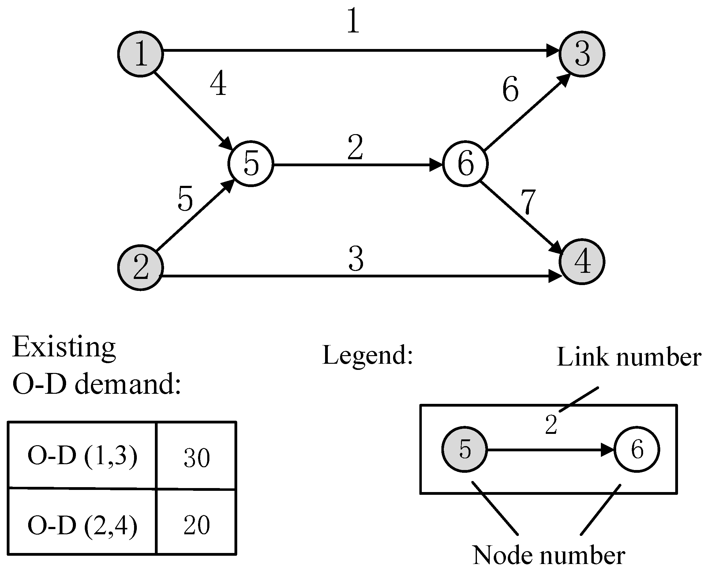
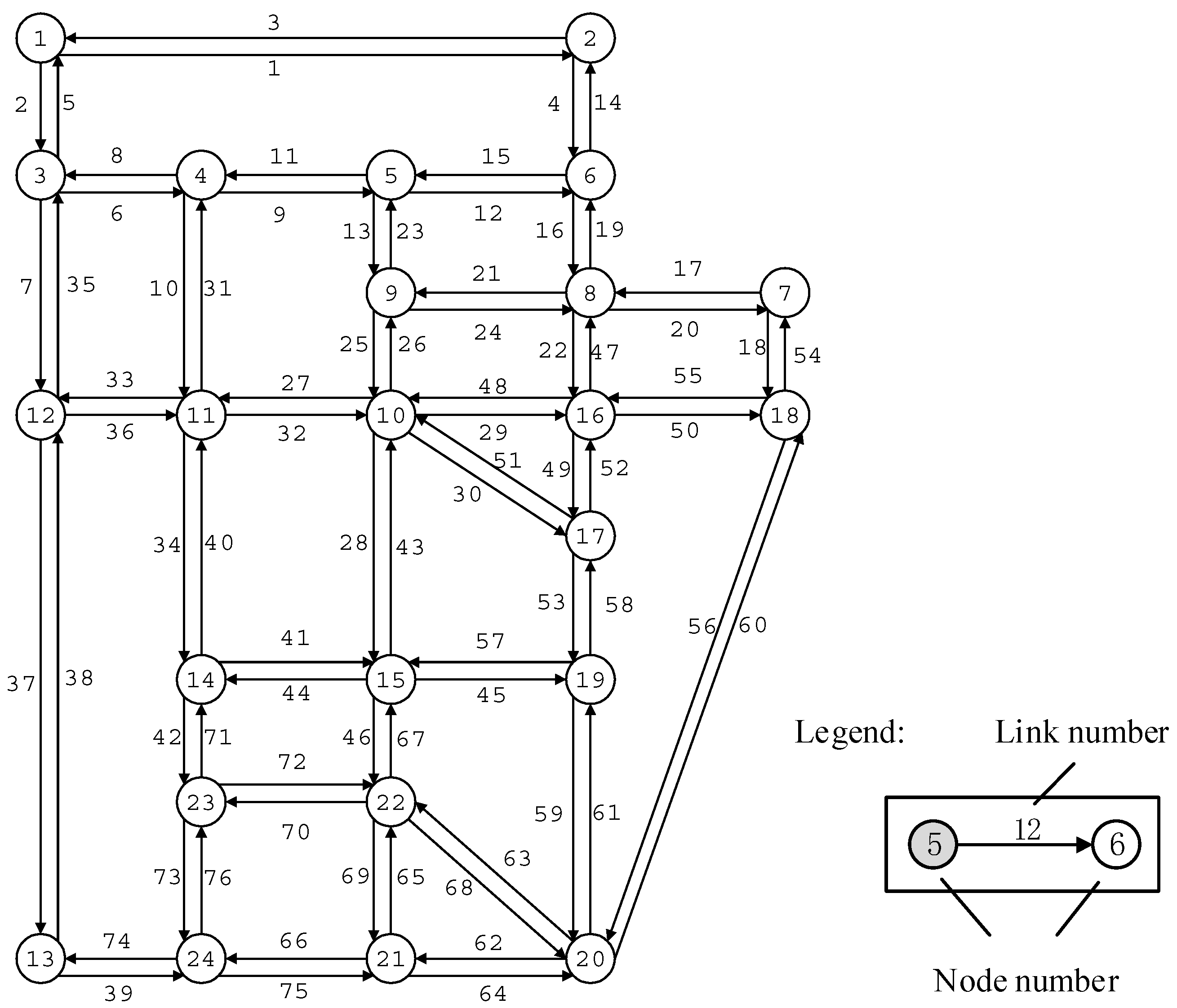
4. Numerical Experiments
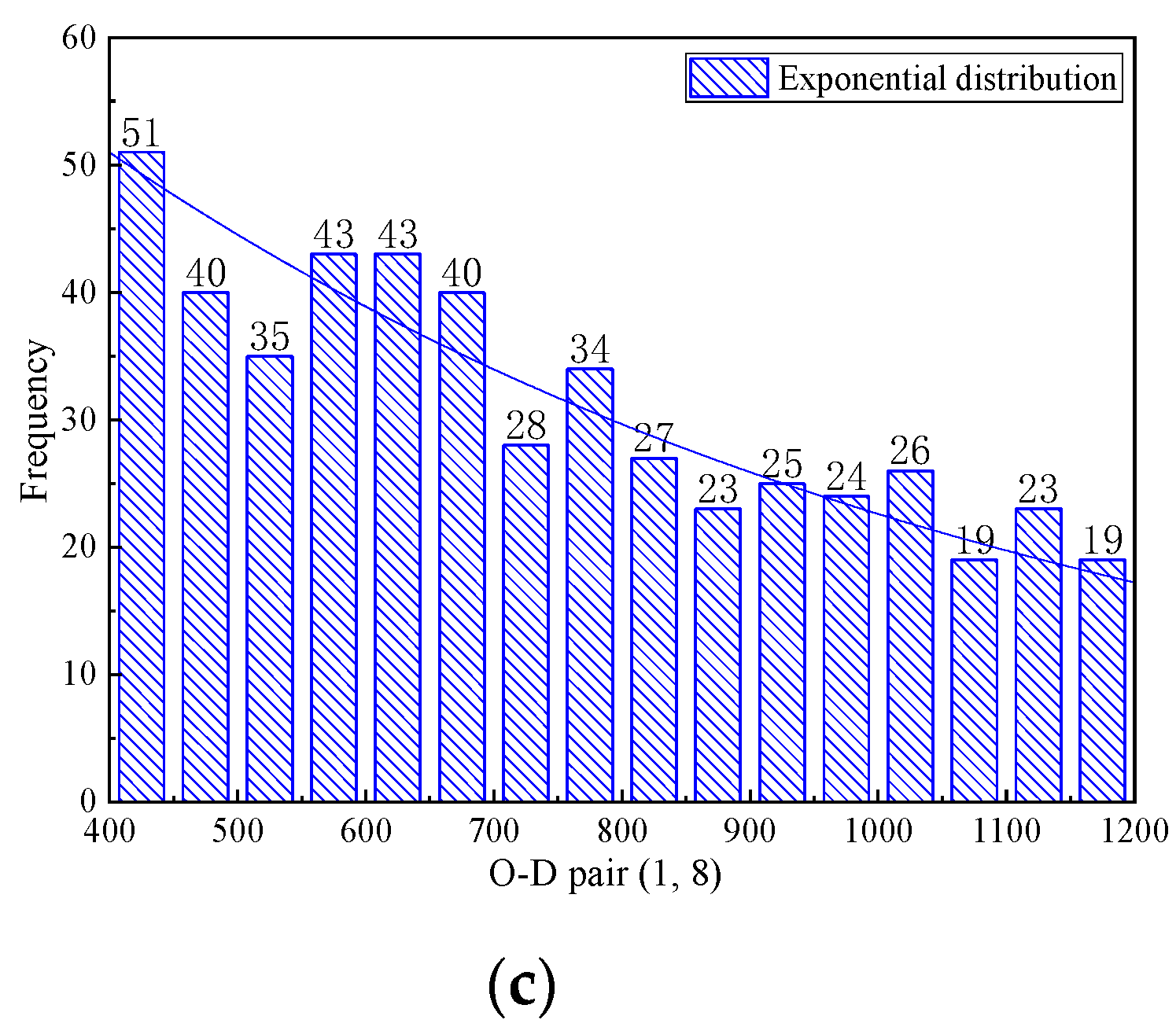
4.1. The Random Sampling Distribution of the Travel Demand
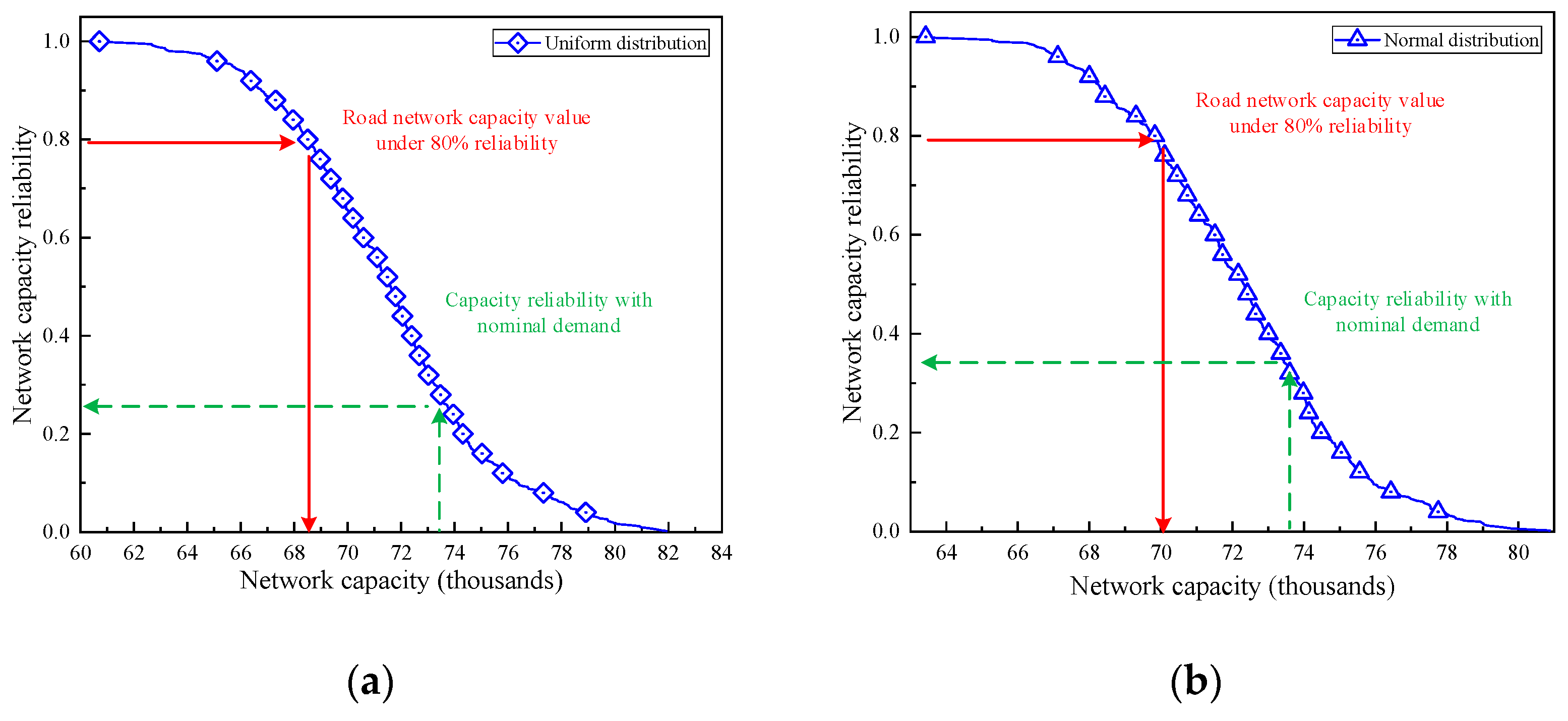
4.2. Analysis of Network Capacity Reliability
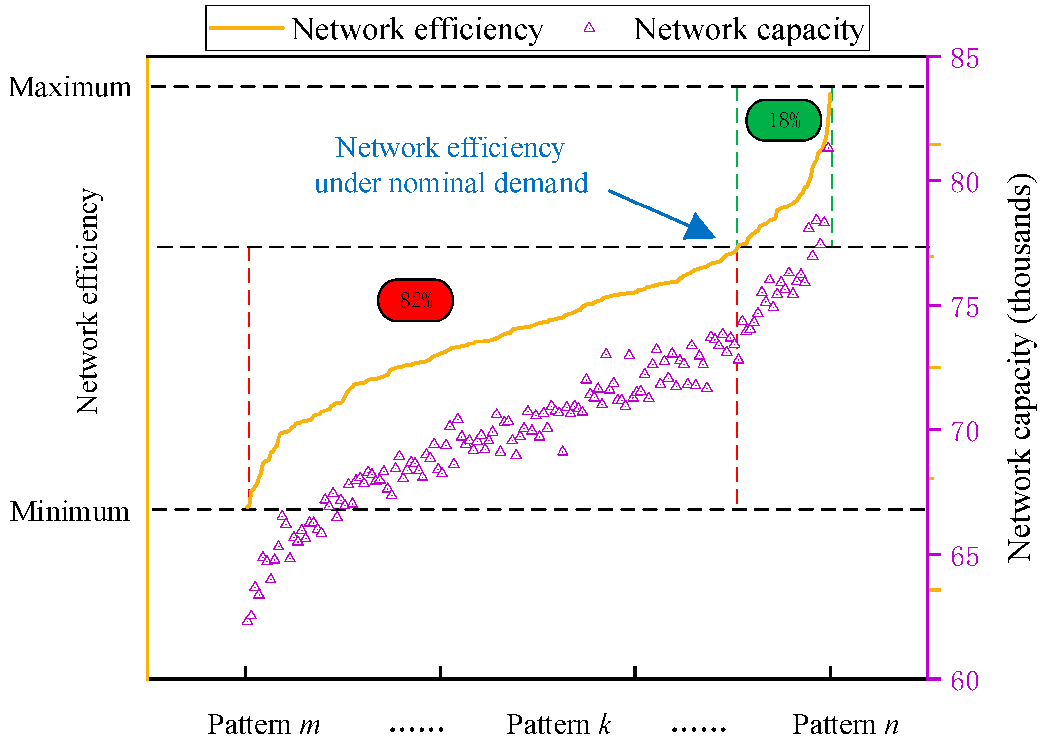
4.3. The Efficiency of Road Network
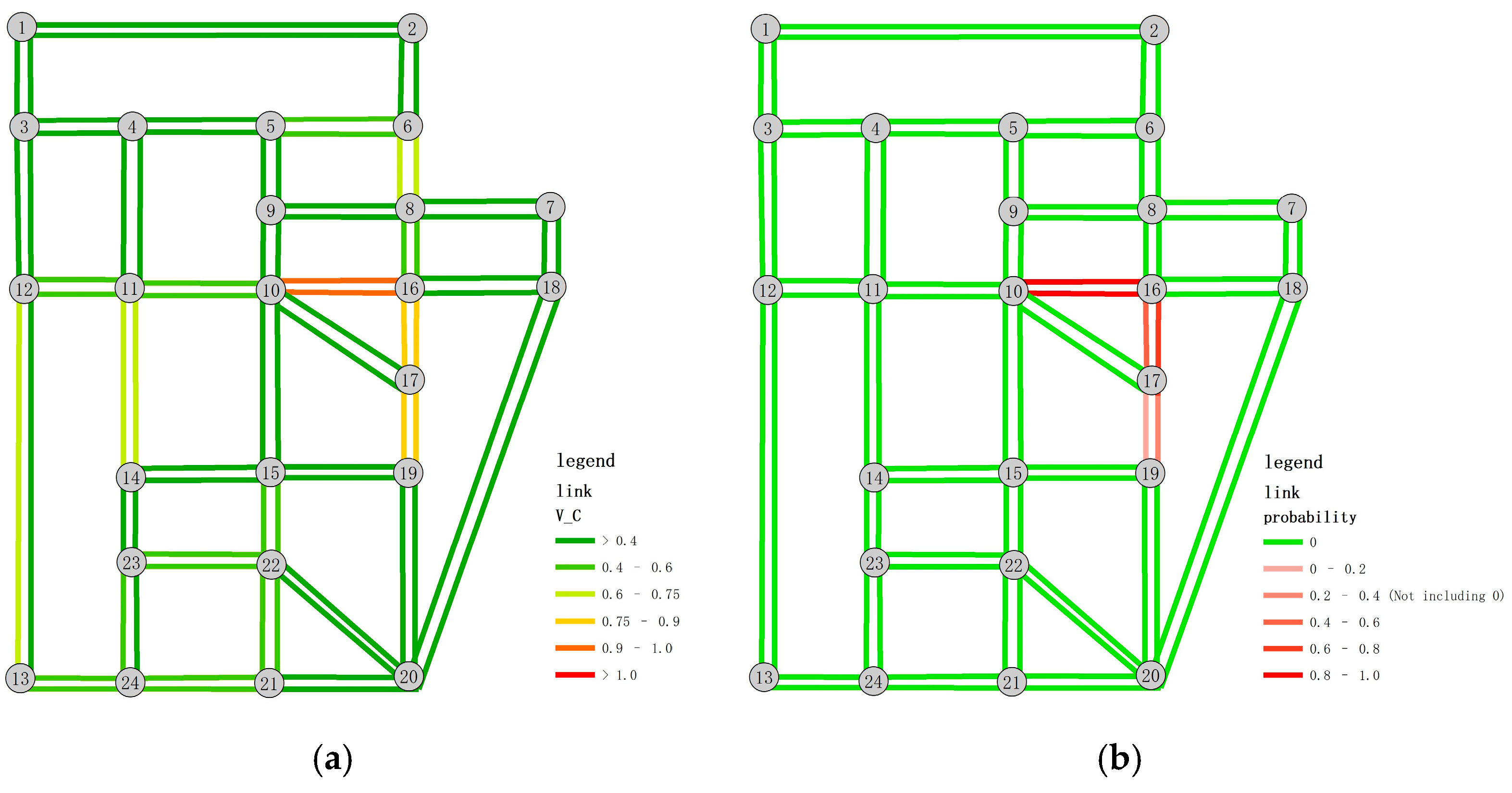
4.4. Critical Link Identification with Uncertain Demand
4.5. Critical OD Pair Identification with Uncertain Demand
4.6. Performance of the Sensitivity-Based Approximate Approach
4.6.1. Error Analysis
4.6.2. The Efficiency of SAB Algorithm
5. Conclusions
Author Contributions
Funding
Institutional Review Board Statement
Informed Consent Statement
Data Availability Statement
Conflicts of Interest
Appendix A. Sensitivity Analysis of the PSL Model
References
- Wong, S.C.; Yang, H. Reserve capacity of a signal-controlled road network. Transp. Res. Part B Methodol. 1997, 31, 397–402. [Google Scholar] [CrossRef]
- Ceylan, H.; Bell, M.G.H. Reserve capacity for a road network under optimized fixed time traffic signal control. Intell. Transp. Syst. 2004, 8, 87–99. [Google Scholar] [CrossRef]
- Chiou, S.W. Reserve capacity of signal-controlled road network. Appl. Math. Comput. 2007, 190, 1602–1611. [Google Scholar] [CrossRef]
- Xu, X.; Chen, A.; Jansuwan, S.; Yang, C.; Ryu, S. Transportation network redundancy: Complementary measures and computational methods. Transp. Res. Part B Methodol. 2018, 114, 68–85. [Google Scholar] [CrossRef]
- Zhou, J.K.; Du, M.Q.; Chen, A. Multimodal urban transportation network capacity model considering intermodal transportation. Transp. Res. Rec. 2022, 2676, 357–373. [Google Scholar] [CrossRef]
- Jiang, X.W.; Shan, X.N.; Du, M.Q. Modeling Network Capacity for Urban Multimodal Transportation Applications. J. Adv. Transp. 2022, 2022, 6034369. [Google Scholar] [CrossRef]
- Du, M.Q.; Zhou, J.K.; Chen, A.; Tan, H.Q. Modeling the capacity of multimodal and intermodal urban transportation networks that incorporate emerging travel modes. Transp. Res. Part E Logist. Transp. Rev. 2022, 168, 102937. [Google Scholar] [CrossRef]
- Kasikitwiwat, P. Capacity Reliability and Capacity Flexibility of a Transportation Network. Ph.D. Dissertation, Utah State University, Logan, Utah, 2005. [Google Scholar]
- Kasikitwiwat, P.; Chen, A. Analysis of transportation network capacity related to different system capacity concepts. J. East. Asia Soc. Transp. Stud. 2005, 6, 1439–1454. [Google Scholar]
- Tam, M.L.; Lam, W.H.K. Maximum car ownership under constraints of road capacity and parking space. Transp. Res. Part A-Policy Pract. 2000, 34, 145–170. [Google Scholar] [CrossRef]
- Chen, A.; Kasikitwiwat, P. Modeling capacity flexibility of transportation networks. Transp. Res. Part A Policy Pract. 2011, 45, 105–117. [Google Scholar] [CrossRef]
- Zheng, Y.; Zhang, X.; Liang, Z. Multimodal subsidy design for network capacity flexibility optimization. Transp. Res. Part A Policy Pract. 2020, 140, 16–35. [Google Scholar] [CrossRef]
- Liu, Z.; Wang, Z.; Cheng, Q.; Yin, R.; Wang, M. Estimation of urban network capacity with second-best constraints for multimodal transport systems. Transp. Res. Part B Methodol. 2021, 152, 276–294. [Google Scholar] [CrossRef]
- Duell, M.; Garder, L.M.; Dixit, V.; Waller, S.T. Evaluation of a strategic road pricing scheme accounting for day-tO–Day and long-term demand uncertainty. Transport. Res. Rec. 2014, 2467, 12–20. [Google Scholar] [CrossRef]
- Chen, A.; Zhou, Z. The α-reliable mean-excess traffic equilibrium model with stochastic travel times. Transport. Res. B-Meth. 2010, 44, 493–513. [Google Scholar] [CrossRef]
- Waller, S.T.; Fajardo, D.; Duell, M.; Dixit, V. Linear programming formulation for strategic dynamic traffic assignment. Netw. Spat. Econ. 2013, 13, 427–443. [Google Scholar] [CrossRef]
- An, K.; Lo, H.K. Robust transit network design with stochastic demand considering development density. Transport. Res. B-Meth. 2015, 81, 737–754. [Google Scholar] [CrossRef]
- Sun, Y.; Liang, X.; Li, X.Y.; Zhang, C. A fuzzy programming method for modeling demand uncertainty in the capacitated road-rail multimodal routing problem with time windows. Symmetry 2019, 11, 91. [Google Scholar] [CrossRef]
- Deng, Y.; Chen, X.; Yang, C. Hub-and-spoke airline network design with uncertainty demand. J. Triffic Transp. Eng. 2009, 9, 69–74. [Google Scholar]
- Li, Z.C.; Bing, X.; Fu, X.W. A hierarchical hub location model for the integrated design of urban and rural logistics networks under demand uncertainty. Ann. Oper. Res. 2023. [Google Scholar] [CrossRef]
- Hu, W.J.; Dong, J.J.; Ren, R.; Chen, Z.L. Layout Planning of Metro-based Underground Logistics System Network Considering Fuzzy Uncertainties. J. Syst. Simul. 2022, 34, 1725–1740. [Google Scholar]
- Jiang, J.H.; Zhang, D.Z.; Meng, Q.; Liu, Y.J. Regional multimodal logistics network design considering demand uncertainty and CO2 emission reduction target: A system-optimization approach. J. Clean. Prod. 2020, 248, 119304. [Google Scholar] [CrossRef]
- Du, M.Q.; Jiang, X.W.; Cheng, L.; Zheng, C.J. Robust evaluation for transportation network capacity under demand uncertainty. J. Adv. Transp. 2017, 2017, 9814909. [Google Scholar] [CrossRef]
- Yin, Y.; Lawphongpanich, S.; Lou, Y. Estimating Investment Requirement for Maintaining and Improving Highway Systems. Transp. Res. Part C Emerg. Technol. 2008, 16, 199–211. [Google Scholar] [CrossRef]
- Ben-Akiva, M.; Bierlaire, M. Discrete choice methods and their applications to short term travel decisions. In Handbook of Transportation Science; Hall, R.W., Ed.; Springer: Boston, MA, USA, 1999; pp. 5–11. [Google Scholar]
- Fiacco, A.V. Introduction to Sensitivity and Stability Analysis in Nonlinear Programming; Academic Press: New York, NY, USA, 1983. [Google Scholar]
- Du, M.Q.; Jiang, X.W.; Chen, A. Identifying critical links using network capacity-based indicator in multi-modal transportation networks. Transp. B Transp. Dyn. 2021, 10, 1126–1150. [Google Scholar] [CrossRef]
- Li, S.G. Reasonable Path Set Algorithm for Dynamic Traffic Assignment. J. Zhengzhou Univ. Eng. Sci. 2009, 30, 125–128. [Google Scholar]
- Qin, J.; He, Y.X.; Ni, L. Quantitative efficiency evaluation method for transportation networks. Sustainability 2014, 6, 8364–8378. [Google Scholar] [CrossRef]


| Link | 1 | 2 | 3 | 4 | 5 | 6 | 7 |
|---|---|---|---|---|---|---|---|
| 10 | 4 | 12 | 4 | 5 | 5 | 4 | |
| 100 | 80 | 80 | 50 | 120 | 50 | 50 |
| 80% Reliability of Network Capacity with Uncertain Demand | Network Capacity with Nominal Demand | |
|---|---|---|
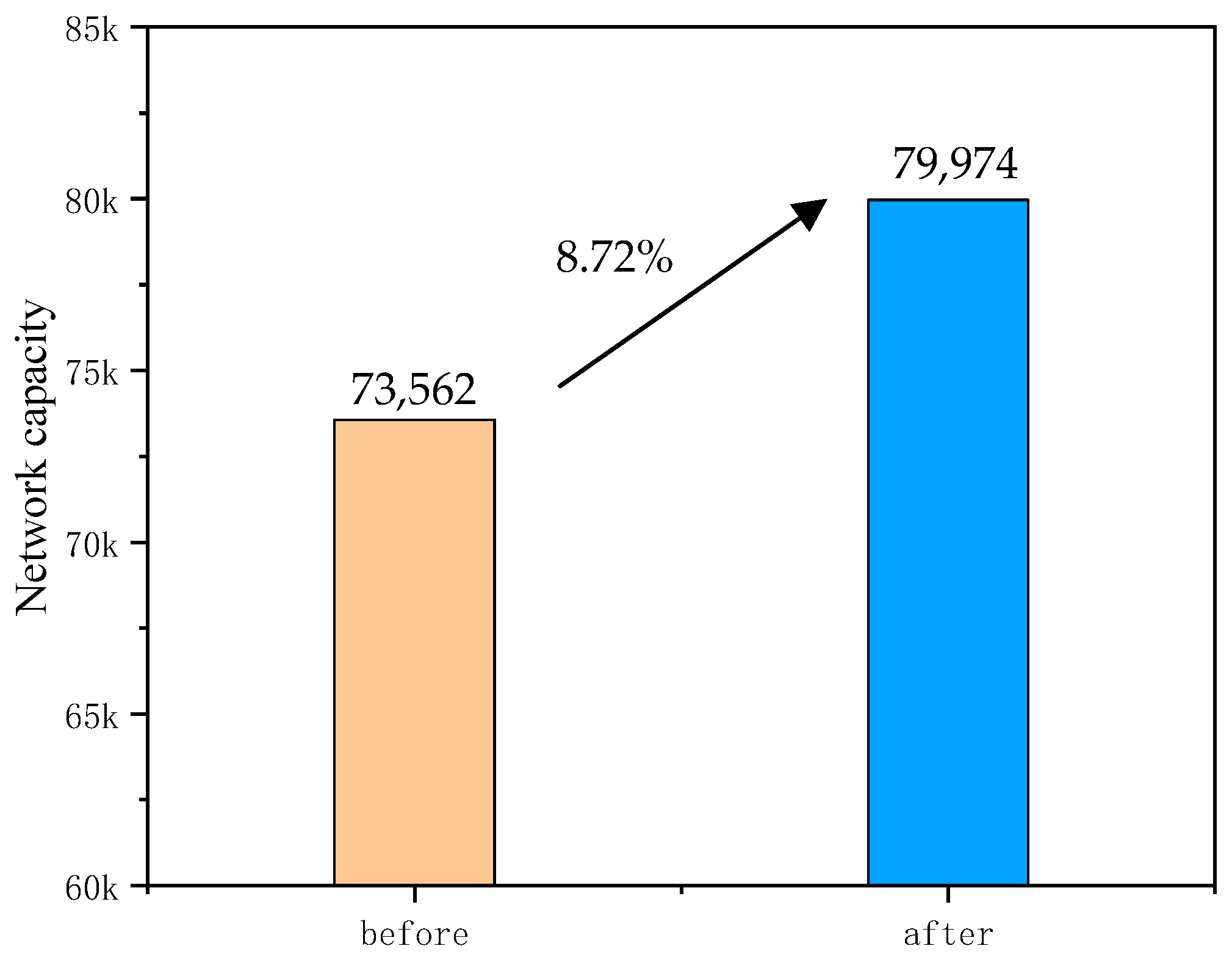
| Before improvement | 68,505 | 73,202 |
| After improvement | 84,376 | 84,020 |
| Improved ratio | 23% | 15% |
| Time (s) | Total (50 Samples) | Average |
|---|---|---|
| Exact solution approach | 5066.8 | 101.34 |
| SAB approximate approach | 114.7 | 2.29 |
Disclaimer/Publisher’s Note: The statements, opinions and data contained in all publications are solely those of the individual author(s) and contributor(s) and not of MDPI and/or the editor(s). MDPI and/or the editor(s) disclaim responsibility for any injury to people or property resulting from any ideas, methods, instructions or products referred to in the content. |
© 2023 by the authors. Licensee MDPI, Basel, Switzerland. This article is an open access article distributed under the terms and conditions of the Creative Commons Attribution (CC BY) license (https://creativecommons.org/licenses/by/4.0/).
Share and Cite
Ge, Z.; Du, M.; Zhou, J.; Jiang, X.; Shan, X.; Zhao, X. An Assessment Scheme for Road Network Capacity under Demand Uncertainty. Appl. Sci. 2023, 13, 7485. https://doi.org/10.3390/app13137485
Ge Z, Du M, Zhou J, Jiang X, Shan X, Zhao X. An Assessment Scheme for Road Network Capacity under Demand Uncertainty. Applied Sciences. 2023; 13(13):7485. https://doi.org/10.3390/app13137485
Chicago/Turabian StyleGe, Zhongzhi, Muqing Du, Jiankun Zhou, Xiaowei Jiang, Xiaonian Shan, and Xing Zhao. 2023. "An Assessment Scheme for Road Network Capacity under Demand Uncertainty" Applied Sciences 13, no. 13: 7485. https://doi.org/10.3390/app13137485
APA StyleGe, Z., Du, M., Zhou, J., Jiang, X., Shan, X., & Zhao, X. (2023). An Assessment Scheme for Road Network Capacity under Demand Uncertainty. Applied Sciences, 13(13), 7485. https://doi.org/10.3390/app13137485