Calculation Method of Loose Pressure in Surrounding Rock Mass

Abstract

With the implementation of the regional coordinated development strategy, traffic flow has grown explosively. The construction of a larger tunnel section becomes an effective way to solve the highway network’s insufficient transport capability problem. Currently, there is little research on the factors influencing and methods of calculating the loose pressure in the surrounding rock mass for highway tunnels with super-large cross-sections. Based on the Bifurcation Tunnel, which is one of the sign projects in the past five years, this paper discusses the influencing factors for the range of loose zone in deeply buried tunnels using a combination of a numerical analysis and an orthogonal test. The weight of influencing factors is calculated via an efficiency evaluation method. This paper establishes a limit analysis model of the loose pressure in the surrounding rock mass under a non-linear failure criterion based on the fitted boundary function and upper bound limit analysis method and deduces the correlations of the loose pressure. The distribution law of the loose pressure, obtained via the limit analysis method, is consistent with the pressure-monitoring results, verifying the correctness of the proposed calculation method. This study can provide a calculation basis for the design of a supporting structure and the selection of similar super-section tunnel projects.

1. Introduction

Owing to rapid economic development, logistics, and the vehicle industry, the construction of tunnels with large-span and extra-large-span sections has boomed in recent years and serves as the optimum scheme to improve road capacity and meet the existing travel demand. Compared to a single-hole project with a small span, an extra-large-span-section tunnel consists of a much larger span, a lower high-span ratio, and a greater construction risk. There are no corresponding design codes and construction standards for these projects. Although some construction experience has been obtained, theoretical research is relatively lacking.

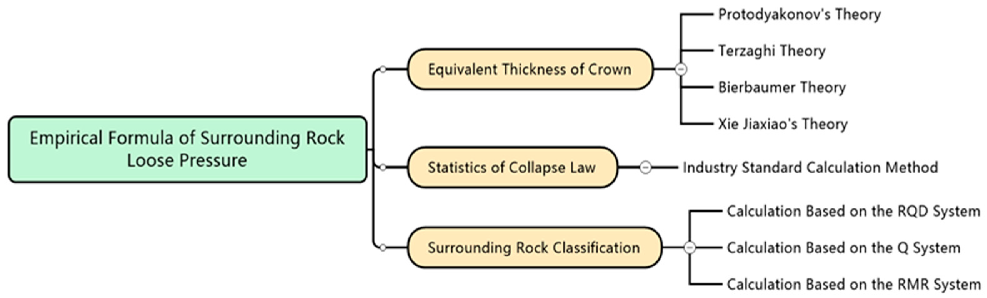
To guarantee the rationality of the supporting structure design for super-span tunnels, the first problem to be solved is to clarify the method of predicting the loose pressure in the surrounding rock mass. At present, the empirical formulas commonly used for the loose pressure are divided into three categories: the equivalent thickness of the crown, statistics of collapse law, and surrounding rock classification, as shown in Figure 1. The equivalent thickness of the crown takes the gravity of the rock and soil mass above the vault as the primary influence for the loose pressure in the surrounding rock. Typical methods include Protodyakonov’s theory [1], the Bierbaumer theory [2], the Terzaghi theory [3], and Xie Jiaxiao’s theory [4]. The statistics of collapse law method is based on practical engineering and is the leading engineering practice used in design codes in China [5,6,7,8]. The correlations are relatively simple and consider the influence of the surrounding rock classification. The surrounding rock classification method derives the surrounding rock loose pressure from the RQD, Q, and RMR systems [9,10,11,12]. The correlations and applicable conditions of various calculation methods are presented in

Table 1. Different correlations for calculation methods.

Item		Correlation	Applicable Conditions	Weakness
Protodyakonov’s theory [1]		$P=\gamma h_1$	Deep burial condition; small span	Competent coefficient of rock is determined subjectively
Terzaghi theory [3]		$P=\frac{L\gamma -2c}{2K\mathrm{t}\mathrm{a}\mathrm{n}\phi }\left[1-e^{-\frac{2K}{L}\mathrm{Htan}\phi }\right]$	Shallow burial condition; loose media	Unsuitable for rock stratum
Bierbaumer theory [2]		$P=rH\left[1-\frac{H{k}_1}{L}-\frac{2c}{L\gamma }\left(1-2k_2\right)\right]$	Shallow burial condition; loose media	Unsuitable for rock stratum
Xie Jiaxiao’s theory [4]		$P=rH\left(1-\frac{H}{B}K\mathrm{t}\mathrm{a}\mathrm{n}\theta \right)$	Shallow burial condition; small span	Unsuitable for deep burial condition
Code for the Design of Railway Tunnel (TB10003-2016) [5]		$P=\gamma h_q,h_q=0.45\times 2^{s-1}\omega$	Small span	Unsuitable for conditions with span greater than 15 m
Specification for the Design of Hydraulic Tunnels (SL279-2016) [7]		$P=\left(0.2\sim 0.3\right)\gamma B$	Specific stratum	Neglects the effect of surrounding rock conditions
Design Code of Artificial Rock Caverns (in Chinese) [8]		${P=N}_0{K}_1\gamma$	Specific stratum	Neglects the effect of surrounding rock conditions
Q System	Barton correlation [9]	$$\begin{gathered} P_1=\frac{2.0}{J_r}{Q}^{-\frac{1}{3}}\times 0.1 \\ {P}_2=\frac{2}{3}{J}_n^{\frac{1}{2}}{J}_r^{-1}{Q}^{-\frac{1}{3}} \end{gathered}$$	Small span	Neglects the effect of geometrical dimension
	Bhasin and Grimstad correlation [10]	$P=\frac{0.04B}{J_r}{Q}^{-\frac{1}{3}}$	Broken rock condition	Neglects the effect of height
RMR System	Unal correlation [11]	$P=\frac{100-RMR}{100}\gamma B$	Specific stratum	Neglects the effect of buried depth
	Goel and Jethwa correlation [12]	$P=\frac{7.5B^{0.1}{H}^{0.5}-RMR}{20RMR}$	Deep burial condition	Neglects the effect of height

Notation: γ—rock mass bulk density; $h_1$—height of natural arch; L—slip block width; c—cohesion; K—lateral pressure coefficient; ϕ—internal friction; H—tunnel height; $k_1={\tan }^2\left(45°-\varphi /2\right)$; $k_2=\tan \left(45°-\varphi /2\right)$; θ—internal friction on both sides of roof; B—tunnel width; ω—width influence coefficient; N₀—basic value of surrounding rock pressure; K₁—width correction factor; $J_n$—joint set number; $J_r$—joint roughness number.

.

There are two deficiencies of the above-mentioned empirical formulas: (1) the calculations are derived or statistically obtained under the conditions of a small-span tunnel, and (2) the influencing factors are significantly different. The above two deficiencies restrict the applications of empirical formulas for loose pressure in the extra-large-span cross-section tunnels.

In addition to the empirical formulas, the upper bound theorem of limit analysis with a strictly theoretical basis has also been used recently to calculate the loose pressure in the surrounding rock mass. It focuses on the ultimate failure state of the rock–soil mass without considering the elastic–plastic deformation process. In addition, this method is not restricted by the span. Some scholars have published papers on the surrounding rock pressure of soil tunnels. Atkinson et al. [13] discussed the stability of a shallow circular tunnel in a cohesionless soil through the upper bound theorem of limit analysis together with results of tests performed in sand soil. Davis et al. [14] deduced the upper boundary stability solutions for a shallow tunnel excavation at three different positions under undrained conditions and proposed a new stability evaluation method. In order to analyze the stability of an excavation face, Mollon et al. [15,16] established the spatial discretization three-dimensional calculation method based on the limit analysis method, and the results of the calculation approached the real situation. Based on the Hoek–Brown failure criterion, Huang et al. [17] presented an upper bound solution for the collapse shape for a circular tunnel considered the influence of different geological conditions and pore water pressure. Lei et al. [18] established explicit expressions to calculate the loose pressure on a shallow, buried tunnel based on the upper bound theorem of limit analysis and the Terzaghi failure mode. Based on the spatial discretization model, Pam et al. [19,20,21] studied the impact mechanism of a heterogeneous stratum, pore water pressure, and a non-circular excavation face on the tunnel face stability. Zhang et al. [22] proposed an analytical method for calculating the ultimate support force of an excavation face in the clay layer and analyzed the local and whole stability of the excavation face for a large-diameter shield tunnel in practical engineering. According to the tunnel face failure mode in purely cohesive soil proposed by Mollon [23], Huang et al. [24] established an analytical model considering the shear failure boundary which further improved the calculation accuracy of the upper bound solution for tunnel face stability in non-homogeneous and anisotropic undrained clay. To assess the stability of a tunnel face in inclined strata, Tu et al. [25] optimized the 3D rotating rigid body collapse mechanism by improving the spatial discretization technique. However, the failure mechanism constructed in the current research is highly subjective and lacks numerical simulation and field test verification. Such flaws can be solved by combining a numerical analysis and an upper bound limit analysis. With its lower cost, shorter period, and better repeatability, a numerical simulation is helpful for predicting the failure position [26,27]. Wang et al. [28,29] verified the rationality of the analytical solution for the collapse curve via a vertical displacement cloud picture obtained from a simulation.

In view of the shortcomings of the existing research, this paper discussed the impact of rock conditions and cavern size on the range of the loose pressure zone by combining a numerical analysis and an orthogonal test. The investigation is based on the Bifurcation Tunnel. The limit analysis model of the loose pressure in the surrounding rock is established using the fitted boundary function of the loose zone and the upper bound limit analysis. Based on this model, this paper deduces the upper bound solution for a deep tunnel’s loose pressure, which is verified by pressure-monitoring results obtained for the different sections. The results of this research can provide new ideas for the selection of a supporting structure for similar super-section tunnel projects.

2. Project Overview

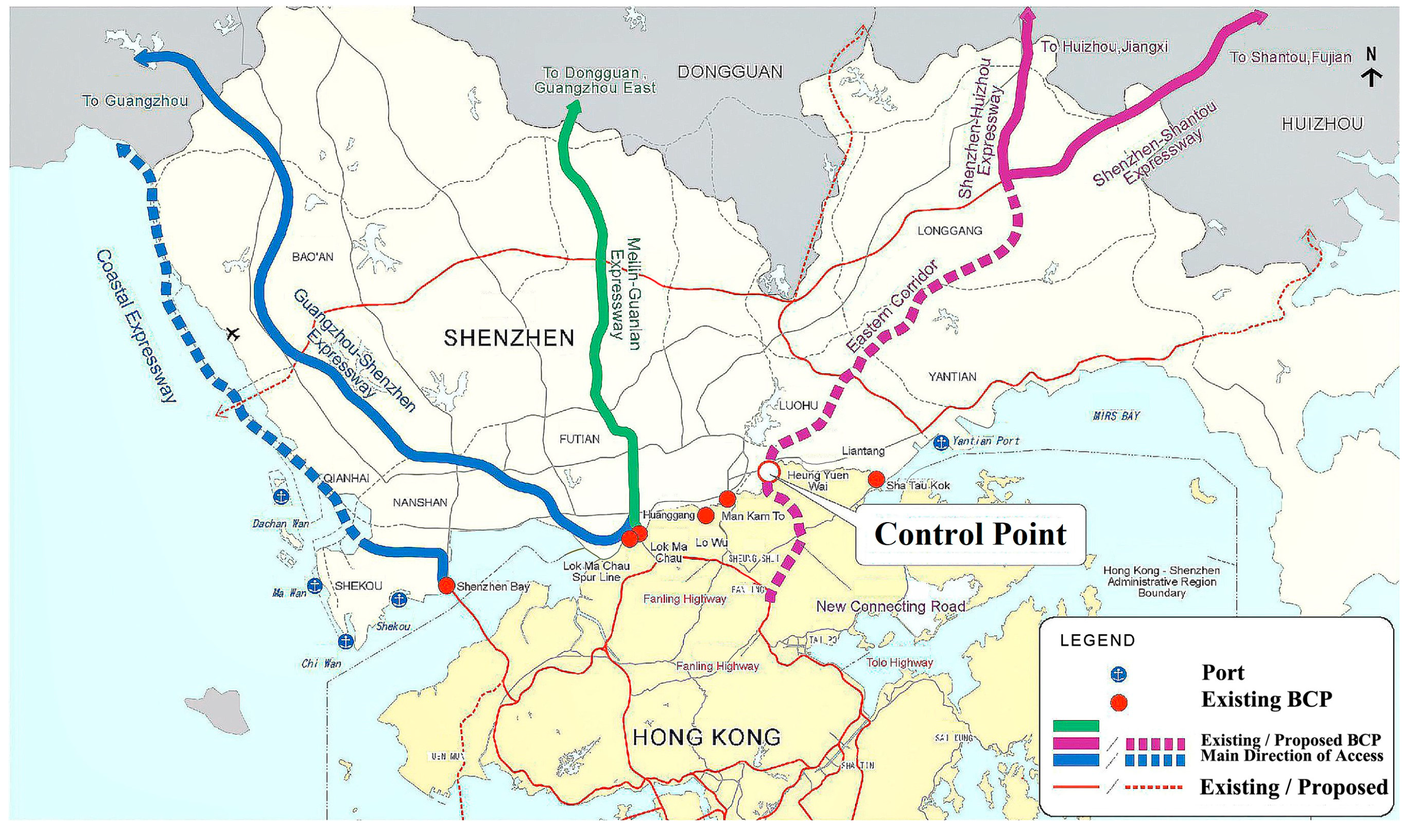
The Shenzhen Transit Expressway is a major construction project in Shenzhen, Guangdong Province, China. It begins at Luosha Road, connects with the Hong Kong highway network through the port, and ends at the Huiyan expressway. The total length of the route is 32.5 km, while the total investment is about CNY 5.792 billion. It will become a critical traffic artery serving the development of the eastern coastal areas of South China after its completion.

The eastern transit passage of Shenzhen City starts from Luohu Port, connects with the Hong Kong highway network through the port, and ends at the Huiyan expressway. The project is 32.5 km long in total, and it will become a critical traffic artery serving the development of the eastern coastal areas of South China after its completion. The passage planning is shown in Figure 2.

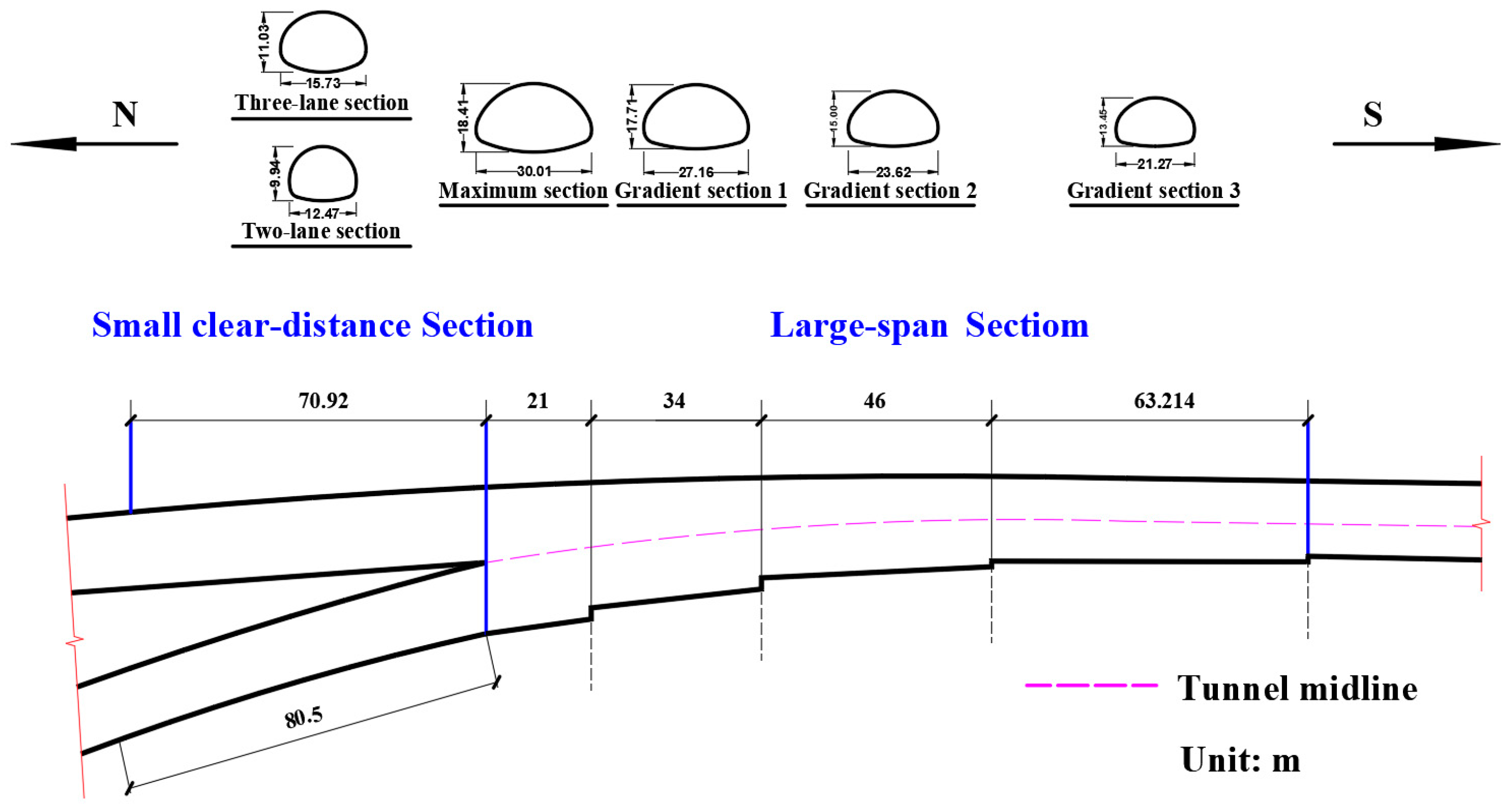
The Bifurcation Tunnel is a key control project in the entire transit expressway line and has a total length of 1435 m [30]. It is composed of three parts: the mainline section, the municipal section, and the port connecting section, of which the mainline section is divided into left and right lines. The Bifurcation Section is located at the entrance of the left line. The large-span section includes the maximum section, Gradient Section 1, Gradient Section 2, and Gradient Section 3. The Bifurcation Section is shown in Figure 3.

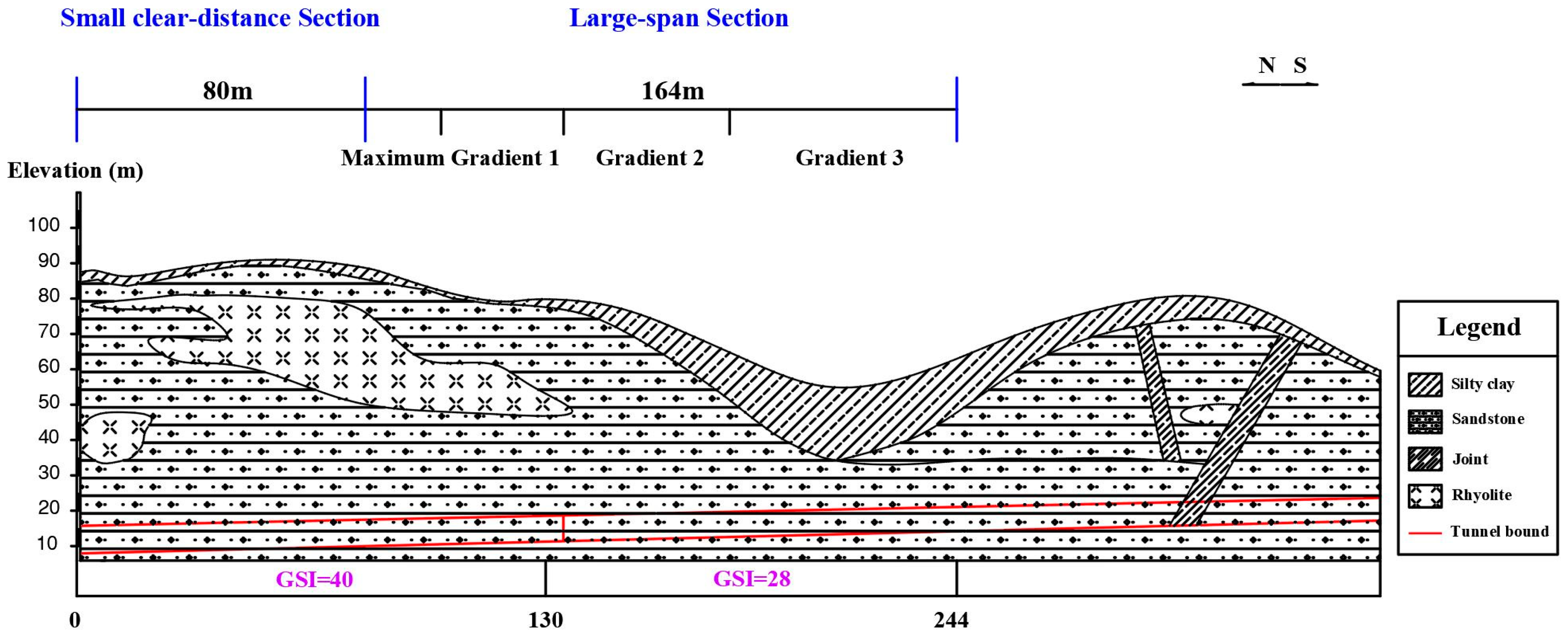
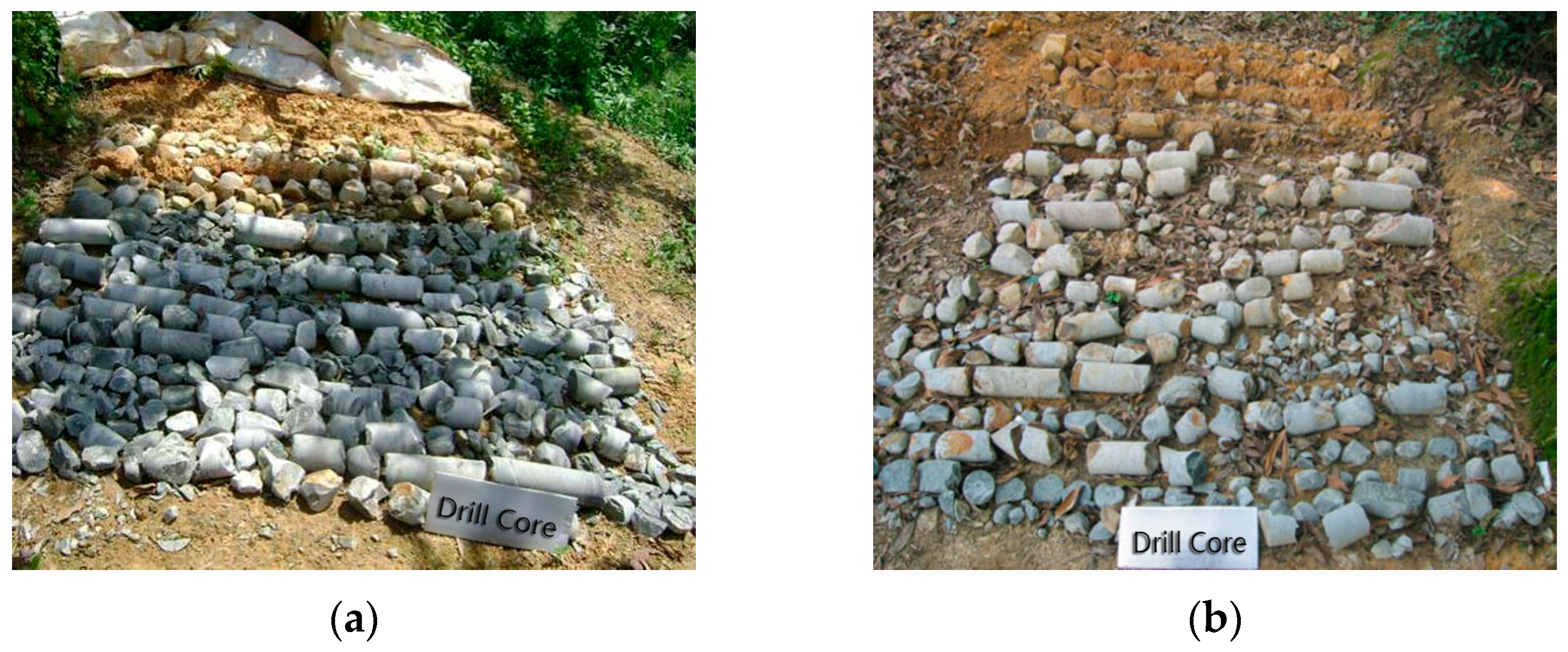
The burial depth of the large-span bifurcation section is 78~106 m. The stratum at the tunnel site consists of artificial soil, sandstone, flood alluvial soil, and rhyolite. The rock mass is relatively complete, with only slightly developed fractures to which the degree of development increases with depth. The geological section is shown in Figure 4, and photos of the drill core are shown in Figure 5. The geological investigation, combined with the rock mass type, weathering degree, and joint development, provides the GSI (geological strength index) value of the Bifurcation Section, as shown in

Table 2. Characteristics of the surrounding rock of the project.

Mileage	Length	Surrounding Rock Characteristics	GSI
0~130	130 m	The surrounding rock is slightly weathered sandstone, and the rock mass is fractured with developed joint fissures. Generally, the groundwater is poor, and the permeability is low.	40
130~244	114 m	The surrounding rock is a greenish-gray, medium, and slightly weathered sandstone. The rock mass is relatively fractured with developed joint fissures, and the rock core is short, columnar, and massive. The groundwater is poor and does not have the conditions for water inrush.	28

. Furthermore, the maximum excavation span is 30.01 m, and the maximum excavation area is 428.5 m²; globally, this is a rare extra-large section highway tunnel. Therefore, the key to the construction project’s structural design and safety is determining the influencing factors and distribution pattern of the loose pressure of the surrounding rock for the large-span section.

3. Study of Factors Influencing the Loose Zone in the Surrounding Rock Mass

The formation of the loose zone due to excavation is an inherent characteristic of the surrounding rock mass. The scope of the loose zone directly determines the loose pressure in the surrounding rock mass. Based on the orthogonal test and the finite difference software FLAC3D, this paper designs multiple group model tests to determine the influence of various factors, such as the surrounding rock quality, cavern size, and tunnel burial depth, on the loose zone of an extra-large section tunnel.

3.1. Orthogonal Analysis

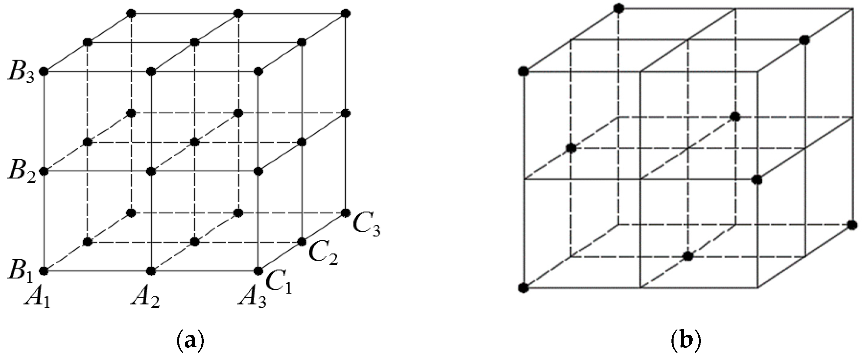
The orthogonal experimental design method, proposed by mathematical statistician R.A. Fisher in 1935, has been widely used in mathematics, economics, agriculture, aerospace, and other fields. Compared with the comprehensive test method, it has several advantages, such as fewer experiments, careful consideration of factors, etc. According to the orthogonality, representative test points are selected from all level combinations of all test factors. These test points have uniform dispersion and neat comparability.

For example, if an event has three factors ($A,B,C$), each factor has three levels ($A_i,B_i,C_{i}i=1,2,3$). A comprehensive test must be designed for 3³ = 27 combination tests, while only nine tests are needed to analyze the degree of influence of each factor ($A,B,C$) via the orthogonal table $L_9(3^3)$. The distribution of the comprehensive and orthogonal test points is shown in Figure 6.

3.2. Numerical Models and Simulation Scheme

3.2.1. Hoek–Brown (H-B) Criterion

The H-B criterion, which perfectly reflects the non-linear failure characteristics of rocks and rock masses, was proposed by Hoek and Brown in 1980. After years of continuous development, it has become one of the most accepted criteria in the research on rock mass stability analysis and strength prediction [31]. The expression of the criterion is as follows:

$${\sigma }_1={\sigma }_3+{\sigma }_{ci}{\left(m_b\frac{{\sigma }_3}{{\sigma }_{ci}}+s\right)}^a$$

(1)

where ${\sigma }_1$ and ${\sigma }_3$ are the maximum and minimum principal stress of the rock mass, respectively; ${\sigma }_{ci}$ is the uniaxial compressive strength of the rock specimen; $m_b$, s, and a are the material parameters of the rock mass related to lithology and the structural plane, which can be determined by the correlation:

$$\left\{\begin{array}{c}{m}_b=m_i{e}^{\left(\frac{\mathrm{G}\mathrm{S}\mathrm{I}-100}{28-14D}\right)}\\ s==e^{\left(\frac{\mathrm{G}\mathrm{S}\mathrm{I}-100}{9-3D}\right)}\\ a=\frac{1}{2}+\frac{e^{\left(-\mathrm{G}\mathrm{S}\mathrm{I}/15\right)}-e^{\left(-20/3\right)}}{6}\end{array}\right.$$

(2)

where $m_i$ is the material constant reflecting the softness and hardness of the rock mass. D is the parameter reflecting the disturbance of rock mass, and its value ranges from 0 to 1.

3.2.2. Basic Assumptions

Numerical tests were conducted using the FLAC3D software. The following assumptions were made: (1) the models were established based on the plain strain hypothesis; (2) the surrounding rock mass was regarded as an ideal elastic–plastic body, following the H-B failure criterion; (3) the tectonic stresses were neglected in the numerical simulations; (4) the function of the supporting structure was not considered; (5) the model adopted the full-face method without considering the construction process and groundwater.

3.2.3. Simulation Scheme

Based on the traditional research method of loose zones in a surrounding rock mass, the following influencing factors were determined as the primary research objects: tunnel burial depth (H), tunnel span (B), tunnel height–span ratio (λ), lateral pressure coefficient (K), and GSI. There were five influencing factors in total, and each factor had four levels. This paper established 16 numerical models to carry out the orthogonal test in line with the orthogonal table $L_{16}\left(4^5\right)$.

According to the geological conditions and cross-sectional dimensions of the large-span section of the bifurcation, H was 80~110 m, B was 20~35 m, λ was 0.6~1.2, K is 0.5~2.0, and the GSI was 25~40. The orthogonal table and the rock mass mechanical parameters corresponding to GSI are shown in

Table 3. Orthogonal test table.

Model Number	Buried Depth H/m	Tunnel Span B/m	Height–Span Ratio λ	Lateral Pressure Coefficient K	GSI
1	80	20	0.6	0.5	40
2	80	25	0.8	1.0	35
3	80	30	1.0	1.5	30
4	80	35	1.2	2.0	25
5	90	20	0.8	1.5	25
6	90	25	0.6	2.0	30
7	90	30	1.2	0.5	35
8	90	35	1.0	1.0	40
9	100	20	1.0	2.0	35
10	100	25	1.2	1.5	40
11	100	30	0.6	1.0	25
12	100	35	0.8	0.5	30
13	110	20	1.2	1.0	30
14	110	25	1.0	0.5	25
15	110	30	0.8	2.0	40
16	110	35	0.6	1.5	35

and

Table 4. Mechanical parameters of the rock mass corresponding to different GSI values.

GSI	${\sigma }_{ci}$ (MPa)	Bulk Density (kN/m3)	Elastic Modulus (GPa)	Poisson’s Ratio	$m_i$	$m_b$	$s\left(10^{-3}\right)$
40	70.65	23	4.73	0.28	12.11	1.136	1.018
35	59.28	22	3.25	0.31	10.94	0.859	0.584
30	48.89	21	2.21	0.32	9.73	0.639	0.335
25	39.67	20	1.49	0.34	8.48	0.466	0.192

, respectively. The bulk density and Poisson’s ratio of the rock mass were identified by geological exploration reports. $\mathrm{T}\mathrm{h}\mathrm{e}{\sigma }_{ci}$ value was mainly obtained from a laboratory test, and $m_b$ and $s$ can be evaluated via Correlation 2. The GSI-based empirical equations [32,33] used to determine the elastic modulus E and $m_i$ are proposed as follows:

$$E=100\left(1-D/2\right)/\left\{1+\mathrm{e}\mathrm{x}\mathrm{p}\left[\left(75+25D-\mathrm{G}\mathrm{S}\mathrm{I}\right)/11\right]\right\}$$

(3)

$$m_i=0.7375\mathrm{G}\mathrm{S}{\mathrm{I}}^{0.7586}$$

(4)

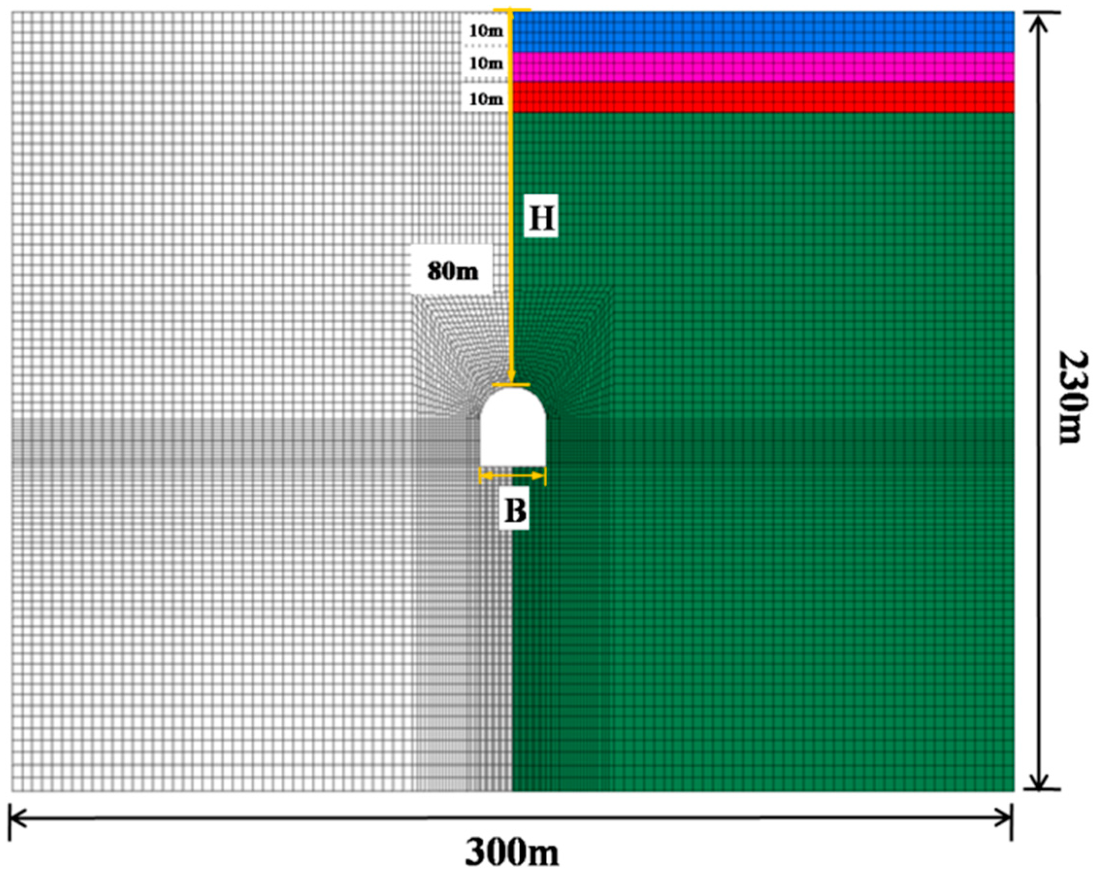
The numerical calculation model of the unit thickness was set as: height × width = 180 m × 300 m (210 m × 300 m, 240 m × 300 m, 270 m × 300 m). The element mesh and model dimension are shown in Figure 7.

H represents the vertical distance from the tunnel vault to the ground. The model’s boundary conditions were set so that the upper boundary was a free surface boundary, and both sides and the bottom edges were constrained by the method of normal displacement. The initial in situ stress was the self-weight stress of the rock mass.

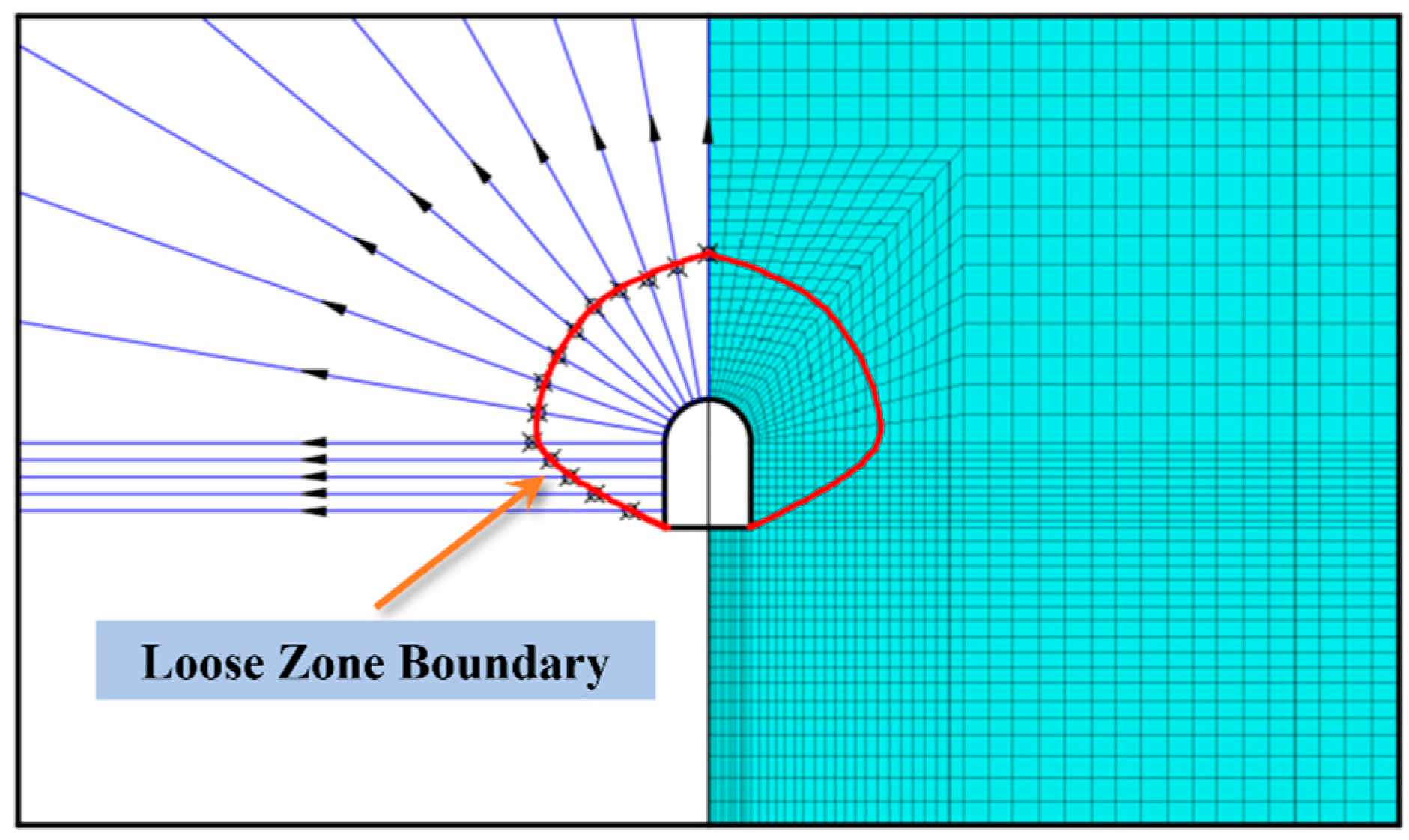
3.2.4. Method of Determining the Loose Zone in the Surrounding Rock Mass

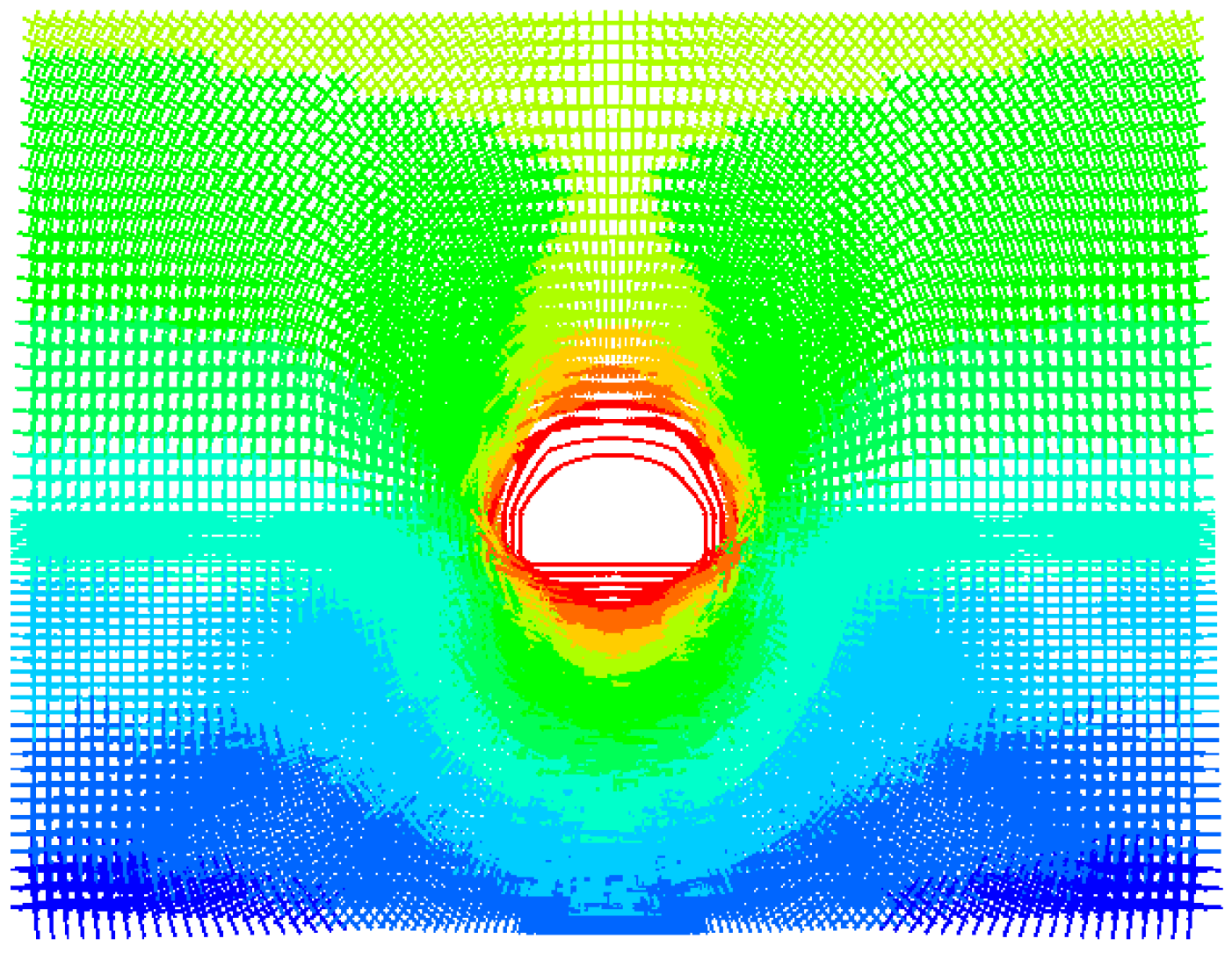
The pressure arch in the surrounding rock mass was characterized by an arch structure. The pressure arch body bears its own load and the load of the rock mass above the arch so that the surrounding rock maintains a certain degree of self-stability after excavation. However, the rock mass below the pressure arch has poor stability because it is close to the tunnel excavation outline, which leads to the stress exceeding the rock mass strength and causing damage. Therefore, the loose zone in the surrounding rock mass is defined as the rock mass from the inner boundary of the pressure arch to the tunnel contour. The principal stress vector diagram after the excavation of the No. 16 model is in Figure 8, showing the pressure arch shape and the ring-shaped distribution of the maximum principal stress.

Based on existing research results [34], this paper took the connection of the peak point of the surrounding rock’s tangential stress after the excavation of the tunnel as the judgment basis for the pressure arch inner boundary. The inner boundary criterion was embedded into FLAC3D with the Fish programming language to conduct numerical simulations. The correlation of the tangential stress can be calculated as follows:

$${\sigma }_{\theta }={\sigma }_x{\sin }^2\theta +{\sigma }_z{\cos }^2\theta -2{\tau }_{xz}\mathrm{s}\mathrm{i}\mathrm{n}\theta \mathrm{c}\mathrm{o}\mathrm{s}\theta$$

(5)

The simulation was processed as follows: ① The model was established according to the orthogonal test scheme and the initial stress field was calculated. ② The element stress component was extracted after the calculation was balanced and the tangential stress of each component was calculated using the correlation. ③ Values of the tangential stress of each element on the search path and were compared, and the element with the peak tangential stress point was marked. Owing to the model’s symmetry, half of the model was selected for the search. The specific shape of the loose zone was obtained by connecting the inner boundary position of the pressure arch on each search path. ④ The loose zone was smoothed by the least square method to obtain the final scope of the loose zone in the surrounding rock mass, as shown in Figure 9. It should be noted that the influence of floor heave was not considered in this study.

3.2.5. Analysis of the Factors Influencing the Loose Zone in the Surrounding Rock Mass

Three geometric quantities were selected as evaluation indexes reflecting the scope of the closed annular loose zone, namely $\mathit{L}$ (the span of the loose zone at the tunnel vault), ${\mathit{H}}_1$ (the height of the loose zone at the tunnel vault), and $\mathit{S}$ (the area of the loose zone). The geometric quantity diagram of the loose zone is shown in Figure 10. The data were processed for the 16 groups of working conditions, and the test number of the closed annular loose zone and the evaluation indexes of the loose zone scope were then summarized. The evaluation indexes of the loose area are shown in

Table 5. Summary of evaluation indexes of the loose area.

Model Number		1	2	3	4	5	6	7	8
Evaluation index	$L\left(\mathrm{m}\right)$	30.46	30.56	48.34	N/A	50.90	41.34	25.46	35.70
	$H_1\left(\mathrm{m}\right)$	17.25	9.77	11.19	N/A	7.04	11.30	3.11	12.67
	$S\left({\mathrm{m}}^2\right)$	239	207	336	N/A	470	203	104	228
Model Number		9	10	11	12	13	14	15	16
Evaluation index	$L\left(\mathrm{m}\right)$	41.02	50.50	N/A	61.58	45.30	58.50	39.78	65.46
	$H_1\left(\mathrm{m}\right)$	23.74	28.17	N/A	24.38	25.33	9.81	17.23	11.20
	$S\left({\mathrm{m}}^2\right)$	517	597	N/A	887	552	467	392	772

.

The CCR model quantitatively evaluates the factors influencing the loose zone in the surrounding rock mass using a fuzzy restriction on the weight [35]. This model can realize the evaluation and prediction of multi-index input and multi-index output problems with the help of the linear programming method. The model overcomes the shortcomings of the traditional CCR model, which discards influencing factors (the weight value is 0) when solving for optimal efficiency. The maximum fuzzy membership function constrains the upper and lower limits of the weight values to obtain the model’s optimal weight solution. The CCR model with a fuzzy restriction on the weight can be expressed as:

$$\left\{\begin{array}{l}\max \mu \\ \mathrm{s}.\mathrm{t}.{\displaystyle {\displaystyle \sum }_{r=1}^s}{u}_r{y}_{rj}-{\displaystyle {\displaystyle \sum }_{i=1}^m}{u}_r{x}_{ij}\le 0\left(j=\mathrm{1,2},\dots ,n\right)\\ \mu \cdot u_r^U\le u_r\le \left(1-\mu \right)\cdot u_r^U\left(r=\mathrm{1,2},\dots ,s\right)\\ \mu \cdot v_i^U\le v_i\le \left(1-\mu \right)\cdot v_i^U\left(i=\mathrm{1,2},\dots ,m\right)\end{array}\right.$$

(6)

where μ is the maximum fuzzy membership function; $y_{rj}$ is the output value of the r-th term; $x_{ij}$ is the input value of the i-th term; ${\mu }_r$ is the weight value of the r-th output; $v_i$ is the weight value of the i-th input; $u_r^U$ and $v_i^U$ are the upper limit values of the output weight and input weight, respectively.

When analyzing the factors influencing the loose pressure in the surrounding rock mass of a super-span tunnel, the input factors are H, B, λ, K, and GSI. The values of each impact factor are shown in Table 2. The output factors are L, $H_1$, and S, and their geometric statistics are shown in

Table 6. Weight value of influencing factors.

Influencing Factors	H	B	λ	K	GSI
Weight value	0.12	0.37	0.15	0.14	0.22

.

The weight values of the influencing factors are summarized in Table 1. It can be concluded that the order of the weight values of the influencing factors in the loose zone of a super-large section tunnel is $B>\mathrm{G}\mathrm{S}\mathrm{I}>K>\lambda >H$, which indicates that two factors (B for the tunnel span and GSI for surrounding rock quality) have a high degree of influence on the surrounding rock loose zone, while the other factors have less of an impact.

4. Boundary Function of the Surrounding Rock’s Loose Zone

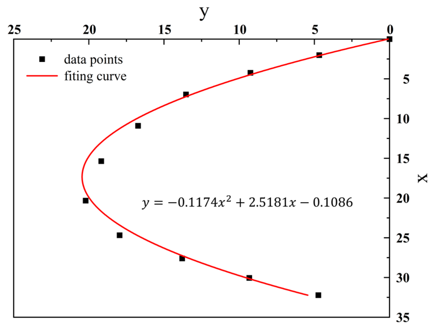
The boundary curve of the loose zone was fitted by a non-linear function based on the scope of the loose zone in the surrounding rock mass. Owing to the symmetry of the loose zone in the surrounding rock, half of the boundary curve was taken as the research object. The Cartesian rectangular coordinate system was adopted, taking the arch vertex of the loose zone as the coordinate origin. The positive direction on the X-axis was vertically downward, and the positive direction on the Y-axis was horizontal and to the left. Ten characteristic points were selected from the coordinate information on the boundary curve and were fitted by the built-in function in MATLAB according to the changing trend of data points to determine the boundary function of the loose zone. After data sorting and analysis, the quadratic function had the highest degree of fit for the dataset. Therefore, this paper took it as the boundary function with a, b, and c being undetermined coefficients. Taking Model 7 as an example, the fitting effect and relevant information are represented in Figure 11 and

Table 7. Results for the fitting curve.

Model Number	Formula	Undetermined Coefficient			Correlation Coefficient R2
		a	b	c
7	$y=a{x}^2+bx+c$.	−0.1174	2.5181	−0.1086	0.9988

.

The following can be concluded from the correlation between the evaluation indexes of the loose zone and the boundary function:

$$\left\{\begin{array}{l}x=0\Rightarrow y=0\\ x=-\frac{b}{2a}\Rightarrow y=\frac{1}{2}L\\ x=H_1+h\Rightarrow y=\frac{1}{2}B\end{array}\right.$$

(7)

Taking Correlation 5 into the boundary function $y=a{x}^2+bx+c$, the undetermined coefficients a, b, and c can be approximated:

$$\left\{\begin{array}{l}a=\frac{-L\times \left[1+{\left(1-\frac{B}{L}\right)}^{\frac{1}{2}}\right]}{{\left(H_1+h\right)}^2}\\ b=\frac{L\times \left[1+{\left(1-\frac{B}{L}\right)}^{\frac{1}{2}}\right]}{H_1+h}\\ c=0\end{array}\right.$$

(8)

Using the data in Table 3, Table 4 and Table 5, the multiple regression equations of $\mathit{L}$ and ${\mathit{H}}_1$ can be concluded via the process described below:

(1) Based on the principle of the least squares method, the univariate regression equation between the influencing factors of the loose zone with $\mathit{L}$ and ${\mathit{H}}_1$ are established, as shown in

Table 8. Unitary regression equation.

Factors	Formula	Correlation Coefficient R2
H	$L=78.28-67.87\times {0.9935}^H$	0.9986
	$H_1=19.15-65.12\times {0.9741}^H$	0.9433
B	$L=2.53+1.72B$	0.8477
	$H_1=7.98+1.01$B	0.8535
λ	$L=13.73+132.05\lambda -67.56{\lambda }^2$	0.9767
	$H_1=-23.74+71.88\lambda -35.18{\lambda }^2$	0.9978
K	$L=36.66-16.60\ln \left(K+0.2403\right)$	0.9991
	$H_1=17.89+4.49\ln \left(K-0.1532\right)$	0.8659
GSI	$L=41.63\times {\left(\mathrm{G}\mathrm{S}\mathrm{I}-24.45\right)}^{-0.05}$	0.8699
	$H_1=16.67\times {\left(\mathrm{G}\mathrm{S}\mathrm{I}-24.47\right)}^{-0.26}$	0.8904

. According to the manual, the correlation coefficient threshold value is 0.83. As illustrated in Table 8, the correlation coefficients of the five influencing factors all exceed 0.83, indicating that the univariate regression equations of $\mathit{L}$ and ${\mathit{H}}_1$ are correct.

(2) The prediction correlations for $\mathit{L}$ and ${\mathit{H}}_1$ can be deduced from the univariate regression equations as below:

$$\begin{array}{ll}& L=-46.63\times {0.9935}^H+1.16\times B+80.74\times \lambda -47.38\times {\lambda }^2+\\ & 6.76\times \mathrm{l}\mathrm{n}(K+0.2403)+1.99\times (\mathrm{GSI}-24.45{)}^{-0.05}+4.91\end{array}$$

(9)

$$\begin{array}{ll}& H_1=-37.56\times {0.9741}^H+1.10\times B+64.25\times \lambda -95.58\times {\lambda }^2+\\ & 7.44\times \mathrm{l}\mathrm{n}(K-0.1532)+23.73\times (\mathrm{GSI}-24.47{)}^{-0.26}-27.07\end{array}$$

(10)

The correctness of Correlation 7 and Correlation 8 are verified by the variance analysis, as shown in

Table 9. Variance analysis of multiple regression equation.

Variance Analysis of Correlation 7					Variance Analysis of Correlation 8
Source of Variance	Sum of Deviation Squares	Freedom	Mean Square	F	Source of Variance	Sum of Deviation Squares	Freedom	Mean Square	F
Regression	21391.7	6	1572.8	6.59	Regression	23964.4	6	1160.0	7.02
Error	3149.1	4	251.3	N/A	Error	3645.5	4	269.7	N/A
sum	24646.6	10	N/A	N/A	sum	29764.1	10	N/A	N/A

. The F distribution value is $\mathit{F}\left(\mathrm{6,4}\right)=6.59$ in Correlation 7 and $\mathit{F}\left(\mathrm{6,4}\right)=7.02$ in Correlation 8. Both are greater than ${\mathit{F}}_{0.05}\left(\mathrm{6,4}\right)=6.16$ at the 0.05 significance level, indicating that the accuracy of the regression equation meets the requirements.

It should be noted that the prediction correlations of $\mathit{L}$ and ${\mathit{H}}_1$ were established with $80 \mathrm{m}\le H\le 110 \mathrm{m}$, $20 \mathrm{m}\le B\le 35 \mathrm{m}$, $0.6\le \lambda \le 1.2$, $0.5\le K\le 2.0$, $\mathrm{a}\mathrm{n}\mathrm{d}25\le \mathrm{G}\mathrm{S}\mathrm{I}\le 40$. The parameter values must be defined within the domain.

5. Upper Bound Solution for Loose Pressure in the Surrounding Rock Mass

5.1. Upper Boundary Solution for Loose Pressure for Extra-Large Section Tunnels

5.1.1. Basic Assumptions

Four basic assumptions must be made when the upper bound theory is applied to analyze and calculate the loose pressure of surrounding rock:

① The rock–soil mass is regarded as a perfectly elastic–plastic material that obeys the H-B yield criteria.

② The tunnel arch is under a vertical even load q, and the side walls are under a horizontal even load e. Assuming that q is proportional to e, the proportional coefficient is the side pressure coefficient K, that is, $e=Kq$

③ The influences of the construction process and floor heave are not considered.

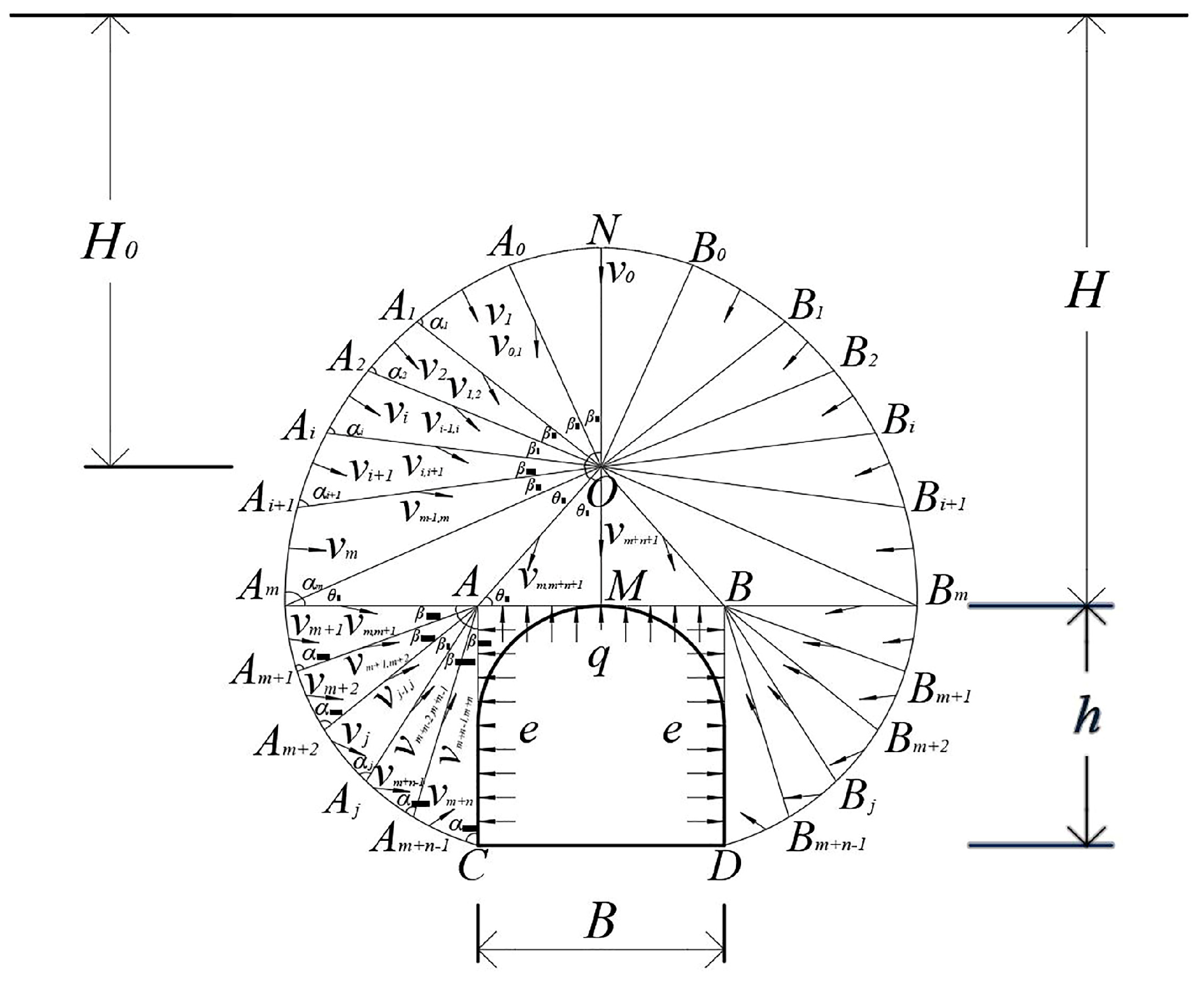
5.1.2. Description of Failure Mechanism

The basic shape of the loose zone obtained from the orthogonal test shows that the failure forms of the deeply buried tunnel include the tunnel vault subsidence and side wall shrinkage. Based on the determination of the failure zone, the mass of rock and soil in the failure mechanism is divided into rigid blocks that meet the conditions. The velocity and direction of each rigid block are obtained according to the geometric relationship and the sine theorem corresponding to the failure mechanism.

In summary, the failure mechanism of a deeply buried tunnel is represented in Figure 12. The tunnel section is approximately rectangular, ABCD, with height h and span B. M and N are located at the midpoint of the tunnel vault and the midpoint of the loose zone boundary curve, respectively. O is located on the straight line MN and is the auxiliary point. H represents the burial depth of the cavity $H_1$ represents the distance from O to the ground plane, and the support reaction forces of the tunnel arch and the side walls are the uniform loads q and e, respectively.

Owing to the symmetry of the failure mechanism, this study takes the left half of the failure mechanism for the corresponding description. $AB$ is extended to intersect the boundary curve at point $A_m$. $\angle A_{m}ON$ is divided into $m+1$ parts with angles for ${\beta }_0,{\beta }_1,\dots ,{\beta }_m$. $\angle {AA}_{m}C$ is divided into n parts with angles ${\beta }_{m+1},{\beta }_{m+2},\dots ,{\beta }_{m+n}$. The intersections of each angle and the boundary of the loose zone are recorded as $A_0,A_1,\dots ,A_m,\dots ,A_{m+n+1}$. Connecting $N{A}_0,A_0{A}_1,A_1{A}_2,\dots ,A_m{A}_{m+1},\dots ,A_{m+n-1}C$, when m and n are large enough, the error between each connecting line and the boundary curve is therefore small enough.

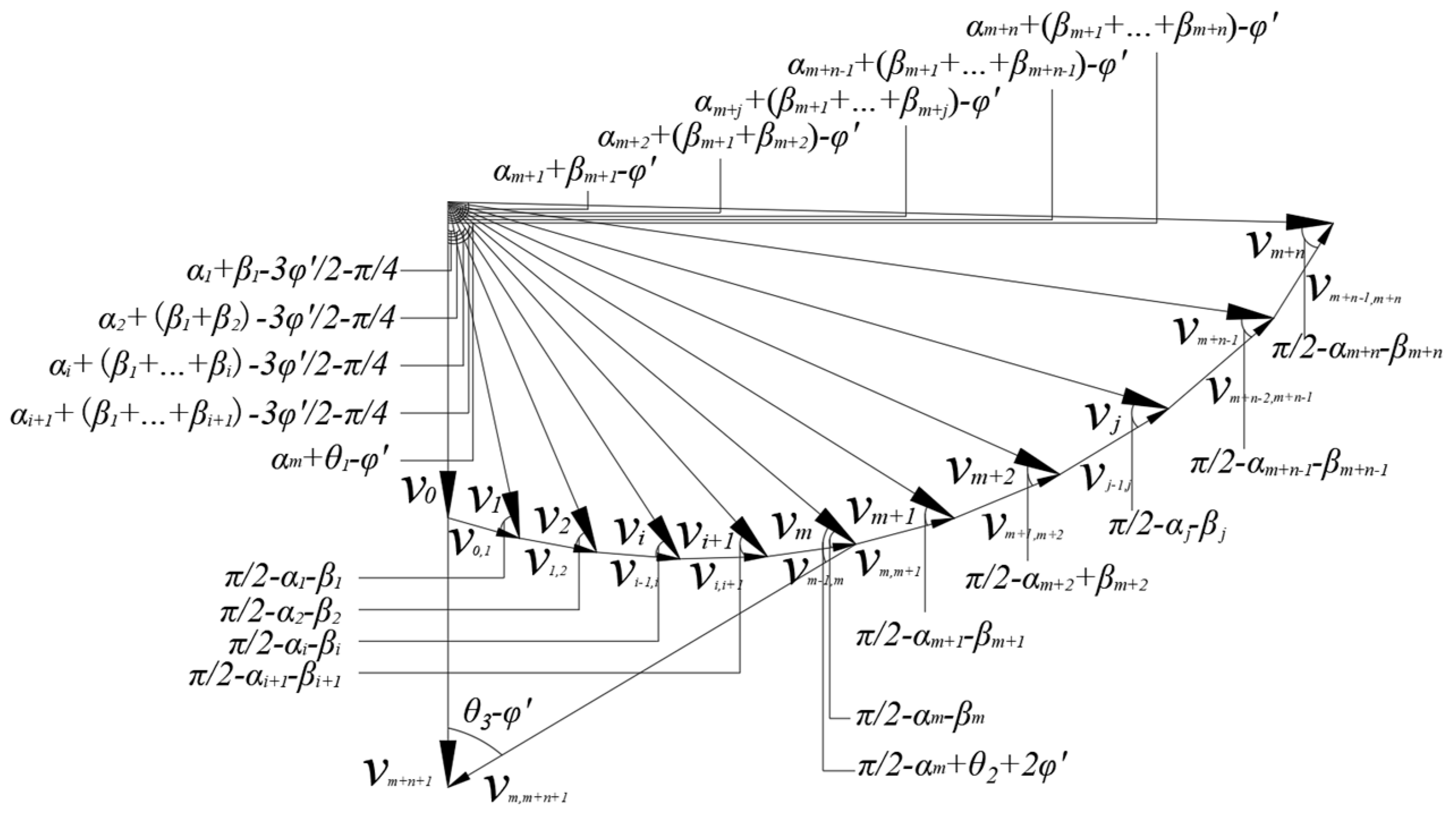
According to the associated flow rule, the velocity vector sum of the rigid slider is zero, and the angle between the relative velocity vector and the discontinuity line should be $\phi \prime$. Figure 13 shows the kinematically admissible velocity field corresponding to the failure mechanism. The velocity of block $∆A_{0}ON$ is $V_0$ in the vertically downward direction. The velocity of block $∆AOM$ is $V_{m+n+1}$ in the vertically downward direction. The velocities of the other blocks, from top to bottom, are $V_1,\dots V_{m+n},$ and the relative velocities of each rigid slider on the discontinuity line are $V_{\mathrm{0,1}},\dots ,V_{m+n-1,m+n},V_{m+n,m+n+1}$. The shape of the blocks is determined by ${\alpha }_1,\dots ,{\alpha }_m$ and ${\beta }_1,\dots ,{\beta }_m$. With reference to Protodyakonov’s theory and the Terzaghi theory, the shapes can be assumed to be ${\beta }_0=\pi /4-\phi \mathrm{\prime }/4$.

5.1.3. Derivation of the Upper Bound Solution for the Loose Pressure

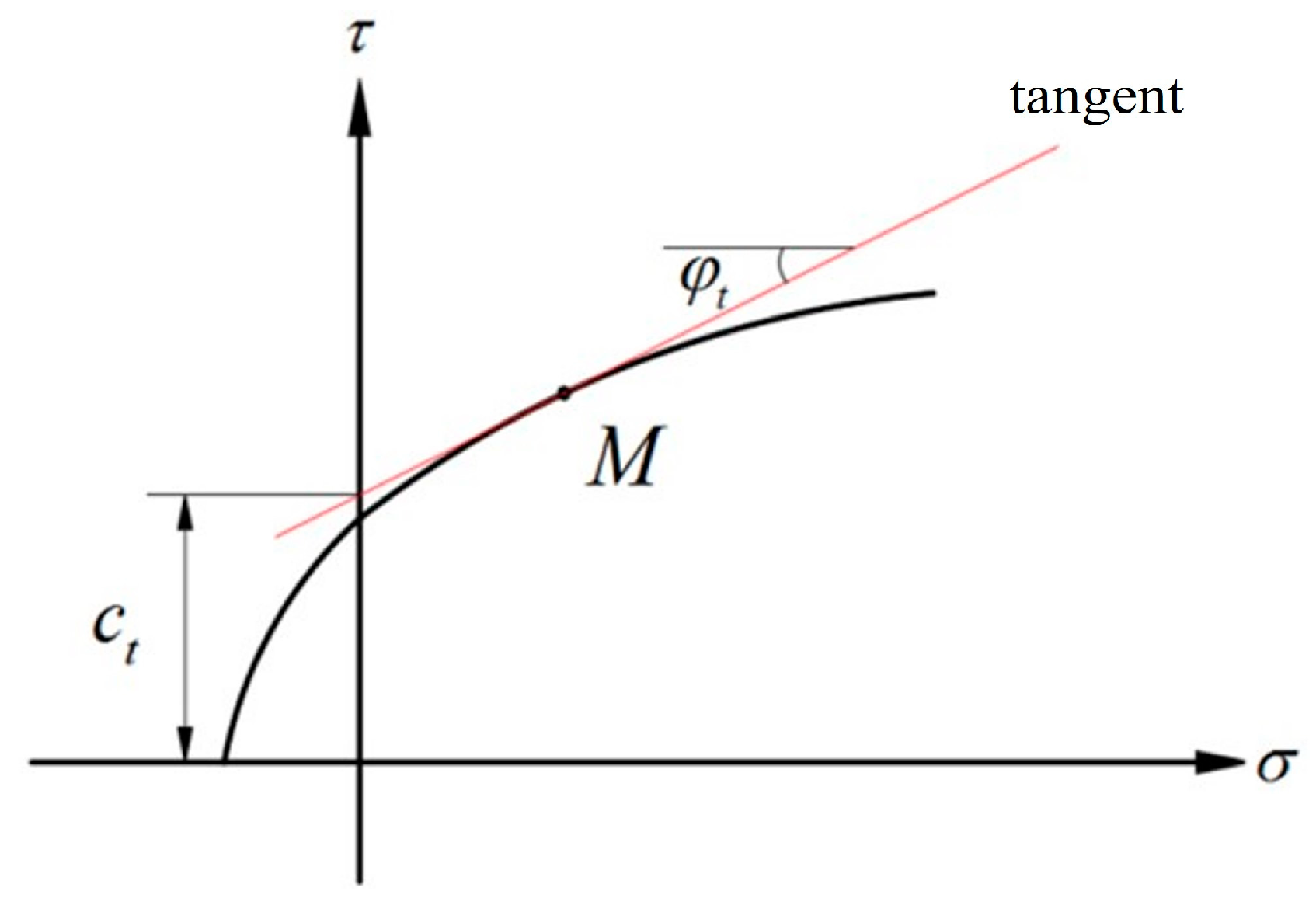
(1) Limit Analysis Based on H-B Strength Criterion

Based on the assumptions mentioned above, the loose zone is regarded as an ideal elastic–plastic body which obeys the H-B criterion. The relation between $c_t$ and ${\phi }_t$ can be obtained as below using the tangent method (Figure 14) [36]:

$$\frac{c_t}{{\phi }_t}=\frac{\cos {\phi }_t}{2}{\left[\frac{m_b\left(1-\sin {\phi }_t\right)}{2\sin {\phi }_t}\right]}^{\frac{a}{1-a}}-\frac{\tan {\phi }_t}{m_b}\left(1+\frac{\sin {\phi }_t}{a}\right){\left[\frac{m_b\left(1-\sin {\phi }_t\right)}{2\sin {\phi }_t}\right]}^{\frac{a}{1-a}}+\frac{s}{m_b}$$

(11)

The non-linear shear strength index ${\phi }_t$ in the above correlations serves as an unknown parameter in the upper-bound limit analysis, reflecting the instantaneous variability of the tangent, which is obtained by the optimization algorithm. $c_t$ is obtained by Correlation 10 after ${\phi }_t$ is determined.

(2) Calculation of geometric quantities

Owing to the symmetry of the failure mechanism, this paper takes the left part of MN as an example for geometric quantity calculation. The point N is taken as the coordinate origin and a rectangular coordinate system is established. The vertical is the X-axis, where the down is positive, and the horizontal direction is the Y-axis, where the left is positive. According to the loose zone boundary equation, the expression of the curve NC is $y=a{x}^2+bx+c$.

According to the relevant description of failure mechanism and the research results of the loose zone in the surrounding rock mass, it can be known that $\left|AM\right|=B/2$, $\left|AC\right|=h$, $\left|A_{m}M\right|=L/2$, $\left|MN\right|=H$, $\left|OM\right|=H-H_0$, $\left|ON\right|=H_1-H+H_0$.

It can be concluded from the trigonometric function:

$$\left\{\begin{array}{c}{\theta }_1=\mathrm{a}\mathrm{r}\mathrm{c}\mathrm{t}\mathrm{a}\mathrm{n}\left[2\left(H-H_0\right)/L\right]\\ {\theta }_4=\mathrm{a}\mathrm{r}\mathrm{c}\mathrm{t}\mathrm{a}\mathrm{n}\left[2\left(H-H_0\right)/B\right]\end{array}\right.$$

(12)

The linear equations of $O{A}_0,O{A}_1,\dots ,O{A}_m$ can be obtained from the coordinate $\left(H_1-H+H_0,O\right)$ of point $O$ and the division of $\angle A_{m}ON$ as follows:

$$\left\{\begin{array}{l}y=\tan \left[\pi -\left(\frac{\pi }{4}-\frac{\phi }{2}\right)\right]\cdot \left[x-\left(H_1-H+H_0\right)\right]\\ y=\tan \left[\pi -\left(\frac{\pi }{4}-\frac{\phi }{2}\right)-{\beta }_1\right]\cdot \left[x-\left(H_1-H+H_0\right)\right]\\ \cdots \\ y=\tan \left[\pi -\left(\frac{\pi }{4}-\frac{\phi }{2}\right)-{\displaystyle {\displaystyle \sum }_{\mathrm{i}=1}^{\mathrm{m}}}{\beta }_i\right]\cdot \left[x-\left(H_1-H+H_0\right)\right]\end{array}\right.$$

(13)

The linear equations of $A{A}_{m+1},A{A}_{m+2},\dots ,A{A}_{m+n-1}$ can be obtained from the coordinate $\left(H,B/2\right)$ of point $A$ and the division of $\angle A{A}_{m}C$ as follows:

$$\left\{\begin{array}{l}y=\tan \left(\frac{\pi }{2}-{\beta }_{m+1}\right)\cdot \left(x-H\right)+\frac{B}{2}\\ y=\tan \left(\frac{\pi }{2}-{\beta }_{m+1}-{\beta }_{m+2}\right)\cdot \left(x-H\right)+\frac{B}{2}\\ \cdots \\ y=\tan \left(\frac{\pi }{2}-{\displaystyle {\displaystyle \sum }_{i=m+1}^{m+n-1}}{\beta }_i\right)\cdot \left(x-H\right)+\frac{B}{2}\end{array}\right.$$

(14)

The coordinates $\left(x_0,y_0\right),\left(x_1,y_1\right),...,\left(x_{m+n-2},y_{m+n-2}\right),\left(x_{m+n-1},y_{m+n-1}\right)$ of $A_0,A_1,\dots ,A_m,\dots ,A_{m+n-1}$ can be obtained by combining the loose zone boundary equation with the linear equations, and the following correlations calculate the distance of each line segment:

$$\left\{\begin{array}{l}\left|N{A}_0\right|=\sqrt{x_0^2+y_0^2}\\ \left|A_i{A}_{i+1}\right|=\sqrt{{\left(x_{i+1}-x_i\right)}^2+{\left(y_{i+1}-y_i\right)}^2},(i=\mathrm{0,1},\dots ,m+n-2)\\ \left|A_{m+n-1}C\right|=\sqrt{{\left[x_{m+n-1}-\left(H_1+h\right)\right]}^2+{\left(y_{m+n-1}-B/2\right)}^2}\\ \left|O{A}_1\right|=\sqrt{{\left[x_i-\left(H_1-H+H_0\right)\right]}^2+y_j^2},(i=\mathrm{0,1},\dots ,m)\\ \left|A{A}_j\right|=\sqrt{{\left(x_j-H_1\right)}^2+{\left(y_j-B/2\right)}^2},(i=m+1,m+2,\dots ,m+n-1)\\ \left|OA\right|=\sqrt{{\left(H-H_1\right)}^2+B^2/4}\end{array}\right.$$

(15)

${\alpha }_1,\dots ,{\alpha }_{m+n}$ can be calculated by the sine theorem:

$$\left\{\begin{array}{l}{\alpha }_1=\arcsin \left(\left|\frac{O{A}_0}{A_0{A}_1}\right|\sin {\beta }_1\right)\\ {\alpha }_i=\arcsin \left(\left|\frac{A{A}_{i-1}}{A_{i-1}{A}_i}\right|\sin {\beta }_i\right),\left(i=2,\dots ,m\right)\\ {\alpha }_j=\arcsin \left(\left|\frac{A{A}_{j-1}}{A_{j-1}{A}_j}\right|\sin {\beta }_j\right),\left(j=m+1,\dots ,m+n-1\right)\\ {\alpha }_{m+n}=\arcsin \left(\left|\frac{CA}{A_{m+n-1}C}\right|\sin {\beta }_{m+n}\right)\end{array}\right.$$

(16)

(3) Calculation of the velocity field

As seen in Figure 13, the velocity vector relationship of each slider meets the following recurrence correlations:

$$V_1=\frac{\mathrm{s}\mathrm{i}\mathrm{n}\left(3\pi /4+3{\phi }_t/2\right)}{\mathrm{s}\mathrm{i}\mathrm{n}\left(\pi /2-{\alpha }_1-{\beta }_1\right)}{V}_0$$

(17)

$$V_{\mathrm{0,1}}=\frac{\mathrm{s}\mathrm{i}\mathrm{n}\left({\alpha }_1+{\beta }_1-3{\phi }_t/2-\pi /4\right)}{\mathrm{s}\mathrm{i}\mathrm{n}\left(\pi /2-{\alpha }_1-{\beta }_1\right)}{V}_0$$

(18)

$$V_{i+1}=\frac{\mathrm{s}\mathrm{i}\mathrm{n}\left(\pi /2-{\alpha }_{i+1}\right)}{\mathrm{s}\mathrm{i}\mathrm{n}\left(\pi /2-{\alpha }_{i+1}-{\beta }_{i+1}\right)}{V}_i(i=1,\dots ,m-1)$$

(19)

$$V_{i,i+1}=\frac{\sin \left({\alpha }_{i+1}-{\alpha }_i+{\beta }_{i+1}\right)}{\sin \left(\pi /2-{\alpha }_{i+1}-{\beta }_{i+1}\right)}{V}_i(i=1,\dots ,m-1)$$

(20)

$$V_{m+1}=\frac{\mathrm{s}\mathrm{i}\mathrm{n}\left(\pi /2+{\alpha }_{m+1}+{\theta }_1\right)}{\mathrm{s}\mathrm{i}\mathrm{n}\left(\pi /2-{\alpha }_{m+1}-{\beta }_{m+1}\right)}{V}_m$$

(21)

$$V_{m,m+1}=\frac{\mathrm{s}\mathrm{i}\mathrm{n}\left({\alpha }_{m+1}-{\alpha }_m+{\beta }_{m+1}-{\theta }_1\right)}{\mathrm{s}\mathrm{i}\mathrm{n}\left(\pi /2-{\alpha }_{m+1}-{\beta }_{m+1}\right)}{V}_m$$

(22)

$$V_{j+1}=\frac{\mathrm{s}\mathrm{i}\mathrm{n}\left(\pi /2-{\alpha }_{j+1}\right)}{\mathrm{s}\mathrm{i}\mathrm{n}\left(\pi /2-{\alpha }_{j+1}-{\beta }_{j+1}\right)}{V}_j(j=m+1,\dots ,m+n-1)$$

(23)

$$V_{j,j+1}=\frac{\mathrm{s}\mathrm{i}\mathrm{n}\left({\alpha }_{j+1}-{\alpha }_j+{\beta }_{j+1}\right)}{\mathrm{s}\mathrm{i}\mathrm{n}\left(\pi /2-{\alpha }_j-{\beta }_j\right)}{V}_j(j=m+1,\dots ,m+n-1)$$

(24)

$$V_{m+n+1}=\frac{\mathrm{s}\mathrm{i}\mathrm{n}\left(\pi /2-{\alpha }_m+{\theta }_4-{\theta }_1+2{\phi }_t\right)}{\mathrm{s}\mathrm{i}\mathrm{n}\left(\pi /2-{\theta }_4-{\phi }_t\right)}{V}_m$$

(25)

$$V_{m,m+n+1}=\frac{\mathrm{s}\mathrm{i}\mathrm{n}\left({\alpha }_m+{\beta }_{m+1}-{\phi }_t\right)}{\mathrm{s}\mathrm{i}\mathrm{n}\left(\pi /2-{\theta }_4-{\phi }_t\right)}{V}_m$$

(26)

(4) Calculation of external powers

① Power of gravitational force

$$S_{△NO{A}_0}=1/2\left|NO\right|\cdot \left|A_{0}O\right|\mathrm{s}\mathrm{i}\mathrm{n}{\beta }_0$$

(27)

$$S_{△A_{i}O{A}_{i+1}}=1/2\left|A_{i}O\right|\cdot \left|A_{i+1}O\right|\mathrm{s}\mathrm{i}\mathrm{n}{\beta }_{i+1}(i=0,\dots ,m-1)$$

(28)

$$S_{△A_{m}OA}=1/2\left|A_{m}A\right|\cdot \left|OM\right|=1/4(L-B)\cdot \left(H-H_0\right)$$

(29)

$$S_{△AOM}=1/2\left|AM\right|\cdot \left|OM\right|=1/4D\cdot \left(H-H_0\right)$$

(30)

$$S_{△A_{j}A{A}_{j+1}}=1/2\left|A_{j}A\right|\cdot \left|A_{j+1}A\right|\mathrm{s}\mathrm{i}\mathrm{n}{\beta }_{j+1}(j=m,\dots ,m+n-2)$$

(31)

$$S_{\mathsf{\Delta }{A}_{m+n-1}AC}=1/2\left|A_{m+n+1}A\right|\cdot \left|AC\right|\mathrm{s}\mathrm{i}\mathrm{n}{\beta }_m=h/2\cdot \left|A_{m+n+1}A\right|\cdot \mathrm{s}\mathrm{i}\mathrm{n}{\beta }_m$$

(32)

Gravitational power generated by each rigid slider:

$$W_0=S_{△NO{A}_0}\cdot \gamma \cdot V_0$$

(33)

$$W_i=S_{△A_{i}O{A}_{i-1}}\cdot \gamma \cdot V_i\cdot \mathrm{c}\mathrm{o}\mathrm{s}({\alpha }_i+{\sum }_{k=1}^i{\beta }_k-3{\phi }_t/2-\pi /4)(i=1,\dots ,m-1)$$

(34)

$$W_m=\left(S_{△A_{m-1}O{A}_m}+S_{△A_{m}OA}\right)\cdot \gamma \cdot V_m\cdot \cos \left({\alpha }_m+{\theta }_1-{\phi }_t\right)$$

(35)

$$W_i=S_{\mathsf{\Delta }{A}_{j}A{A}_{j-1}}\cdot \gamma \cdot V_j\cdot \cos ({\alpha }_j+{\sum }_{k=m+1}^j{\beta }_k-{\phi }_t)(j=m+1,\dots ,m+n)$$

(36)

$$W_{m+n+1}=S_{△AOM}\cdot \gamma \cdot V_{m+n+1}$$

(37)

② Power of Support Reaction

$$W_T=-q\cdot B/2\cdot V_0-K\cdot q\cdot h\cdot \sin \left({\alpha }_{m+n}-{\phi }_t\right)\cdot V_{m+n+1}$$

(38)

(5) Power of Internal Energy Dissipation

$$P_1=c_t\cdot \cos {\phi }_t\cdot \left|A_{0}N\right|\cdot V_0$$

(39)

$$P_2=c_t\cdot \cos {\phi }_t\cdot {\displaystyle {\displaystyle \sum }_{i=1}^{m-1}}\left(\left|A_{i-1}{A}_i\right|\cdot V_i+\left|A_{i-1}O\right|\cdot V_{i-1,i}\right)$$

(40)

$$P_3=c_t\cdot \cos {\phi }_t\cdot \left(\left|A_0{A}_{m-1}\right|\cdot V_m+\left|A_{m-1}O\right|\cdot V_{m-1,m}\right)$$

(41)

$$P_4=c_t\cdot \cos {\phi }_t\cdot {\displaystyle {\displaystyle \sum }_{j=m+1}^{m+n-1}}\left(\left|A_{j-1}{A}_j\right|\cdot V_j+\left|A_{j-1}O\right|\cdot V_{j-1,j}\right)$$

(42)

$$P_5=c_t\cdot \cos {\phi }_t\cdot \left(\left|A_{m+n-1}C\right|\cdot V_{m+n}+\left|A_{m+n-1}A\right|\cdot V_{m+n-1,m+n}\right)$$

(43)

$$P_6=c_t\cdot \cos {\phi }_t\cdot \left|OA\right|\cdot V_{m,m+n+1}$$

(44)

Power of Total Internal Energy Dissipation:

$$D_{\mathrm{int}}=P_1+P_2+P_3+P_4+P_5+P_6$$

(45)

(6) Calculation of support reaction

Based on the virtual work principle, the power produced by the external force is equal to the power dissipated by the internal energy.

$${\displaystyle {\displaystyle \sum }_{i=0}^{m+n+1}}{W}_i+W_T=D_{\mathrm{int}}$$

(46)

The correlation of the loose pressure in the surrounding rock mass is:

$$q=\frac{{\sum }_{i=0}^{m+n+1}{W}_i-\left(P_1+P_2+P_3+P_4+P_5+P_6\right)}{q\cdot B/2\cdot V_0+K\cdot q\cdot h\cdot \sin \left({\alpha }_{m+n}-{\phi }_t\right)\cdot V_{m+n+1}}$$

(47)

To ensure the velocity vector closure, each angle in the failure mechanism must meet the following constraints [37]:

$$\left\{\begin{array}{l}{\alpha }_1+{\beta }_1-\frac{3{\phi }_t}{2}-\frac{\pi }{4}>0\\ {\alpha }_{i+1i}+{\beta }_{i+1}>\alpha \left(i=1,\dots ,m-1\right)\\ {\alpha }_{j+1j}+{\beta }_{j+1}>\alpha \left(j=m+1,\dots ,m+n-1\right)\\ \frac{\pi }{2}-{\alpha }_k>{\beta }_k\left(k=1,\dots ,m+n\right)\\ {\alpha }_m+{\theta }_1>{\phi }_t\\ \frac{\pi }{2}+{\alpha }_m+{\theta }_1>0\\ {\alpha }_{m+1}+{\beta }_{m+1}-{\alpha }_m>{\theta }_1\\ \frac{\pi }{2}-{\theta }_4-{\phi }_t>0\\ \frac{\pi }{2}-{\alpha }_m+{\theta }_4-{\theta }_1+2{\phi }_t>0\\ {\alpha }_{m+1}-{\phi }_t+{\beta }_{m+1}>0\\ {\displaystyle {\displaystyle \sum }_{p=1}^m}{\beta }_p-\frac{{\phi }_t}{2}-{\theta }_1=\frac{\pi }{4}\end{array}\right.$$

(48)

With the commands of the MATLAB optimization toolbox utilized and the constraints met, a certain number of the loose pressure values in the surrounding rock mass are obtained in which the maximum value is the upper bound solution for the loose pressure in the surrounding rock mass.

The horizontal support reaction can be calculated as:

$$e=K\cdot q$$

(49)

5.2. Upper Boundary Solution for Loose Pressure for Extra-Large Section Tunnels

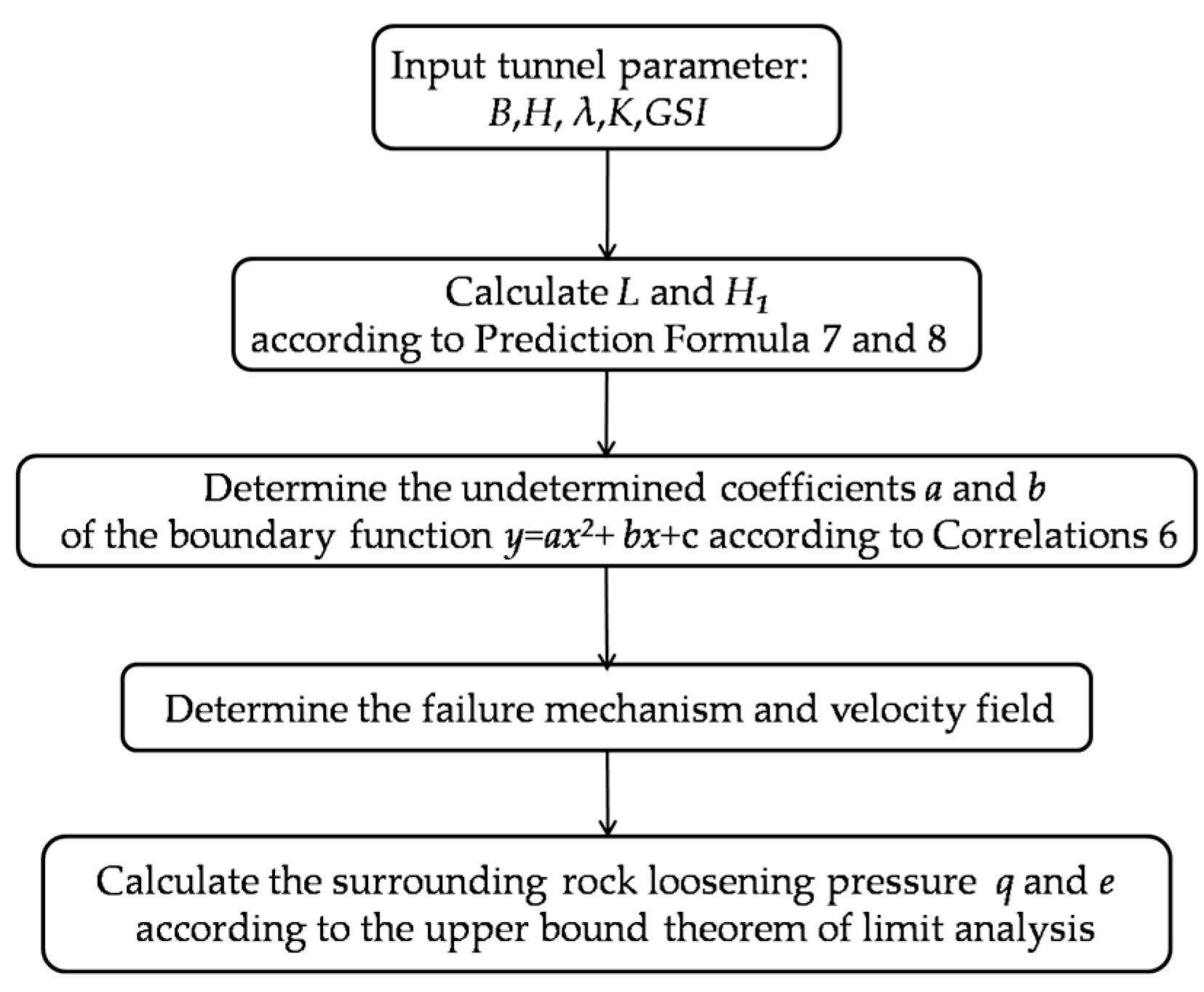
Based on the above research results, the process of calculating the loose pressure for a super-span tunnel is represented in Figure 15. The loose pressure of the large-span section (the maximum Section, Gradient Section 1, and Gradient Section 2) was calculated according to the calculation process outlined above, with the geological conditions of the tunnel taken into consideration. The calculation parameters and the calculation results are represented in

Table 10. Calculation parameters.

Section Size	GSI	H (m)	B (m)	λ	K
Maximum section	40	104	30.01	0.61	0.50
Gradient Section 1	40	90	27.16	0.65	0.50
Gradient Section 2	28	82	23.62	0.70	0.50

and

Table 11. Loose pressure in the surrounding rock mass based on the upper bound analysis.

Section Size	Evaluation Index		Boundary Function	Surrounding Rock Loose Pressure
	L/m	H1/m		Vault Vertical Pressure (kPa)	Haunch Horizontal Pressure (kPa)
Maximum Section	40.54	9.8	$y=-0.060x^2+2.202x$	269.44	134.72
Gradient Section 1	36.72	9.2	$y=-0.058x^2+2.061x$	243.36	121.68
Gradient Section 2	41.26	12.6	$y=-0.074x^2+2.472x$	307.11	153.56

, respectively.

5.3. Comparison between the Correlation Results and In Situ Measured Values

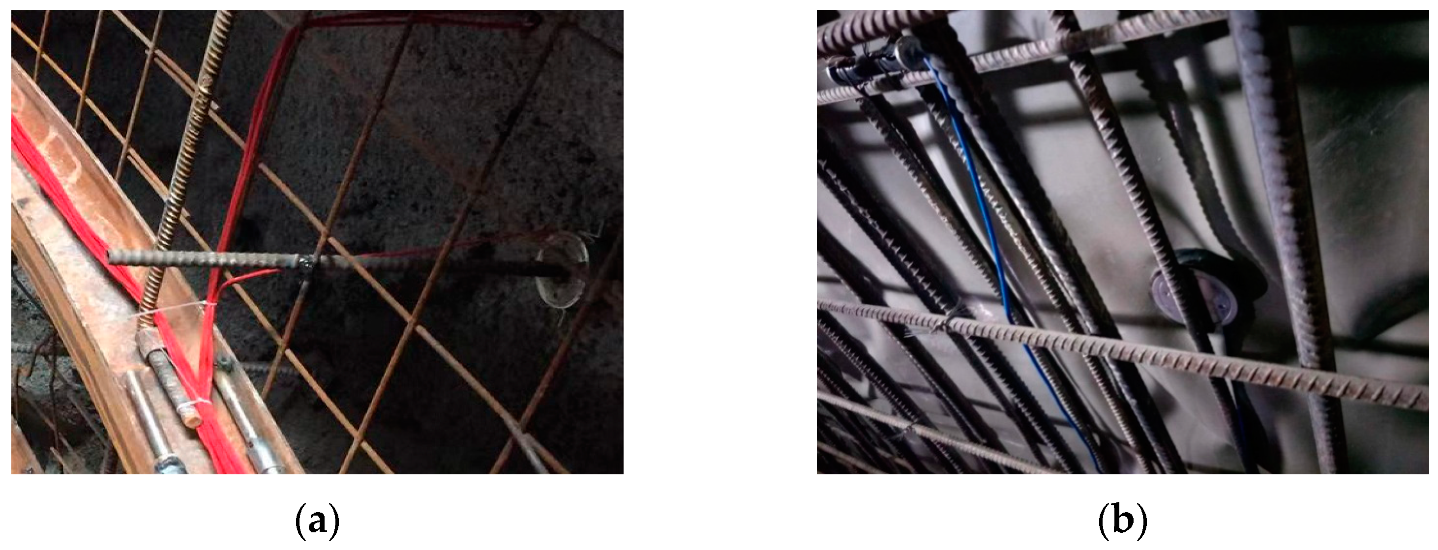
Several difficulties and risks existed in the construction of the super-large section. In order to ensure the construction quality and grasp the distribution pattern of the surrounding rock pressure, our research group conducted a half-year on-site monitoring of the large-span section from April 2018 to October 2018. The monitoring items included the displacement of the deep surrounding rock, the contact pressure between the surrounding rock and the structure’s steel, and the stress of steel arch. The Maximum Section, the Gradient Section 1 and the Gradient Section 2 were selected as surrounding rock pressure monitoring sections. The site photos of the earth pressure cell are represented in Figure 16.

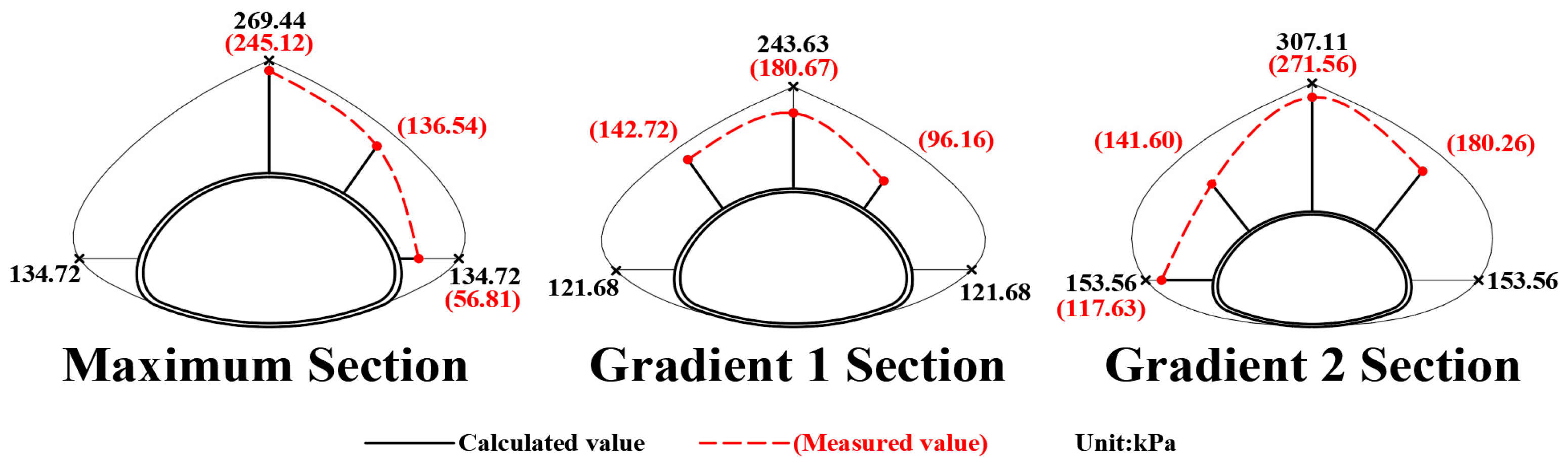
The stable values of the loose pressure of each monitoring section’s surrounding rock were collected to determine the circumferential distribution. They were then compared with the value calculated for the loose pressure in the surrounding rock mass based on the upper bound limit analysis method, as shown in Figure 17. The figure shows that the distribution law of the surrounding rock’s calculated loose pressure is consistent with the measured results except for the right side of the maximum section. The main reason for monitoring data distortion at the right side of the maximum section was the failure to install pressure sensors in a timely manner after excavation. As the surrounding rock pressure is monitored after the completion of the supporting structure, the monitoring results are the variation relative to the initial stress, and the monitoring values are usually less than the theoretical calculation values. As illustrated in Figure 17, the calculated results have a good envelope effect on the measured data, which proves the correctness and practicability of the calculation method.

6. Conclusions

(1) With the combination of a numerical analysis and an orthogonal test, the factors affecting the loose zone range of the surrounding rock were studied. According to CCR model with fuzzy restrictions on the weight in statistics, the order of factors influencing the weight value from large to small is $B>\mathrm{G}\mathrm{S}\mathrm{I}>K>\lambda >H$.

(2) The loose boundary zone expression of a deeply buried tunnel was determined to be $y=a{x}^2+bx+c$, and a calculation method for the undetermined coefficients of the boundary expression was proposed. The correlations of typical geometric quantities $\mathit{L}$ and ${\mathit{H}}_1$, representing the loose zone range, were established based on the unitary regression equations between the factors affecting the loose zone and typical geometric quantities.

(3) Based on the boundary function of the loose zone and the upper bound limit analysis method, a limit analysis model of the loose pressure in the surrounding rock mass under a non-linear failure criterion was established via the tangent method and virtual power principle, and the correlations of the loose pressure were deduced. The calculated values of the loose pressure were consistent with the pressure-monitoring results in the different sections of the large-span section, verifying the correctness of the proposed calculation method. The research results can provide new ideas for the selection of a supporting structure for similar super-section tunnel projects.

7. Discussion

(1) The orthogonal test designed in this paper considers several influence factors, and the value range is small (e.g., H is only 80~110 m.). In follow-up research, parameters such as the structural plane of the rock mass will be included in the influencing factors to improve the applicability of the calculation method.

(2) To simplify the analysis process, heterogeneities within the stratum were not considered in the study.

(3) The failure mechanism proposed in this paper did not consider the situation of floor heave, which must be improved in future research.

References

- Gu, Z.Q.; Peng, S.Z.; Li, Z.K. Underground Cavern Engineering; Tsinghua University Press: Beijing, China, 1994; pp. 50–53. [Google Scholar]
- Bierbaumer, A. Diedimensionerung des Tunnelmauerwerks; Engelmann: Leipzig, Germany, 1913. [Google Scholar]
- Terzaghi, K. Theoretical Soil Mechanics; John Wiley and Sons, Inc.: Hoboken, NJ, USA, 1943. [Google Scholar]
- Xie, J. Earth Pressure on Shallow Burial Tunnel. China Civil Eng. J. 1964, 6, 58–70. [Google Scholar]
- TB10003; Code for Design of Railway Tunnels. China Railway Publishing House: Beijing, China, 2005.
- JTG D70-2010; Code for Design of Road Tunnels. People’s Communications Publishing House: Beijing, China, 2004.
- SL279; Code for Design of Hydraulic Tunnels. China Water & Power Press: Beijing, China, 2002.
- Chongqing Civil Engineering Institute. Underground Construction in Rock; China Architecture & Building Press: Beijing, China, 1982. [Google Scholar]
- Barton, N.; Lien, R.; Lunde, J. Engineering classification of rock masses for the design of tunnel support. Rock Mech. 1974, 6, 183–236. [Google Scholar] [CrossRef]
- Bhasin, R.; Grimstad, E. The Use of Stress-Strengh Relationship in the Assessment of Tunnel Stability. Proc. Recent Adv. Tunn. Technol. 1996, 11, 93–98. [Google Scholar]
- Unal, E. Development of Design Guidelines and Roof-Control Standards for Coal-Mine Roofs; Pennsylvania State University: State College, PA, USA, 1983. [Google Scholar]
- Goel, R.K.; Jethwa, J.L. Prediction of Support Pressure using RMR Classification. In Proceedings of the Indian Geotechnical Conference, Surat, India, 20–22 December 1991. [Google Scholar]
- Atkinson, J.H.; Potts, D.M. Stability of a shallow circular tunnel in cohesion-less soil. Geotechnique 1977, 27, 203–215. [Google Scholar] [CrossRef]
- Davis, E.H.; Gunn, M.J.; Mair, R.J.; Seneviratine, H.N. The stability of shallow tunnels and underground openings in cohesive material. Geotechnique 1980, 30, 397–416. [Google Scholar] [CrossRef]
- Mollon, G.; Dias, D.; Soubra, A.H. Face stability analysis of circular tunnels driven by a pressurized shield. J. Geotech. Geoenvironmental Eng. 2010, 136, 215–229. [Google Scholar] [CrossRef]
- Mollon, G.; Dias, D.; Soubra, A.H. Rotational failure mechanisms for the face stability analysis of tunnels driven by a pressurized shield. Int. J. Numer. Anal. Methods Geomech. 2011, 35, 1363–1388. [Google Scholar] [CrossRef]
- Huang, F.; Yang, X.L. Upper bound limit analysis of collapse shape for circular tunnel subjected to pore pressure based on the Hoek–Brown failure criterion. Tunn. Undergr. Space Technol. Inc. Trenchless Technol. Res. 2011, 26, 614–618. [Google Scholar] [CrossRef]
- Lei, M.; Peng, L.; Shi, C. Calculation of the surrounding rock pressure on a shallow buried tunnel using linear and nonlinear failure criteria. Autom. Constr. 2014, 37, 191–195. [Google Scholar] [CrossRef]
- Pan, Q.; Dias, D. Face stability analysis for a shield-driven tunnel in anisotropic and nonhomogeneous soils by the kinematical approach. Int. J. Geomech. 2016, 16, 04015076. [Google Scholar] [CrossRef]
- Pan, Q.; Dias, D. The effect of pore water pressure on tunnel face stability. Int. J. Numer. Anal. Methods Geomech. 2016, 40, 2123–2136. [Google Scholar] [CrossRef]
- Pan, Q.; Dias, D. Upper-bound analysis on the face stability of a non-circular tunnel. Tunn. Undergr. Space Technol. 2017, 62, 96–102. [Google Scholar] [CrossRef]
- Zhang, F.; Gao, Y.; Wu, Y.; Wang, Z. Face stability analysis of large-diameter slurry shield-driven tunnels with linearly increasing undrained strength. Tunn. Undergr. Space Technol. 2018, 78, 178–187. [Google Scholar] [CrossRef]
- Mollon, G.; Dias, D.; Soubra, A.H. Continuous velocity fields for collapse and blowout of a pressurized tunnel face in purely cohesive soil. Int. J. Numer. Anal. Methods Geomech. 2013, 37, 2061–2083. [Google Scholar] [CrossRef]
- Huang, M.; Tang, Z.; Zhou, W.; Yuan, J. Upper bound solutions for face stability of circular tunnels in non-homogeneous and anisotropic clays. Comput. Geotech. 2018, 98, 189–196. [Google Scholar] [CrossRef]
- Tu, S.; Li, W.; Zhang, C.; Chen, W. Effect of inclined layered soils on face stability in shield tunneling based on limit analysis. Tunn. Undergr. Space Technol. 2023, 131, 104773. [Google Scholar] [CrossRef]
- Wang, H.T.; Liu, P.; Liu, C.; Zhang, X.; Yang, Y.; Liu, L.-Y. Three-dimensional upper bound limit analysis on the collapse of shallow soil tunnels considering roof stratification and pore water pressure. Math. Probl. Eng. 2019, 2019, 8164702. [Google Scholar] [CrossRef]
- Wang, H.; Liu, P.; Wang, L.G.; Liu, C.; Zhang, X.; Liu, L. Three-dimensional collapse analysis for a shallow cavity in layered strata based on upper bound theorem. Comput. Model. Eng. Sci. 2020, 124, 375–391. [Google Scholar] [CrossRef]
- Abate, G.; Grasso, S.; Massimino, M.R. The role of shear wave velocity and non-linearity of soil in the seismic response of a coupled tunnel-soil-above ground building system. Geosciences 2019, 9, 473. [Google Scholar] [CrossRef]
- Castelli, F.; Grasso, S.; Lentini, V.; Sammito, M.S.V. Effects of soil-foundation-interaction on the seismic response of a cooling tower by 3D-FEM analysis. Geosciences 2021, 11, 200. [Google Scholar] [CrossRef]
- Gao, H.; He, P.; Chen, Z.; Li, X. A novel calculation method of process load for extra-large section tunnels. Symmetry 2019, 11, 1228. [Google Scholar] [CrossRef]
- Hoek, E.; Brown, E.T. Empirical strength criterion for rock masses. ASCE J. Geotech. Eng. 1980, 106, 1013–1036. [Google Scholar] [CrossRef]
- Hoek, E.; Diederichs, M.S. Empirical estimation of rock mass modulus. Int. J. Rock Mech. Min. Sci. 2006, 43, 203–215. [Google Scholar] [CrossRef]
- Cui, L.; Sheng, Q.; Zheng, J.-J.; Cui, Z.; Wang, A. Regression model for predicting tunnel strain in strain-softening rock mass for underground openings. Int. J. Rock Mech. Min. Sci. 2019, 119, 81–97. [Google Scholar] [CrossRef]
- Yang, J.H.; Wang, S.R.; Wang, Y.G.; Li, C.L. Analysis of arching mechanism and evolution characteristics of tunnel pressure arch. Jordan J. Civ. Eng. 2015, 9, 125–132. [Google Scholar]
- Wang, S.; Ma, Q.H.; Guan, Z.M. Application of DEA Model with Fuzzy Restriction on Weights. Ind. Eng. Manag. 2006, 5, 103–106. [Google Scholar]
- Yang, X.L.; Li, L.; Yin, J.H. Stability analysis of rock slopes with a modified Hoek-Brown failure criterion. Int. J. Numer. Anal. Methods Geomech. 2004, 28, 181–190. [Google Scholar] [CrossRef]
- Chen, W.F. Limit Analysis and Soil Plasticity; Elsevier Science: Amsterdam, The Netherlands, 2013. [Google Scholar]
Figure 1.
Empirical formula classification.
Figure 2.
Route planning of the Greater Bay Area.
Figure 3.
Plan view of bifurcation section.
Figure 4.
Engineering geologic profile of the project.
Figure 5.
Site photos of the drill core. (a) Small clear-distance section; (b) large-span section.
Figure 6.
Distribution of test points. (a) Comprehensive test; (b) orthogonal test.
Figure 7.
Numerical model.
Figure 8.
Maximum principal stress vector cloud diagram (No. 16).
Figure 9.
Search path and loose zone boundary.
Figure 10.
Loose zone of surrounding rock mass.
Figure 11.
The fitting curve of the surrounding rock’s loose zone.
Figure 12.
Failure mechanisms.
Figure 13.
The velocity field schematic diagram.
Figure 14.
The tangential method.
Figure 15.
Flow of calculation for the loose pressure in the surrounding rock mass.
Figure 16.
Installation of the earth pressure cell. (a) Arch crown; (b) haunch.
Figure 17.
Comparison between the calculated and measured values.