Article

Electromagnetic Radiation Space Field Construction Collected along the Road Based on Layered Radial Basis Function

1
Faculty of Geography, Yunnan Normal University, Kunming 650500, China
2
Key Laboratory of Resources and Environmental Remote Sensing, Universities in Yunnan, Kunming 650500, China
3
Center for Geospatial Information Engineering and Technology of Yunnan Province, Kunming 650500, China
4
China Energy Engineering Group Yunnan Electric Power Design Institute Co., Ltd., Kunming 650051, China
*
Author to whom correspondence should be addressed.
Appl. Sci. 2023, 13(10), 6153; https://doi.org/10.3390/app13106153
Submission received: 18 April 2023 / Revised: 15 May 2023 / Accepted: 16 May 2023 / Published: 17 May 2023

Abstract

:
The electromagnetic radiation (EMR) data collected along a road have a largely empty region overall, while they have a linear distribution locally. Moreover, the traditional spatial interpolation method is not suitable for the electromagnetic radiation space field (EMR-SF) construction collected along the road. In this paper, a layered radial basis function (LRBF) method is proposed to generate the EMR-SF, which interpolates from outside to inside in a layered strategy. First, the regular grid points are constructed based on RBF within the range of sampling data and then are layered based on Ripley’s K function. Second, on the basis of layering, the EMR of grid points is generated layer by layer using the LRBF method. Finally, EMR-SF is constructed by using the sampling data and grid points. The LRBF method is applied to EMR data from an area of Yunnan Normal University in Kunming, China. The results show that the LRBF accuracy is higher than that of the ordinary kriging (OK) and inverse-distance-weighted (IDW) interpolation methods. The LRBF interpolation accuracy can be improved through the strategy of regular grid point construction and layering, and the EMR-SF constructed by LRBF is more realistic than OK and IDW.

1. Introduction

Electromagnetic radiation (EMR) transmits energy in the form of electromagnetic waves in space [1]. It may have effects on several systems of the human body, such as the cardiovascular, neurological, and reproductive systems, and pose a potential impact and threat to public health [2]. Therefore, accurately evaluating the EMR in the urban environment is helpful for the public to understand the quality of the electromagnetic environment and the management and planning of relevant departments. The amount of EMR in the environment can be assessed by constructing an EMR space field (EMR-SF), which requires the collection of a certain amount of EMR data. Usually, the EMR data are collected along roads in cities, which have a largely empty region overall but are distributed linearly locally. Constructing a high-precision field based on such sampling data is important for urban electromagnetic pollution monitoring and prevention.
At present, the construction of the EMR-SF can be divided into two types. One is the numerical simulations of EMR based on physical models by using different propagation models [3,4,5,6]. For this type of method, some parameters need to be known, such as the parameters related to the transmitting antenna and the parameters of the radio wave propagation environment in advance. However, these parameters are often not easy to obtain. Moreover, the method based on the physical model only calculates the radiation field from a single radiation source, and there are many radiation sources in the environment. Thus, this method is not very applicable. Another is to use spatial interpolation methods to construct the EMR-SF [7,8,9,10,11]. For this type of method, the EMR value collected by the actual position is used as the basic data source, and the EMR-SF is constructed according to the spatial interpolation method. Compared with the previous type of method, this method only needs to obtain some EMR sampling data to construct the EMR-SF in the whole region.
The common spatial interpolation methods include inverse-distance weighting (IDW), ordinary kriging (OK), and radial basis function (RBF). Most interpolation methods can construct a space field with high accuracy when the sampled data are distributed more uniformly. However, EMR data collected along roads in the city have a largely empty region at the center of the sampling range. This results in the number of sample points being too small and the distribution of sample points being uneven, which tends to lead to a poor spatial correlation between data. The accuracy of the IDW and OK relies on the nearest sample points. When there are few sample points or the spatial correlation between data is not strong, the contribution of each nearest sample point will be similar, which leads to a low accuracy of the space field constructed by IDW and OK [12,13,14,15]. In contrast, RBF only needs to define simple basis functions in the spatial domain, which can be linearly combined to construct the entire space field. It can have high interpolation accuracy even when the sampled data are unevenly distributed [16,17,18,19], which is more suitable for the spatial interpolation of the data collected along the road. Nevertheless, the empty region of the EMR data center area sampled along the road is too large, and too much missing data will lead to a low accuracy of the EMR-SF constructed by RBF.
To solve the problem of low accuracy in the construction of EMR-SF used by RBF because of the large empty region of the sampled data center area, the layered radial basis function (LRBF) spatial interpolation method is proposed. The LRBF is used for the construction of EMR-SF along the road collection. First, the regular grid point interval distance is obtained based on the Gaussian basis function and then used to construct the regular grid points. Second, the maximum aggregation distance is obtained by Ripley’s K function to separate the grid points into the layer. Finally, the EMR-SF is constructed by the LRBF method on the layered grid points.
The rest of the paper is structured as follows. In Section 2, the relevant methods of the LRBF interpolation method and its algorithmic procedure are introduced. In Section 4, the experimental results of the LRBF interpolation method and the comparison with other interpolation methods are presented. In Section 5, the evaluation of the applicability of interval distance and layered results of the grid points is discussed in the LRBF interpolation method. Finally, the conclusion is given.

2. Construction Method of EMR-SF along the Road Collection Data

Since the EMR data sampled along the road have a largely empty region and uneven distribution overall and the data have a linear distribution locally, the EMR-SF cannot be constructed accurately by using the traditional spatial interpolation method. In this paper, the LRBF interpolation method is proposed for the space field construction of this type of EMR sampling data. The basic process is as follows. (1) Construction of the grid points in the LRBF: the regular grid points are constructed within the study area. (2) The layered grid points in the LRBF: the grid points are gradually separated into multiple layers from the outside to the inside at a certain interval. (3) Construction of EMR-SF by the LRBF: based on the grid point being layered, the EMR value of the grid point is generated by layered interpolation using the LRBF interpolation method. Finally, the EMR-SF is constructed according to the original sampling data points and the grid point. The process is shown in Figure 1.

2.1. LRBF Interpolation Method

The sampled EMR data are distributed along the road at the boundary of the study area, and thus, there are no data in the center region. If the sampled data are used to construct the EMR-SF directly, this will lead to a low accuracy of the space field construction because of the lack of data. Therefore, the LRBF interpolation method is proposed to improve the accuracy of the construction of EMR-SF, in which the EMR values are generated by interpolating the data collected along the road in a layered manner from the outside to the inside. Grid point G needs to be constructed within the study area before using the LRBF. With the sampling data as the boundary, grid point G is divided into m layers from the boundary inward, G = { L 1 L 2 L m } . The value of each layer of grid points is generated according to the sampling data. Meanwhile, each layer of the grid points that are generated is added to the sampling dataset, and they are interpolated as the sample points to generate values for the next layer of grid points. The LRBF interpolation method is as follows:
F n ( x ) = i = 1 k c i φ ( r ) + p ( x ) = i = 1 k c i φ ( x x i ) + p ( x ) , n = 1 , 2 , m ,   x i L 0 L 1 L n 1
where x represents the grid points, and xi represents the sample points. L0 is the data points sampled along the road, and Ln is the nth level grid point. Fn(x) is the value of the nth-level grid point. x i L 0 L 1 L n 1 indicates that when the nth layer grid points are calculated, the sample point xi belongs to the dataset after the sample data are combined with the previous n−1 grid point data. ci is the linear combination coefficient, r = x x i is the Euclidean distance from the grid point to the sample point xi, and φ r is the basis function. p ( x ) = a 0 + a 1 x + a 2 y is a polynomial function, and i = 1 k c i = i = 1 k c i x i = i = 1 k c i y i = 0 . The Gaussian basis function is often used in interpolation with less data [20], so the Gaussian basis function is used for LRBF interpolation.
The expression of the Gaussian basis function is φ ( r ) = e ε 2 r 2 . ε is the shape parameter, which will affect the result of LRBF interpolation. Because too-small shape parameters will produce a significant pathological matrix, resulting in unstable interpolation results, too-large shape parameters will affect the interpolation accuracy [21,22,23]. To solve the value of the optimized shape parameter, it is optimized by particle swarm optimization (PSO) during the calculation [24,25].
According to the LRBF interpolation Equation (1), the interpolation accuracy is mainly affected by two factors.
  • Grid point density: the density of the grid points depends on the spacing distance between the grid points. If the spacing distance is large, the grid point density is small; otherwise, the density is large. The increase in the number of sample points xi is affected by the density of the grid points in the LRBF interpolation process. Too few grid points will cause the loss of data in the center of the sampling range, while too many grid points will cause data redundancy, both of which are not conducive to the construction of a space field by the LRBF. After determining the density of the grid point, it is necessary to determine the number of layers m of the grid point, which is affected by the interval distance between layers.
  • Layered interval distance: the distance between the adjacent two layers represents the layered interval distance. The layered interval distance of the grid points affects the number of layers m, which determines the number of grid points in each layer. If the layering interval is too large and the number of layers is too small, it is not conducive to the inward expansion of the sampling data. However, if the layering interval is too small and the number of layers is too large, it will lead to more error propagation times, which will affect the interpolation results. Therefore, a suitable interval distance is found to improve the interpolation accuracy of LRBF.
The following section will focus on the construction method of the grid points and the layered method of the grid points in LRBF.

2.2. Construction of the Grid Points in the LRBF

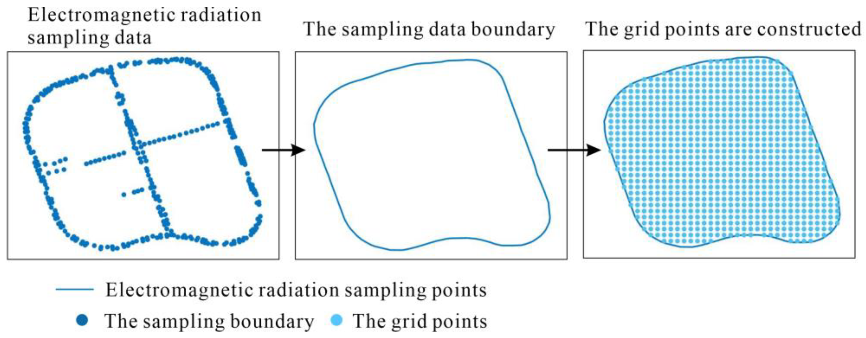
Before the LRBF method is used, the grid points are constructed within the sampling range. The sampling data boundary is first obtained. Then, the grid points with a certain interval distance are constructed within the boundary range (Figure 2).
In the process of constructing grid points, the accuracy of constructing an EMR-SF based on the LRBF is affected by the density of grid points. Finding the appropriate grid point interval distance effectively improves the interpolation accuracy of the LRBF. In this paper, a method is proposed to obtain the grid point interval distance, which calculates the maximum influence distance of the sample points based on the Gaussian basis function and then obtains the density of the grid points according to the maximum impact distance.

2.2.1. Maximum Influence Distance of the Sample Points

The value of the Gaussian basis function φ ( x x i ) in Equation (1) will affect the result of F(x), which can be expressed as:
φ ( x x i ) = e ε 2 x x i 2 0 x x i L 0     x x i L
where x represents the grid points, and xi is the sample points. x x i is the distance from the grid points to the sample points. L represents the maximum influence distance of the sample points; that is, when the distance from the grid points to the sample points is greater than L, the value φ ( x x i ) tends to zero, and the grid points are almost unaffected by the sample points.
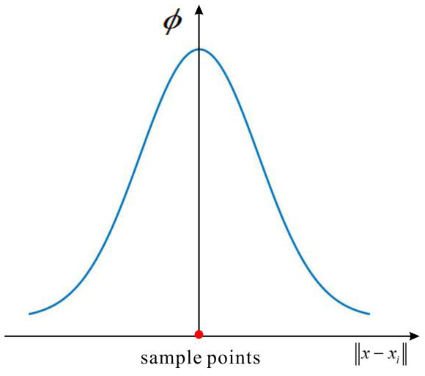
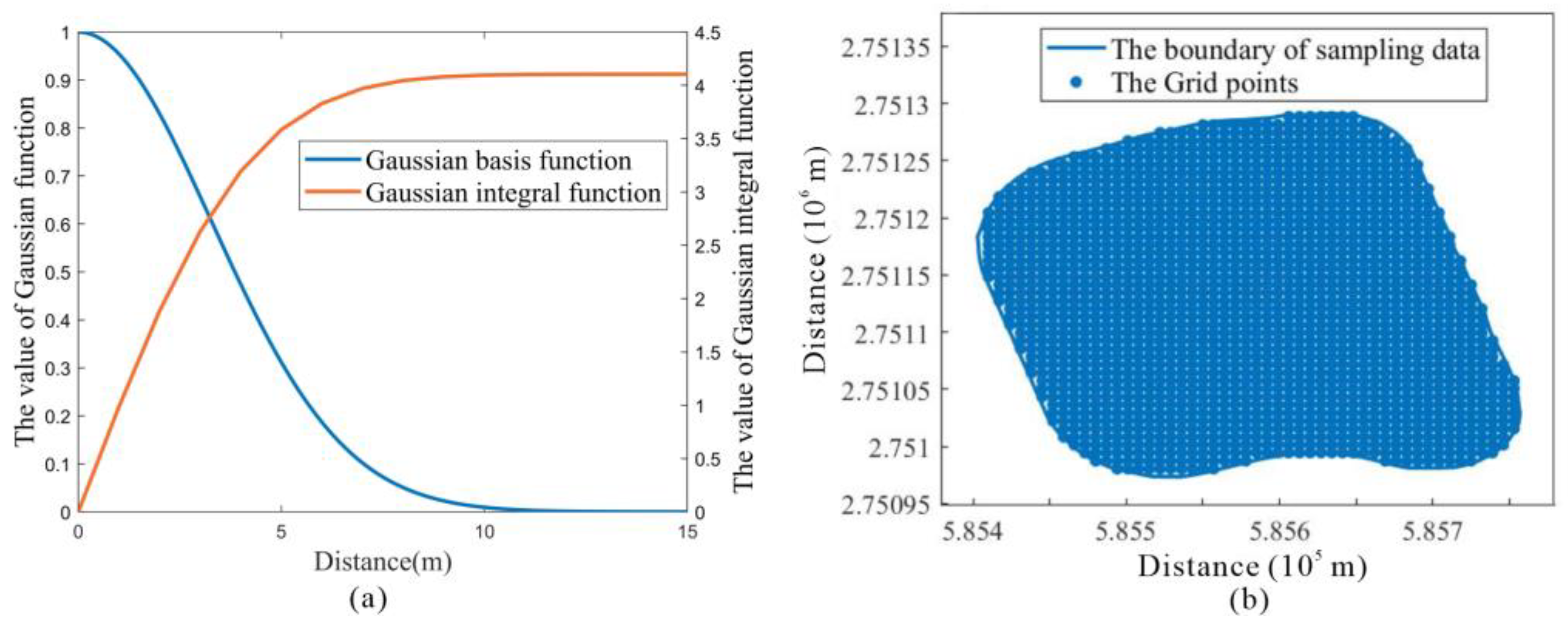
As the distance from the grid point to the sample point increases, the value of the Gaussian function decreases (Figure 3). When the distance increases to a certain value, the value of the Gaussian basis function is almost unchanged, and this value is used as the maximum influence distance L. The maximum influence distance L can be obtained by integrating the Gaussian basis function. The integral formula of the Gaussian basis function is:
F ( d ) = 0 d e ε 2 r 2 d r
where F(d) is the integral value of the Gaussian basis function from 0 to d, and d is the upper bound of the integral. ε is the shape parameter of the Gaussian basis function.

2.2.2. Grid Points Density

To ensure that the grid points can be influenced by the generation of the sample points, the distance between the sample points and the grid points should be within the maximum influence distance L. P1 and P2 are two sample points (Figure 4b). Two circles are made with the center of the two sample points and the radius of the maximum influence distance L. The range where two circles intersect is the area commonly affected by two sampling points, and the points within the range are affected by the two sample points. Considering that LRBF is an isotropic interpolation method, the grid point is required to be equally and most affected by the two sample points, so the location of the grid point is at the center of the two sample points, that is, at the position of L/2. Therefore, L/2 is used as the grid point separation distance, which is set to the density of the grid points to construct the grid points.

2.3. The Layered Grid Points in the LRBF

In the LRBF method, the layered interpolation after layering the grid points enables the EMR sample point data to interact with each other. This ensures that the EMR intensities of points close to each other are similar. Usually, similar points will show aggregation in space. If the points are aggregated to a high degree in a certain distance scale range, it means that there are many aggregated points. A distance scale that makes the maximum aggregation degree is found, based on which the stratification of the grid points can ensure that more similar points are aggregated and improve the interpolation accuracy of LRBF.
Ripley’s K function counts the number of points according to the search distance range of a certain radius, which is a point density distance function [26]. It can obtain the degree of aggregation of spatial data at different distance scales. The distance range corresponding to the maximum degree of aggregation of the sampled data can be obtained by using this function. This distance range is used as the stratified interval distance of LRBF. Ripley’s K function is defined as:
K ( d ) = A i = 1 n j = 1 n I ( d ) n ( n 1 )
I ( d ) = 1 , i f   r i j < d 0 , i f   r i j d
where d is the distance scale, A is the area of the study area, and n is the number of EMR sampling points. I is the number of EMR sampling points in the range of the distance scale d, and rij is the distance between the ith point and the jth point.
L ( d ) = K ( d ) π d
Assuming that the sample points are completely spatially random distributions, the expectation of L(d) is 0. When L(d) is less than 0, the EMR sampling data are discretely distributed. When L(d) is greater than 0, the EMR sampling data have an aggregated distribution. The distance scale d corresponds to the largest value of L(d) as the maximum aggregation distance, which represents the maximum spatial aggregation intensity of the EMR sampling data.
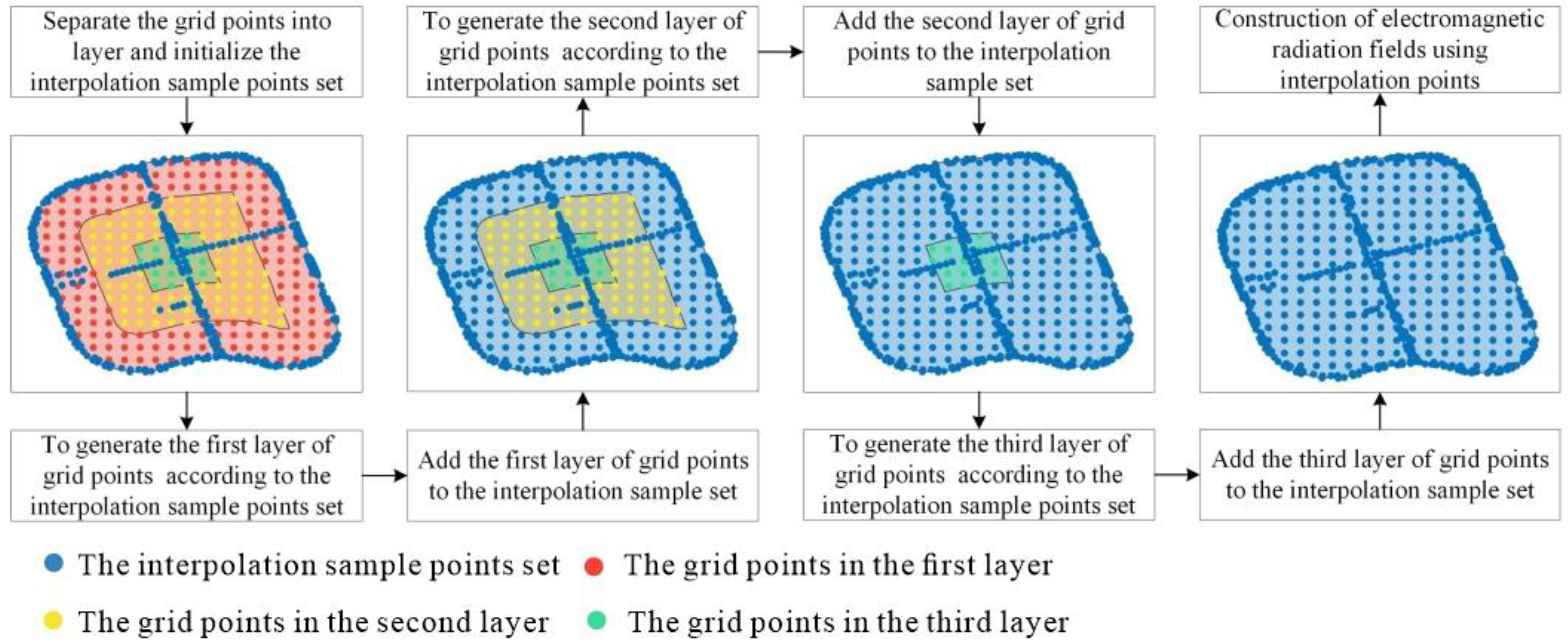
The maximum aggregation distance d is taken as the layered interval distance of the LRBF. The boundary line of the EMR sampling data is taken as the standard, and the interval distance H is used to gradually divide the grid points into multiple layers inward (Figure 5).

2.4. Construction of EMR-SF by the LRBF

The EMR data collected along the road are taken as the sample point set: S0 = {s1 (x1,y1,e1), s2 (x2,y2,e2),…, sn (xn,yn,en)}. The set of interpolated sample points is S. The set of grid points after stratification is G = {G1, G2,…, Gl}, where Gl= {g1 (x1,y1,ge1), g2 (x2,y2,ge2),…, gk (xk,yk,gek)}, representing the grid point at the layer l and so on. The process of constructing the EMR-SF using the LRBF spatial interpolation method is as follows:
(1)
The interpolation sample point set S = S0 is initialized, and the index number l = 1 is set.
(2)
Point set Gl is taken from the grid point set.
(3)
The EMR value of each point in point set Gl is generated by sample point set S according to Equation (1).
(4)
Point set Gl is added to the interpolation sample point set S to form a new interpolation sample point set S = S ∪ Gl.
(5)
l = l + 1.
(6)
Steps (2)–(5) are repeated until the EMR value of each grid point is calculated.
(7)
Finally, the EMR-SF is constructed according to the updated interpolation dataset S = {S0, G1, G2,..., Gl}.
The LRBF spatial interpolation method flow is shown in Figure 6:

3. Study Area and Data Collection

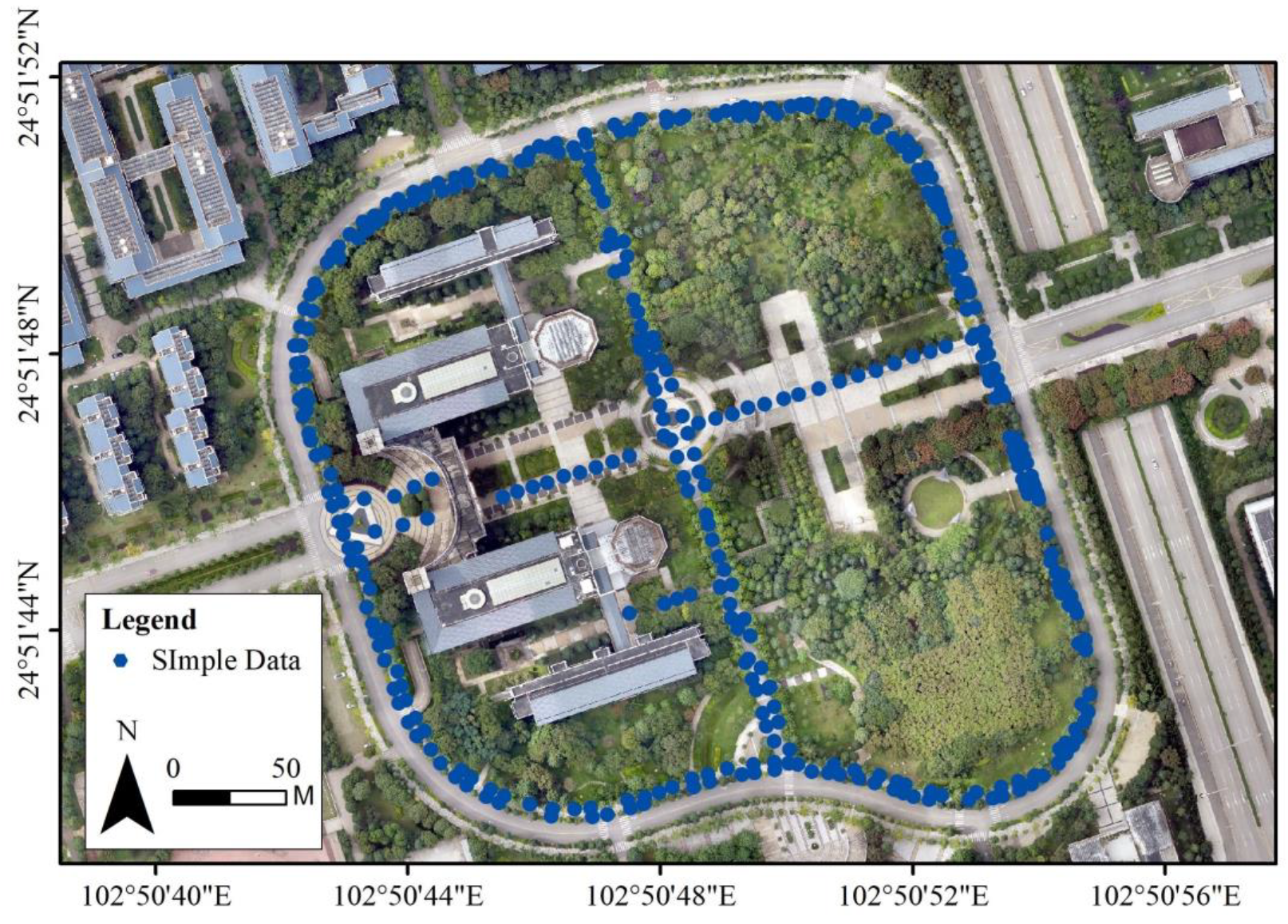
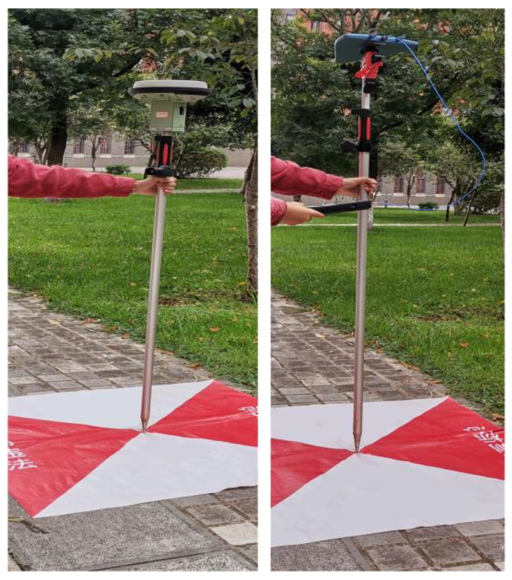
The campus of Yunnan Normal University in Kunming, China, is used as the study area, which is located between 24°51′42″ N–24°51′52″ N and 102°50′42″ E–102°50′56″ W. Half of the study area is covered by buildings, and the other half is covered by wood (Figure 7). The EMR can be analyzed under different environmental conditions. There are three major mobile communication base stations within the study area, and there are five places around the study area where mobile communication base stations exist (Figure 8). A handheld electromagnetic radiation detector HF-60105 is used to measure the EMR value in the environment, and the frequency range of this device is 9 khz–9.4 Ghz. The radiation frequency of the mobile communication base stations on campus is usually between 1710 and 1920 Mhz. To cover this frequency range and measure the electromagnetic radiation of mobile communication base stations, 1800 Mhz is selected as the center frequency, and the frequency range width is 400 Mhz for measurement. First, the global navigation satellite system (GNSS) receiver is used to obtain the corresponding coordinate information at each point, and the coordinate system is based on the China Geodetic Coordinate System 2000 (CGCS2000): measure the electromagnetic radiation value at a height of 1.5 m, set the measurement unit of the instrument to v/m and the sampling time to 30 min, and then measure the electromagnetic radiation value at each point (Figure 9). A total of 367 data measurements were collected, and each piece of data contains coordinate information and EMR values, and the EMR values were between 0.01 and 0.73 v/m.

4. Experimental Results

4.1. The Grid Point Construction Results in LRBF

The process of solving the maximum influence distance L using Gaussian basis function integration is as follows: (1) the initial value of d and the step size are set; (2) the value of F(d) and the value of F ( d + Δ d ) are calculated; (3) F ( d + Δ d ) F ( d ) and d = d + Δ d are calculated, if F ( d + Δ d ) F ( d ) < 0.001 , and the value of d is outputted; otherwise, Steps (2)–(3) are repeated. The final d is the maximum influence distance L (Figure 10).
In the LRBF method, the regular grid points are generated within the study area first. Based on the original EMR sampling data, the optimal shape parameters of the Gaussian basis function are calculated using PSO as ε = 0.2159 , and the Gaussian basis function expression is e 0.2159 2 x 2 . The Gaussian basis function is integrated using Equation (5), setting d = 0 and the step size Δ d = 1 . When the difference in the integration values between adjacent steps is less than 0.001, the maximum influence distance L = 14 m is obtained, and the Gaussian basis function and the integral function image are shown (Figure 11a). The interval of the grid points is set as L/2, which is 7 m, and the result of the LRBF grid opinion construction is shown (Figure 11b).

4.2. The Grid Points Layered Results in LRBF

After constructing the regular grid network, the grid points are separated into layers. Ripley’s K function is used to analyze the spatial distribution characteristics of the original EMR sampling data (Figure 12a). When the distance is between 0 and 75 m, the L(d) value of the EMR sampling data is greater than 0, and the EMR sampling data are spatially aggregated. After 75 m, the L(d) value of the EMR sampling data is less than 0, and the EMR sampling data are discrete in space. When the distance is 25 m, the L(d) value is the largest, and the EMR sampling data are aggregated to the largest degree. Therefore, the layered interval distance is set to 25 m, starting from the sampling data boundary and layering the grid points inward. The results of the layered grid points are shown (Figure 12b).

4.3. The EMR-SF Construction Results by LRBF

4.3.1. Experimental Results

The EMR-SF constructed using LRBF is shown (Figure 13). The EMR-SF constructed by LRBF is similar to a sector, which is one of the regions of the EMR-SF constructed based on the electromagnetic radiation propagation model with a strong radiation source as the center of the circle.
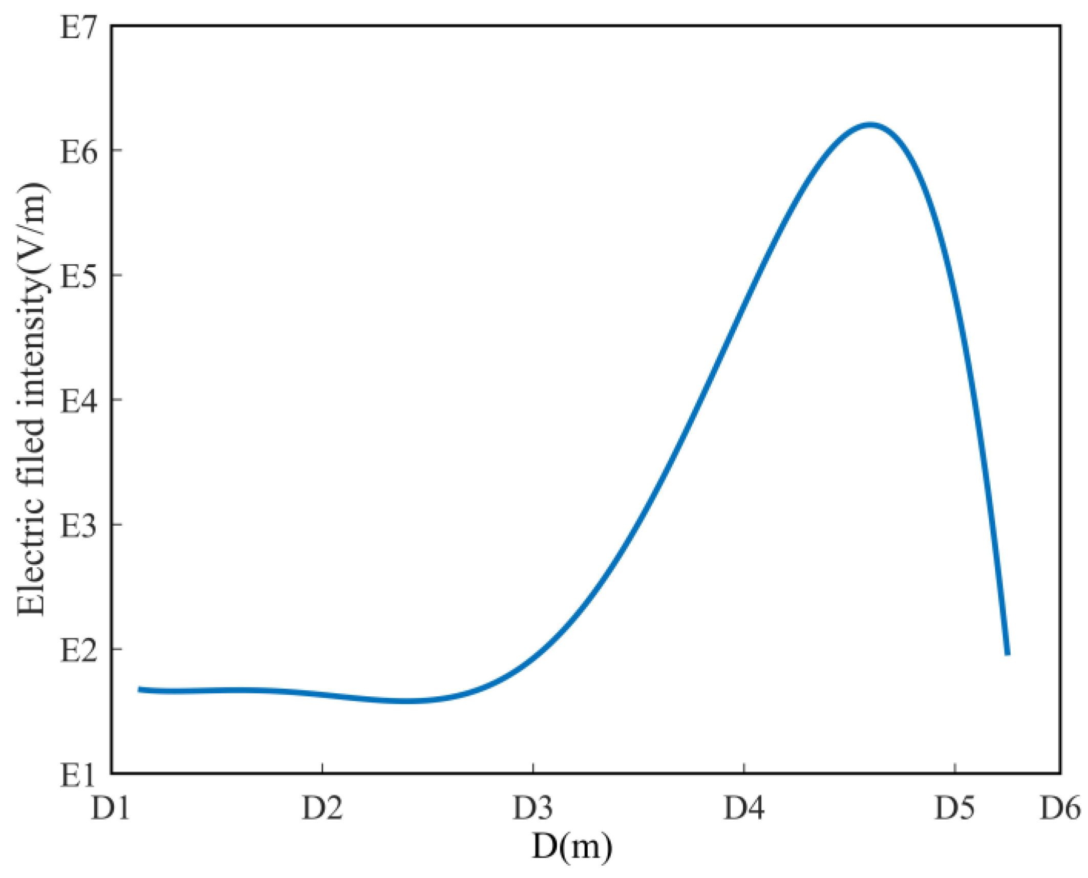
Without considering the EMR bypassing and reflection, the EMR intensity value is almost the same when the distance between the measurement position and the radiation source is the same. Usually, the EMR value at a position closer to the transmitting antenna is changed little and is enhanced after a certain distance. The EMR value begins to decrease after reaching the peak [27,28,29] (Figure 14). Therefore, the EMR value is weak at the place close to the mobile base station location, and the EMR value is enhanced at a place far from the mobile base station location.
Although there are mobile base station transmitting antennas on Teaching Building 1 and Teaching Building 2, the EMR value around them is not affected by them and is affected by the transmitting antenna of Teaching Building 4 (Figure 15). The transmitting antennas are on Dormitory Building 1, Dormitory Building 2, and Dormitory Building 3 (Figure 15); although they exist, they face the dormitory building area instead of the teaching building area. Generally, there exists a main transmitting direction for the transmitting antennas, and the radiation obtained in other directions is much smaller than the main transmitting direction. In this study area, the EMR mainly originates from the transmitting antennas in the northeast direction of Teaching Building 4 and Teaching Building 3, which causes the established EMR-SF to appear in the form of concentric sectors.

4.3.2. Accuracy Comparison

To verify the accuracy of the LRBF spatial interpolation method, the LRBF spatial interpolation method is compared with the IDW and OK methods. In this paper, the root mean square error (RMSE), mean absolute error (MAE), maximum error (MAXE), and minimum error (MINE) of the sampled data are calculated by the leave-one-out cross validation (LOOCV) method, which is used to evaluate the interpolation accuracy, and the calculated expressions are shown in Equations (7)–(10).
R M S E = 1 m m = 1 m [ f ( x ) f ( x ) ] 2
M A E = 1 m f ( x ) f ( x )
M A X E = max f ( x ) f ( x )
M I N E = min f ( x ) f ( x )
where m is the number of sampled data, f(x)′ is the EMR value of the sampled data calculated using the LRBF method, and f(x) is the real EMR value of the sampled data.
In the interpolation process, IDW and OK select 12 known points closest to the unknown point to calculate the EMR of the unknown point. The distance power of the IDW interpolation method is 2. The OK method uses a Gaussian function semi-variance model for fitting.
The error statistics of each interpolation method are shown (Table 1). The accuracy of IDW and OK are comparable. The IDW uses the distance between unknown points and sample points as the weighted average, which is more suitable for use in the case of a uniform distribution of sampled data. The OK mainly relies on the spatial autocorrelation of the data, which requires a sufficient number of sample points with strong spatial autocorrelation to produce a better interpolation accuracy. The main reason for the comparable interpolation accuracy of the IDW and OK is that the data collected along the road are linearly distributed, and the contribution of the sample points obtained by the two methods within a certain search field is not much different. This leads to the weight proportion coefficients of the two not being much different, which results in similar interpolation results for both.
In general, LRBF has a higher accuracy than the other two methods. The LRBF improves the approximation ability of RBF by increasing the sample points of RBF interpolation. At the same time, sample points are only added within a certain distance to ensure the shape characteristics of the RBF basis function. This improves the stability of the constructed surface function and thus improves the interpolation accuracy of LEBF.
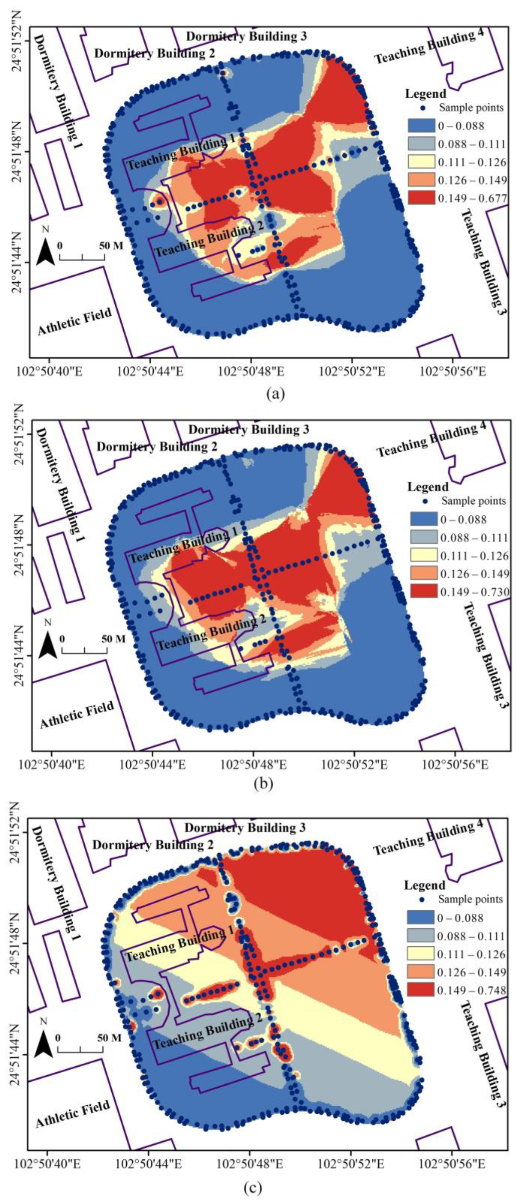
The results of the EMR-SF constructed by different interpolation methods are shown (Figure 16). IDW and OK construct the EMR-SF using sample points within a certain search range. However, the EMR data collected along the road have a large range of blank areas overall, and they are linearly distributed locally. It is easy to conclude that the EMR intensity generated by IDW and OK in a certain range is the same. For example, IDW and OK only refer to the sample points on the main road for the EMR value on the north side of Teaching Building 1, so the EMR value they generate is in the same range as the value on the main road. However, the EMR value increases and then decreases within a certain distance from the transmitting antenna, and there is an obvious zoning phenomenon (Figure 11). Thus, the accuracy of constructing the EMR-SF of IDW and OK is low. While the EMR-SF constructed by LRBF is more in line with the EMR-SF constructed by the propagation characteristics of EMR, the construction accuracy of LRBF is higher than that of IDW and OK.

5. Discussion

In this chapter, the necessity of regular grid points constructed and layered interpolation in LRBF is discussed. Meanwhile, the applicability of the methods involved in LRBF regarding the acquisition of the grid point interval distance and the acquisition of the layered interval distance is examined.

5.1. Grid Point Constructed and Layered Interpolation

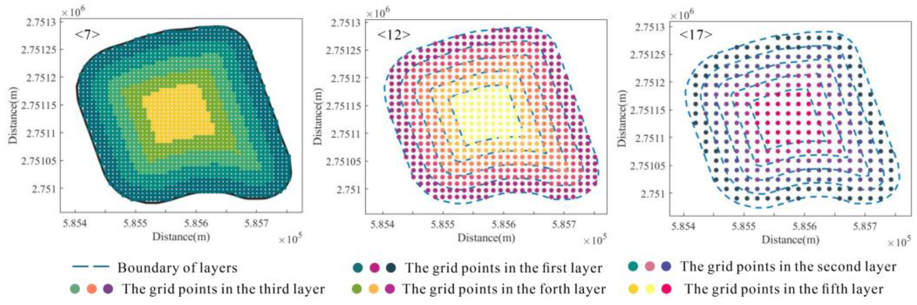
To further understand the advantages of adding grid points and layered interpolation, the LRBF spatial interpolation method was compared with the RBF with the grid points (RBFGP) method, which only adds grid points without layered interpolation. The interval distances of the grid points are 7 m, 12 m, and 17 m (Figure 17), respectively. The root mean square error statistics of each method with different interval densities are shown (Table 2).
In summary (Table 2), the accuracy of LRBF is higher than that of RBFGP for the same grid interval distance after a layered approach that improves the interpolation accuracy of RBF. Compared with generating all the grid points at once, the layered interpolation that generates the grid points allows RBF to ensure the approximation of the basis function in the close range in the local range.

5.2. Comparison of the Result of EMR-SF between Different Interval Distances of the Grid Point by LRBF

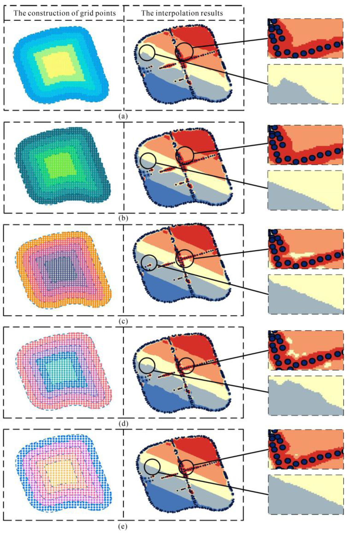
In this section, the applicability of the grid point interval distance acquisition method provided in this paper will be discussed. The maximum impact distance is compared with other grid interval distances, the layered interval distance of the LRBF is 25 m, and their error statistics are shown (Table 3).
The accuracy of LRBF increases gradually as the distance between the grid points decreases. The accuracy of LRBF is improved substantially when the grid point interval distance reaches a certain level, but it does not improve the interpolation accuracy by decreasing the interval distance of the grid point all the time. Compared with the interval distance of 7 m, the accuracy of the interval distance of 6 m in LRBF does not improve significantly. At the same time, the time cost increases significantly as the interval distance of the grid points decreases.
The EMR-RF constructed by the LRBF at different interval distances of grid points is shown (Figure 18). When the interval distances of grid points are 6 m, 8 m, 9 m, and 10 m, the EMR-SF construction is not sufficiently smooth, and the EMR-SF constructed by them in the central region shows obvious discontinuities. The EMR-SF constructed by using LRBF with the maximum influence distance (grid point interval distance is 7 m) is smoother compared with others, and the space field grading is more obvious.
In the LRBF interpolation method, each added grid point is derived from the value of the sampling point, and the distance between the grid points will also affect the degree of influence of the sampling point on the grid point. When the distance between grid points is too large, such as 10 m or 9 m, the influence of sampling points on grid points is weakened, and the interpolation accuracy of LRBF is very low. It is important to choose the optimal grid point interval distance for LRBF. The Gaussian function is used to obtain the maximum influence distance of the sampling data, and the interaction between point pairs is considered. Half of the maximum influence distance is used as the grid point interval distance, and the influence of the sampling point on the grid point is considered. This can quickly obtain the grid point interval distance, and the comparison of the results shows that setting the grid point spacing distance according to the maximum influence distance can improve the construction accuracy of the EMR-SF by LRBF.

5.3. Comparison of the Result of EMR-SF between Different Layered Interval Distances by LRBF

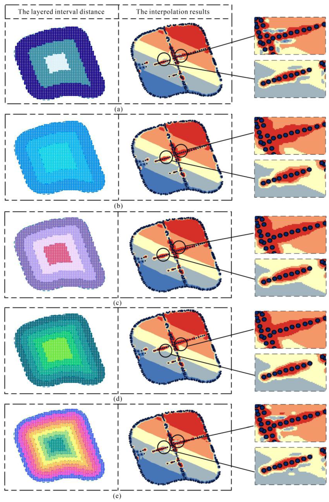
In this section, the applicability of the layered interval distance of the grid point acquisition method provided in this paper will be discussed. The maximum aggregation distance and the layered interval distances of 55 m, 45 m, 35 m, 25 m, and 15 m are used as a comparison. The interval distance of the grid points of LRBF is set to 7 m. The error statistics for the LRBF with different layered interval distances are shown (Table 4).
The accuracy of LRBF with different layered interval distances varies (Table 4). In general, the accuracy of LRBF gradually improves as the layered interval distance decreases, but it is not better as the layered interval distance decreases. When the layered interval distance is 15, the accuracy is lower than that when the layered interval distances are 35 m and 25 m. The EMR-SF constructed by LRBF with different layering interval distances is shown (Figure 19). When the layered interval distances are 55 and 15, the electromagnetic field constructed in the central region appears to be less reasonable, and the space field obviously appears to be discontinuous. This indicates that an interval distance that is too large or too small is not conducive to the construction of the EMR-SF used by LRBF. The EMR-SF is similar for 45-, 35-, and 25-layered interval distances; finally, they have similar accuracy in the interpolation error.
The construction accuracy and visualization results of the EMR-SF show that the LRBF obtains a large error if the layered interval distance is too large or too small. A too-small layered interval distance will increase the number of layers, thereby increasing the amount of calculation and causing excessive error transmission. To obtain a better layered interval distance, from the view of the distribution pattern of sampling points, the maximum aggregation distance was calculated by using Ripley’s K function to be 25 m. Taking this distance as the LRBF layer interval distance, and comparing the error with other values, it can be seen that this method of obtaining the layer interval distance based on the distribution pattern of sampling points improves the construction accuracy of EMR-SF by LRBF.

6. Conclusions

The EMR data collected along the road are spatially distributed in a line shape. These data are unevenly distributed, and there is an empty region in the center of the data-sampling area. The accuracy of generating the EMR-SF using the RBF interpolation method is low under such data distribution. To address this problem, the LRBF spatial interpolation method is proposed for the construction of EMR-RF data collected along roads. In this method, a certain density of grid points is constructed in advance in the empty region of the study area, which can be used to increase the number of sample points in LRBF so that LRBF can obtain stable sample points in the empty region. Then, the grid points are separated into multiple layers from outside to inside. Finally, the LRBF spatial interpolation method is used to generate the EMR values of the grid points in layers. This can enable the LRBF basis function to ensure a certain shape in the local range and improve the LRBF interpolation accuracy to construct a better EMR-SF.
The electromagnetic data detected along the road in the study area are collected by the EMR instrument, and the EMR-SF within the study area is constructed according to the LRBF. The experimental results show that when the number of electromagnetic radiation data samples along the road is small, the EMR-SF constructed by LRBF is better than the classical spatial interpolation methods, such as the IDW and OK methods, in terms of precision and visualization. It obtains a more accurate and continuous EMR-SF. In addition, the construction accuracy of the EMR-SF by LRBF under different grid point interval distances and layered interval distances is also discussed. According to the maximum influence distance and the maximum aggregation distance obtained from the distribution pattern of sampling points to set the LRBF grid point and layered interval distance, the accuracy of the construction of EMR-SF by LRBF is improved.

Author Contributions

J.Z. wrote the paper and did the experiment. P.D. proposed the method of the whole paper. J.L. (Jia Li) verified the accuracy of the experiment. J.L. (Jiajia Liu) collected experimental data. All authors have read and agreed to the published version of the manuscript.

Funding

This research was funded by the National Natural Science Foundation of China [41901336], the Yunnan Fundamental Research Projects [202101AT070078], the ‘Revitalizing Yunnan Talents Support Program’ project [YNWR-QNBJ-2020-103], and the Yunnan Academician and Expert Workstation [2017IC063] funding support.

Institutional Review Board Statement

Not applicable.

Informed Consent Statement

Not applicable.

Data Availability Statement

The data that support the findings of this study are openly available in ‘figshare.com’ at https://doi.org/10.6084/m9.figshare.21679379.v1 (accessed on 6 December 2022).

Conflicts of Interest

The authors declare no conflict of interest.

References

  1. Sagnard, F. Educational Graphical Interfaces to Learn about Radiation and Propagation of Electromagnetic Waves. IEEE Trans. Educ. 2004, 47, 389–396. [Google Scholar] [CrossRef]
  2. Redlarski, G.; Lewczuk, B.; Żak, A.; Koncicki, A.; Krawczuk, M.; Piechocki, J.; Jakubiuk, K.; Tojza, P.; Jaworski, J.; Ambroziak, D. The Influence of Electromagnetic Pollution on Living Organisms: Historical Trends and Forecasting Changes. BioMed Res. Int. 2015, 2015, 234098. [Google Scholar] [CrossRef] [PubMed] [Green Version]
  3. Sarkar, T.K.; Abdallah, M.N.; Salazar-Palma, M. Survey of Available Experimental Data of Radio Wave Propagation for Wireless Transmission. IEEE Trans. Antennas Propag. 2018, 66, 6665–6672. [Google Scholar] [CrossRef]
  4. Mollel, M.S.; Michael, K. Comparison of Empirical Propagation Path Loss Models for Mobile Communication. 2014. Available online: https://dspace.nm-aist.ac.tz/handle/20.500.12479/1167 (accessed on 4 May 2021).
  5. Yilmaz, H.B.; Tugcu, T. Location estimation-based radio environment map construction in fading channels. Wirel. Commun. Mob. Comput. 2015, 15, 561–570. [Google Scholar] [CrossRef]
  6. Oudira, H.; Diouane, L.; Garah, M. Empirical Path Loss Models Optimization for Mobile Communication. In Proceedings of the 2018 IEEE 5th International Congress on Information Science and Technology (CiSt), Marrakech, Morocco, 21–27 October 2018; pp. 443–448. [Google Scholar]
  7. Faruk, N.; Popoola, S.I.; Surajudeen-Bakinde, N.T.; Oloyede, A.A.; Abdulkarim, A.; Olawoyin, L.A.; Ali, M.; Calafate, C.T.; Atayero, A.A. Path Loss Predictions in the VHF and UHF Bands within Urban Environments: Experimental Investigation of Empirical, Heuristics and Geospatial Models. IEEE Access 2019, 7, 77293–77307. [Google Scholar] [CrossRef]
  8. Maiti, P.; Mitra, D. Complexity reduction of ordinary kriging algorithm for 3D REM design. Phys. Commun. 2022, 55, 101912. [Google Scholar] [CrossRef]
  9. Navarro-Camba, E.A.; Segura-García, J.; Gomez-Perretta, C. Exposure to 50 Hz Magnetic Fields in Homes and Areas Surrounding Urban Transformer Stations in Silla (Spain): Environmental Impact Assessment. Sustainability 2018, 10, 2641. [Google Scholar] [CrossRef] [Green Version]
  10. Céspedes, V.H.; Cadavid, L.F.D.; Gómez, Y.A.G. Electromagnetic pollution maps as a resource for assessing the risk of emissions from mobile communications antennas. Int. J. Electr. Comput. Eng. 2020, 10, 4244–4251. [Google Scholar] [CrossRef]
  11. Tuysuz, B.; Mahmutoglu, Y. Measurement and mapping of the GSM-based electromagnetic pollution in the Black Sea region of Turkey. Electromagn. Biol. Med. 2017, 36, 132–140. [Google Scholar] [CrossRef]
  12. Li, Z. An enhanced dual IDW method for high-quality geospatial interpolation. Sci. Rep. 2021, 11, 9903–9917. [Google Scholar] [CrossRef]
  13. Zhao, W.; Cao, T.; Li, Z.; Sheng, J. Comparison of IDW, cokriging and ARMA for predicting spatiotemporal variability of soil salinity in a gravel–sand mulched jujube orchard. Environ. Monit. Assess. 2019, 191, 376. [Google Scholar] [CrossRef]
  14. Gu, K.; Zhou, Y.; Sun, H.; Dong, F.; Zhao, L. Spatial distribution and determinants of PM2. 5 in China’s cities: Fresh evidence from IDW and GWR. Environ. Monit. Assess. 2021, 193, 15. [Google Scholar] [CrossRef]
  15. Han, Z.; Liao, J.; Qi, Q.; Sun, H.; Wang, J. Radio Environment Map Construction by Kriging Algorithm Based on Mobile Crowd Sensing. Wirel. Commun. Mob. Comput. 2019, 2019, 4064201. [Google Scholar] [CrossRef] [Green Version]
  16. Uddin, M. On the selection of a good value of shape parameter in solving time-dependent partial differential equations using RBF approximation method. Appl. Math. Model. 2014, 38, 135–144. [Google Scholar] [CrossRef]
  17. Casciola, G.; Lazzaro, D.; Montefusco, L.B.; Morigi, S. Shape preserving surface reconstruction using locally anisotropic radial basis function interpolants. Comput. Math. Appl. 2006, 51, 1185–1198. [Google Scholar] [CrossRef] [Green Version]
  18. Casciola, G.; Montefusco, L.B.; Morigi, S. Edge-driven Image Interpolation using Adaptive Anisotropic Radial Basis Functions. J. Math. Imaging Vis. 2010, 36, 125–139. [Google Scholar] [CrossRef]
  19. Casciola, G.; Lazzaro, D.; Montefusco, L.B.; Morigi, S. Fast surface reconstruction and hole filling using positive definite radial basis functions. Numer. Algorithms 2005, 39, 289–305. [Google Scholar] [CrossRef]
  20. Buhmann, M.D. Radial Basis Functions: Theory and Implementations; Cambridge University Press: Cambridge, UK, 2003; Volume 12. [Google Scholar]
  21. Fornberg, B.; Zuev, J. The Runge phenomenon and spatially variable shape parameters in RBF interpolation. Comput. Math. Appl. 2007, 54, 379–398. [Google Scholar] [CrossRef] [Green Version]
  22. Fasshauer, G.E.; Zhang, J.G. On choosing “optimal” shape parameters for RBF approximation. Numer. Algorithms 2007, 45, 345–368. [Google Scholar] [CrossRef]
  23. Bayona, V.; Moscoso, M.; Kindelan, M. Optimal constant shape parameter for multiquadric based RBF-FD method. J. Comput. Phys. 2011, 230, 7384–7399. [Google Scholar] [CrossRef]
  24. Kennedy, J.; Eberhart, R. Particle swarm optimization. In Proceedings of the ICNN’95—International Conference on Neural Networks, Perth, WA, Australia, 27 November–1 December 1995; pp. 11–23. [Google Scholar] [CrossRef]
  25. Abualigah, L.M.; Khader, A.T.; Hanandeh, E.S. A new feature selection method to improve the document clustering using particle swarm optimization algorithm. J. Comput. Sci. 2018, 25, 456–466. [Google Scholar] [CrossRef]
  26. Hohl, A.; Zheng, M.; Tang, W.; Delmelle, E.; Casas, I. Spatiotemporal point pattern analysis using Ripley’s K function. In Geospatial Data Science Techniques and Applications; CRC Press: Boca Raton, FL, USA, 2017; pp. 155–176. [Google Scholar]
  27. Coco, S.; Laudani, A.; Mazzurco, L. A novel 2-D ray tracing procedure for the localization of EM field sources in urban environment. IEEE Trans. Magn. 2004, 40, 1132–1135. [Google Scholar] [CrossRef]
  28. Zvezdina, M.Y.; Shokova, Y.A.; Krivtsova, M.; Saldaev, D.; Shashkin, O. Electromagnetic environment estimation near communications system reflector antennae. In Proceedings of the 2017 Radiation and Scattering of Electromagnetic Waves (RSEMW), Divnomorskoe, Russia, 26–30 June 2017; pp. 69–72. [Google Scholar]
  29. Zvezdina, M.Y.; Shokova, Y.A.; Kundryukova, N.; Kutukova, V.; Pozdnyakova, A. Visualization of electromagnetic environment near GSM antennae. IOP Conf. Ser. Earth Environ. Sci. 2017, 50, 012029. [Google Scholar] [CrossRef] [Green Version]
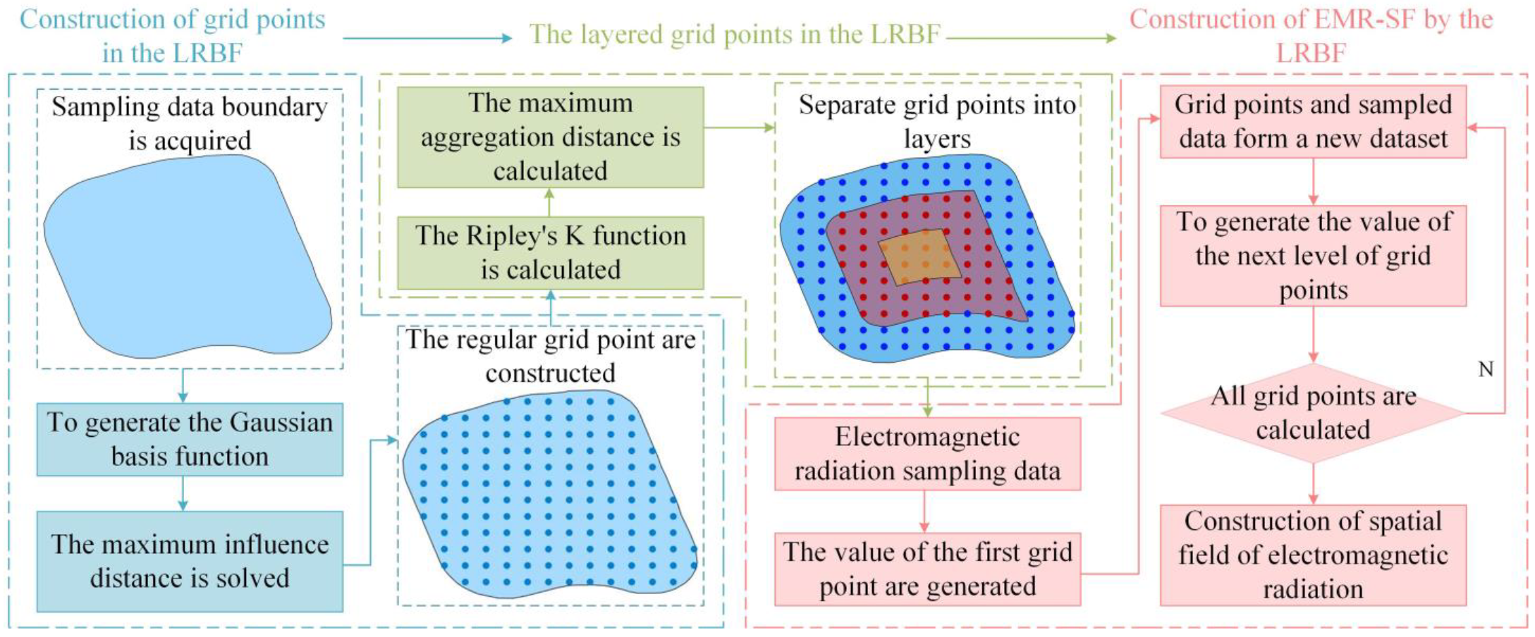
Figure 1. Construction of the EMR-SF by LRBF.
Applsci 13 06153 g001
Figure 2. Grid point construction.
Applsci 13 06153 g002
Figure 3. Gaussian basis function.
Applsci 13 06153 g003
Figure 4. The influence range of the Gaussian basis function: (a) the 3D Gaussian basis function; (b) 3D top view of the Gaussian basis function.
Applsci 13 06153 g004
Figure 5. Grid point layered. (a) The grid points. (b) The first layer. (c) The second layer. (d) The third layer.
Applsci 13 06153 g005
Figure 6. Procedure of the EMR-SF construction by LRBF.
Applsci 13 06153 g006
Figure 7. The study area.
Applsci 13 06153 g007
Figure 8. Various types of EMR base stations.
Applsci 13 06153 g008
Figure 9. Coordinate acquisition of sampled data.
Applsci 13 06153 g009
Figure 10. Maximum influence distance solution procedure.
Applsci 13 06153 g010
Figure 11. Grid point construction results. (a) The Gaussian basis function and the integral function. (b) The result of construction of the grid points.
Applsci 13 06153 g011
Figure 12. Grid point layering results. (a) The L(d) value of the EMR sampling data. (b) The result of layered grid points.
Applsci 13 06153 g012
Figure 13. EMR-SF constructed by LRBF.
Applsci 13 06153 g013
Figure 14. The EMR intensity changing with the horizontal distance of the measuring point from the antenna.
Applsci 13 06153 g014
Figure 15. Mobile base station location and antenna pattern.
Applsci 13 06153 g015
Figure 16. Construction results of EMR-SF by different space field methods. (a) The interpolation results by IDW. (b) The interpolation results by OK. (c) Interpolation results by LRBF.
Applsci 13 06153 g016
Figure 17. Different interval distances of grid points.
Applsci 13 06153 g017
Figure 18. Comparison of LRBF with different interval distances of grid points. (a) The interval distance is 6. (b) The interval distance is 7. (c) The interval distance is 8. (d) The interval distance is 9. (e) The interval distance is 10.
Applsci 13 06153 g018
Figure 19. Comparison of LRBF with different layered interval distances. (a) The interval distance is 55. (b) The interval distance is 45. (c) The interval distance is 35. (d) The interval distance is 25. (e) The interval distance is 15.
Applsci 13 06153 g019
Table 1. Error of each interpolation method (v/m).
Interpolation MethodOrdinary KrigingIDWLRBF
RMSE0.05820.04820.0378
MAE0.02950.03230.0179
MAXE0.500.470.45
MINE0.8 × 10−50.2 × 10−40.3 × 10−4
Table 2. Error of different methods for different interval densities (v/m).
Interval Distance of Grid Point (m)RBFGPLRBF
170.07410.0713
120.06970.0645
70.04250.0378
Table 3. Error of different interval distances of grid points (v/m).
Interval Distance of Grid Points (m)RMSEMAEMAXEMINE
100.06180.03220.5080.2 × 10−5
90.05680.02920.5120.1 × 10−7
80.05680.02890.5240.1 × 10−4
7 (maximum influence distance)0.03780.01790.450.3 × 10−4
60.03560.02110.320.8 × 10−7
Table 4. Different layered interval errors (v/m).
Layered Interval Distance (m)RMSEMAEMAXEMINE
550.04530.02310.470.9 × 10−7
450.03980.02310.510.5 × 10−4
350.03730.01760.450.3 × 10−5
25 (maximum aggregation distance)0.03780.01790.450.2 × 10−4
150.04180.01950.430.3 × 10−4
Disclaimer/Publisher’s Note: The statements, opinions and data contained in all publications are solely those of the individual author(s) and contributor(s) and not of MDPI and/or the editor(s). MDPI and/or the editor(s) disclaim responsibility for any injury to people or property resulting from any ideas, methods, instructions or products referred to in the content.