1. Introduction
The marine aquaculture industry has experienced significant growth in recent decades, becoming a vital contributor to global food production. However, it also faces a variety of challenges, both natural and human-induced. As most aquaculture operations take place in the sea with little control over environmental conditions, the industry is susceptible to threats from changes such as reduced oxygen or extreme temperatures that affect the growth and survivability of farmed species and increased costs, events that are more frequent due to climate change [
1]. Greece is one of the main producers of European seabass (
Dicentrarchus labrax) and gilthead sea bream (
Sparus aurata) in Europe, representing over 60% of the total European production according to the FEAP [
2]. Greek aquaculture has a significant contribution to the national economy as it represents 65% of fish production and is expected to keep an annual mean growth rate of 7% by 2030 according to the annual report of the Federation of Greek Maricultures (FGM) and the strategic development plan [
3]. Given this context, the promotion of sustainable development in the marine aquaculture industry is crucial, not only for Greece but also for the EU, as it is considered one of the key pillars of the Blue Growth strategy.
Apart from the interaction with coastal zone activities, aquaculture operations demand continuous and accurate monitoring. While in-situ data often present inconsistencies in terms of both quality and spatial coverage, remote sensing provides new opportunities for monitoring the ocean through frequent and cost-effective coverage of the entire Earth’s surface, even in remote locations. The Sentinel satellite missions are a part of the European Earth Observation Program “Copernicus”, which offers free data in various spectral regions (radar, optical, infrared) and at various spatial resolutions. The Sentinel missions, along with the CMEMS (Copernicus Marine Environmental Monitoring Service) digital repository, provide data on the oceans through advanced instruments and models, with a wide range of spatial and temporal resolutions. The combination of these data can provide valuable information on the quality of the environment in aquaculture areas.
The rapid growth of aquaculture and the continuous pressure the industry faces nowadays are leading to the relocation of facilities to offshore areas. This is carried out in order to minimize the negative impacts to the coastal zone; however, it brings along various challenges and difficulties. To mitigate the challenges and to improve the current practice towards a more sustainable aquaculture sector, researchers have increasingly turned to “precision farming” techniques to develop new, innovative methods and tools for monitoring and managing farm operations. The “precision farming” approach, which is already well established in land-based farming and has yielded positive results, aims to improve the sustainability of marine farming by reducing costs, increasing data accuracy, and reducing the reliance on human labor [
4].
Marine farming, however, presents its own set of difficulties due to the complex nature of the environment, the diversity of species being farmed, and exposure to external threats. Despite the abovementioned challenges, the concept of “precision fish farming” has garnered significant attention among researchers, leading to the development of new technologies and methods to improve monitoring and management of day-to-day operations [
4,
5,
6,
7,
8,
9,
10,
11]. Precision fish farming, as outlined by Føre et al. [
4], aims to apply control engineering principles in fish production to boost farm monitoring, control, and document biological processes. This approach allows commercial aquaculture to shift from a traditional, experience-based production method to a knowledge-based method that employs cutting-edge technologies and automated systems to tackle the challenges of aquaculture monitoring and management. The goal of precision fish farming is to improve the accuracy, precision, and repeatability of farming operations.
The significant expansion of aquaculture poses both risks and opportunities that require careful evaluation and appropriate measures for adaptation. Aquaculture procedures are complex due to the presence of numerous environmental drivers, such as temperature, extreme events, and harmful algal blooms, their interactions with production systems, and knowledge gaps about fish responses [
1,
12]. To support and facilitate decision making in this context, Decision Support Systems (DSSs) have been proposed as appropriate tools. DSSs are computer-based information systems designed to aid the decision-making process in complex situations, using data, models, and algorithms to generate insights and provide users with timely and accurate information to help them evaluate and compare alternative options. Typically, the decision-making process with a DSS involves several steps, including data gathering, analysis, and visualization, scenario analysis, and evaluation of alternatives. In addition, a DSS must provide decision makers with supporting information to enable strategic decisions for promoting industry sustainability in the coming decades. Furthermore, a DSS must achieve a balance between containing sufficient information and being user-friendly for accessibility [
13].
The goal of this study is to examine how satellite technology can assist in addressing the issues that arise from the rapid growth of fish farming. The main objectives are as follows: (a) to determine which parameters have an impact on aquaculture processes and how remote sensing can aid in their assessment, (b) to establish what indicators could be used as “warning signs” and their corresponding appropriate thresholds, and (c) to evaluate the system’s performance in real-life scenarios. This paper presents a web-based platform called “Aquasafe” which serves as a decision support system that constantly monitors fish farming operations and provides early warnings for potential risks. It combines satellite and in-situ data to give comprehensive insights and alerts to farm operators. The platform offers a combination of satellite data, in-situ measurements, and meteorological information, providing forecasts and alerts to aid in the effective management of fish farming operations. Ultimately, the system is intended to aid in the effective management of fish farming operations by providing valuable, accurate information about current conditions and production.
2. Materials and Methods
2.1. Overview of Aquasafe Structure
Aquasafe is a web-based platform created through a collaborative effort that brought together scientists and stakeholders. Aquasafe employs data from multiple sources to calculate important parameters, which are then utilized to derive indicators serving as warning signs for supporting aquaculture farm management. Aquasafe is structured into four main pillars: (a) input data, (b) estimated parameters, (c) indicators, and (d) web-based platform (
Figure 1).
- (a)
The input data, which include information from both satellites and
in-situ measurements, are used to determine the relevant parameters (
Figure 1a).
- (b)
The estimated parameters, which include water temperature, dissolved oxygen, chlorophyll-a, biogenic oil film, and fish growth metrics, are derived from the processing of the input data and are then combined to determine the indicators or “warning signs” (
Figure 1b).
- (c)
Five indicators based on the aforementioned parameters, namely algal blooms, sea surface temperature, saturation of dissolved oxygen, fish growth, and wind speed/gusts, were identified. These indicators are used to alert the administrator or operator of the farm of potential threats and required actions (
Figure 1c). All the indicators are a combination of two or more parameters, except for the sea surface temperature, which is used directly. More details on the combinations and the thresholds for the alerts are described in
Section 2.4.
- (d)
All of the elements described above are integrated and visualized into the Aquasafe web-based platform (
Figure 1d), providing forecasts and alerts to the administrator or operator of the farm.
2.2. Data
Aquasafe utilizes data from both satellites, models, and
in-situ measurements to acquire meteorological, physical, biochemical, and economic information about fish farms and their surrounding areas (
Figure 1a). The use of multiple data sources has the advantage of providing a more comprehensive view of the farming areas. Satellites provide multispectral, thermal, and SAR data, which are used to estimate several parameters.
In-situ measurements serve to validate the satellite estimations and provide additional information about the farmed species and their growth. Additionally, meteorological data such as winds, rainfalls, and cloud coverage, as well as data about extreme weather events, are also taken into consideration.
2.2.1. Satellite and CMEMS Data
The satellite data used in this study were obtained free of charge from the Copernicus services. Specifically, we utilized data from Sentinels 1, 2, and 3, as well as the Copernicus Marine Environment Monitoring Service (CMEMS). The input data sources and processing levels, as well as the available spatial and temporal resolution, are presented in
Table 1.
Sentinel-1 is a Synthetic Aperture Radar (SAR) mission of the Copernicus program, funded by the European Commission in partnership with the European Space Agency (ESA), which aims to provide data for ocean and land monitoring. The mission provides data regardless of weather and light conditions, as well as cloud coverage. The input data used in this study were Level-1 Ground Range Detected (GRD) products projected onto a ground range using an Earth ellipsoid model. These data were used for the detection of surface oils near fish farming sites. According to previous research, VV polarization offers a better clutter-to-noise ratio and is preferred for the detection of sea surface oils, which are indirectly detected as differences in sea surface roughness [
14,
15,
16,
17,
18].
Sentinel-2 mission is mainly designed as a land-monitoring mission but is widely used for coastal waters as well. Sentinel-2 twin satellites (Sentinel-2A and Sentinel-2B) are equipped with a multispectral sensor (Multispectral Imager—MSI, manufacturing led by Airbus Defence and Space, Friedrichshafen, Germany, developed and operated by European Space Agency) with 13 spectral bands at 10, 20, and 60 m of resolution covering the optical, near-infrared, and shortwave infrared part of the spectrum, thus providing high-resolution imagery with global coverage every 5 days (
https://sentinels.copernicus.eu/web/sentinel/missions/sentinel-2 (accessed on 20 April 2023)). Sentinel-2 data were used for the estimation of chlorophyll-a and dissolved oxygen, as well as for the detection of surface oils near the farms. Both Level-1C and Level-2A data were exploited, and they were georeferenced in WGS84/UTM automatic zone projection.
Sentinel-3 imagery was also found to be appropriate for such applications due to its spatial and temporal properties. Sentinel-3 is designed for ocean color applications specializing in estimating various Essential Oceanographic Variables (EOVs) on the surface layer (
https://sentinels.copernicus.eu/web/sentinel/missions/sentinel-3 (accessed on 20 April 2023)). Ocean color data are produced by the imagery acquired through the OLCI sensor with a spatial resolution of 300 m. OLCI’s products can be used to retrieve surface-level chlorophyl-a concentration, total suspended matter concentration, the light attenuation coefficient, and other EOVs. The satellites are also equipped with the SLSTR sensor, which is used for the SST estimation. The resolution of the datasets varies between the sensors with OLCI having 300 m spatial resolution products and SLSTR 1000 m. The footprint of the imagery ensures the coverage of large marine areas which in favorable days can contain the whole of the Greek seas. Furthermore, the temporal coverage of the mission is estimated between 1–2 days, enabling continuous monitoring of specific and wide marine regions.
The Copernicus Marine Environment Monitoring Service (CMEMS) provides regular and systematic biogeochemical and physical information on the marine environment. Within the context of our study, we utilized Level-4, daily, gap-free satellite observations for chlorophyll-a concentration and sea surface temperature from multi-platform observations. We used CMEMS data to describe environmental conditions and investigate their correlation with dissolved oxygen concentration (DO). By understanding this relationship,
in-situ observations of DO were used with our previously published work [
19] to train a machine learning regression model.
2.2.2. In-Situ
In-situ data are being used for both validation and calibration of our models and include field measurements of physicochemical parameters such as DO and SST from the selected fish farms. Specifically, comparison of these measurements with the satellite data offers means of validation since it allows the evaluation of the system’s performance. Moreover, archiving the in-situ recordings provides time series, which are essential for calibrating and improving the models at a later stage. Additionally, specifications about fish and cages for each farm are being manually input from the users and can be edited at any time. This serves a dual function. On the one hand, the performance of the fish model can be evaluated while the obtained data can be used in future parametrization and improvement. On the other hand, it allows a real-time adjustment of the model to correct for potential deviations. This is achieved by resetting the initialization of the simulations based on the most recent input provided by the user.
2.2.3. Meteorological
Meteorological products were acquired from OpenWeatherMap (
https://openweathermap.org/ (accessed on 20 April 2023)) API. The weather data collection we used is free of charge and provides current weather and 5-day forecast for any location on the globe with a 3-h step. From the available weather data, we included temperature, humidity, pressure, wind speed and direction, wind gusts, and precipitation. OpenWeatherMap provides many kinds of weather maps and graphs.
2.3. Parameters
The relevant parameters were divided into two categories: those that pertain to the water and surrounding environment and those that pertain to the farmed species and the farm itself (
Figure 1b). Parameters that affect the water, which is the natural habitat of the farmed species and thus has a direct or indirect impact on all organisms, are considered the most crucial. Among these, dissolved oxygen is considered the most important, but other parameters such as water temperature and chlorophyll-a can also have an indirect effect on the survival and well-being of the farmed species. The parameters are estimated to a large extent using satellite data and are validated through
in-situ measurements. Parameters related to the farm include the feeding rate, the oxygen consumption rate, and the increase in fish weight and biomass.
2.3.1. Water Quality Parameters
The satellite data and information acquired from the Copernicus Marine Environment Monitoring Service (CMEMS) and Sentinel missions were used to achieve a comprehensive understanding of ocean dynamics and estimate the water quality parameters (
Figure 1b). To ensure the highest accuracy of our estimates, we performed recommended preprocessing and data correction procedures, as well as an interpolation technique to further enhance the resolution and detail of the information (
Figure 2).
Chlorophyll-a (chl-a): Satellite data are widely used for the detection of optically active parameters such as chlorophyl-a (chl-a), total suspended matter, and temperature. Parameters described as “optically active” affect the optical properties of water at specific wavelengths, causing alteration to the color of the water and consequently to the reflectance values of the satellite images. Satellites Sentinel-2 (MSI) and Sentinel-3 (OLCI) are widely assumed to provide reliable information about concentrations of chlorophyll-a with algorithms based on the inherent optical properties of water bodies. More specifically, the algorithm Case 2 Regional Coast Color (C2RCC) was first developed from Doerffer and Schiller (2007) [
20] and, after several improvements, is now applicable to all current ocean color sensors, including Sentinel-2 MSI and Sentinel-3 OLCI [
21] (currently supported sensors include MERIS, OLCI, MODIS, VIIRS, SeaWiFS, OLI, and MSI). C2RCC is based on an extended database of simulated water leaving reflectances and related top-of-atmosphere radiances. The processor includes two parts, the atmospheric correction part and the in-water part. The main input in the atmospheric part is the top-of-atmosphere reflectance, and the main output is the directional water leaving reflectance. The in-water modeling is performed using the Hydrolight model and uses as input the atmospherically corrected reflectances. After excluding the outliers, the inherent optical properties of the water (IOPs) are estimated and transmitted to the forward model. The IOPs are then transformed to chlorophyll-a concentration and total suspended matter [
21].
Sea Surface Temperature (SST): Sea surface temperature (SST) data have already been processed to Level-2 by the European Organization for the Exploitation of Meteorological Satellites (EUMETSAT) at a resolution of 1 km and are used for further analysis. According to Sentinel-3 SLSTR User Guide, SST measurement is obtained through a highly accurate calibration of the three infrared channels at 3.74, 10.85, and 12 µm (S7-S8-S9), which are used to correct for water vapor atmospheric absorption (split window during day and triple window during night) and observing the same on-ground pixel through two atmospheric path views for correction of aerosol effects. It is important to note that SLSTR returns SST measurements for the ocean “skin”. Because thermal infrared radiation does not penetrate far into the water column, the infrared radiometric temperature is only that of the top few tens of micrometers. The temperature of the sea skin surface is typically a few tenths of a degree cooler than the temperature a few centimeters below. Oceanographically, SST is considered a measure of the temperature in the top 10 cm.
Dissolved Oxygen (DO): Dissolved oxygen is not included in the optically active parameters; therefore, it is unlikely to measure its concentration directly from the reflection values of satellite sensors. However, research has shown that it can be estimated indirectly because of its correlation with other parameters, such as temperature and chl-a [
22,
23]. Based on this relation, the concentration of dissolved oxygen was estimated using regression analysis and multisource data [
19]. Our approach was based on a Support Vector Regression model, using data from CMEMS, Sentinel-3 and Sentinel-2, and
in-situ observations. The values of chl-a and SST were stored in an array created for every set of coordinates, also including the values of one, two, and three days prior to the sampling. The technical aspects regarding the SVR model’s usage, training, optimization, and testing are extensively discussed in our earlier publication [
19].
Biogenic Oil Film (BOF): Surface oils can be detected in both SAR and optical images based on their effect on the sea surface. They affect the sea surface roughness, causing elimination of short gravity capillary waves, which appears as a dark formation in SAR imagery [
14,
15,
16,
17]. Additionally, they absorb most of the visible light, resulting in lower reflectance values, affecting the color of the sea surface, and appearing darker than the surrounding area in optical images. Thus, according to previous research [
14,
24,
25,
26,
27,
28], multispectral imagery can also be used for the detection of sea surface oils. To benefit from the advantages of the different capabilities of each sensor, we used a combined approach to detect the surface oils near the cages, using both Sentinel-1 and Sentinel-2 data, in order to identify the dark formations and classify them as “biogenic oil film” or lookalike [
14]. The detected objects were vectorized and classified and then compared with
in-situ photos to validate the methodology.
Satellite data availability is greatly dependent on the atmospheric conditions at the time of acquisition. Poor atmospheric conditions and cloud coverage hinder the ability of the sensors to make accurate observations of the Earth’s surface, often leading to faulty or missing measurements. However, successful aquaculture monitoring needs a continuous stream of data in order to be useful in detecting near real-time threats to the facilities and assisting in meaningful management decision making. The most widespread technique in remote sensing applications for filling missing pixels is spatial interpolation. In this application, a spatiotemporal kriging technique is applied to interpolate missing information. Kriging, as a family of interpolation methods, scopes to model the spatial variability of the parameter in question by its anisotropy [
29]. This is accomplished through the construction of a semivariogram which depicts the parameter’s spatial autocorrelation at various lagged distances. Spatiotemporal kriging is a more specialized form of ordinary kriging in which temporal variability of the parameters is taken into account [
30]. In this case, a 3D semivariogram is constructed that calculates the temporal anisotropy along with the spatial. Spatiotemporal interpolation is conducted for both Sentinel-3-derived chl-a and SST through the gstat package in R. The interpolation results are projected into a common 300 m spatial grid which enables further co-processing of the results.
2.3.2. Fish Growth Parameters
The parameters relating to the growth of the fish in the fish farm are directly obtained from a bioenergetic model that simulates their metabolism under the prevailing environmental conditions. The model is based on the Dynamic Energy Budget (DEB) theory, which is a quantitative and qualitative framework for describing the metabolism throughout the life cycle of an organism, in this case fish, under dynamically changing environments [
31] and has been widely applied in fish research [
32,
33,
34]. In this study, models were developed for three fish species, namely the European sea bass, the gilthead seabream, and the meagre (
Argyrosomus regius) using experimental and literature data. The models have been presented in detail in previous work and have been validated against production data from commercial farms, showing, overall, good performance and adequate capacity to capture the seasonal growth patterns of the fish under various rearing conditions. For further details on model development and validation, we refer to Stavrakidis-Zachou et al. [
35,
36] and the AquaExcel2020 deliverable D5.6 (
https://aquaexcel2020.eu/results (accessed on 20 April 2023)).
In the Aquasafe platform, the fish models are used to provide information to the system user about anticipated changes in growth parameters. Specifically, the models receive as input the water quality parameters at the farm area as well as the user specification of the initial conditions at each cage (species, number of fish, initial size) and simulate growth for the following days. The generated predictions include the weight of the fish, the feed consumption rate, the total fish biomass, and the oxygen consumption rate. All parameters are reported as average values along with the standard deviation for the fish population at each cage.
2.4. Indicators
Based on the parameters that have been identified as affecting the survival and growth of the farmed species, we have developed five indicators that can be used as warning signs, along with appropriate thresholds (
Figure 1c). The five indicators are: (i) the concentration of algae (algal blooms), (ii) sea surface temperature, (iii) the saturation of dissolved oxygen, (iv) the fish growth, and (v) the wind speed and gusts. By setting appropriate thresholds for these indicators, the system will alert the administrator or the operator of the farm of potential threats and required actions.
- (i)
Algal Blooms: Most marine aquaculture facilities consist of bivalve mollusks, finfish, and crustaceans and are placed in estuarine or coastal locations [
37]. Such areas are more vulnerable to eutrophication risk due to the large supply of nutrients, mainly phosphorus and nitrogen, caused by human activities (i.e., sewage systems, industrial waste, agricultural activities, etc.). These conditions combined with unusually high water temperature, extreme weather events, and low water circulation can lead to the overgrowth of microalgae (algal blooms), which can range from mild to very intense [
38]. The overgrowth of algae blocks sunlight to the lower layers of water bodies and can lead to oxygen depletion, causing critical conditions for the survival of aquatic organisms. Some types of algae blooms also produce toxins, which can be harmful to human health and aquatic life [
37,
38]. The appropriate threshold for chlorophyll-a to avoid algal blooms can vary depending on the specific body of water and its intended use. An initial threshold of 10 micrograms per liter was selected as the default value, though the user is able to manually adjust this parameter to suit the specific circumstances.
- (ii)
Sea Surface Temperature: The sea surface temperature (SST) plays a crucial role in the survival and growth of farmed fish. Different species have different optimal temperature ranges for growth and survival. For example, gilthead seabream and European seabass are able to tolerate a wide range of SSTs ranging from 5 to 34 °C and 2 to 35 °C accordingly [
39], but their optimal temperature ranges vary depending both on the species and the growth stage. Gilthead seabream thrives in temperatures between 18 and 28 °C, European seabass between 17 and 24 °C [
40,
41]. They may be able to survive in a wider range of temperatures; however, prolonged exposure to temperatures outside of these optimal ranges can negatively affect the growth and survival of these species. High temperatures can lead to decreased growth rates and increased susceptibility to disease, while low temperatures can lead to reduced feed intake and metabolism [
39]. Therefore, it is important to ensure that the SST in aquaculture facilities stays within the appropriate thresholds to ensure the well-being of the farmed species.
- (iii)
Dissolved Oxygen Saturation: Dissolved oxygen is a key indicator that affects the survival and well-being of all aquatic organisms and is measured in mg/L [
42,
43]. The solubility of oxygen in water is affected by the temperature and salinity of the water, and oxygen levels are typically expressed as the percentage of oxygen that can be dissolved in the water at those conditions compared to the maximum (saturation). Saturation levels at a particular level of temperature and dissolved oxygen can be obtained from solubility tables or calculators (
https://www.engineeringtoolbox.com/oxygen-solubility-water-d_841.html (accessed on 20 April 2023)), and it is critical for the respiration and growth of fish. In order to ensure suitable conditions for farmed fish, it is important to maintain appropriate levels of dissolved oxygen saturation. According to the “Manual for the Wellbeing of Mediterranean Fish”, the appropriate threshold for dissolved oxygen saturation in water for farmed fish is generally considered to be between 70% and 90% [
43,
44]. However, this can vary depending on the species of fish and the specific conditions of the farm. For example, some fish species may require higher levels of oxygen saturation than others, and certain conditions such as high water temperature or low water flow can also affect the oxygen requirements of fish. Gilthead seabream and European seabass are tolerant to lower dissolved oxygen levels, but it has been reported that a long exposure to such conditions may have negative effect on their immune system [
45,
46]. At a 40% oxygen saturation level, they may suffer from a decrease in feed intake and growth, as the low oxygen levels impede their ability to properly absorb nutrients and support their overall development [
47,
48]. That being said, saturation levels alone may be misleading for assessing danger at the farm level. For example, due to the solubility of oxygen correlating negatively with temperature, it is possible that the same low saturation levels that are detrimental at a high temperature may be sufficient for normal fish respiration at a lower temperature. In that regard, it has been reported that if dissolved oxygen levels fall below 5.5 mg/L, negative impacts on fish at all life stages occur [
44]. Given the information mentioned above, we have established three levels of dissolved oxygen: safe levels, which are above 70%; critical levels, which fall between 40 and 70%; and danger levels, which are below 40%. Additionally, any values falling below 5.5 mg/L are considered critical.
- (iv)
Fish growth and target weight: The appropriate marketable weight of farmed fish varies depending on the species and consumer preferences. For example, in the case of gilthead seabream and European seabass, the typical marketable weight is generally considered to be portion sized (300–400 g), but demand for larger sizes (600–800 g) also exists [
49,
50,
51]. However, this can vary depending on the specific farming conditions and the market demand. For gilthead seabream, it is expected to reach the marketable weight within 12–18 months of farming, while European seabass takes slightly longer, typically reaching the marketable weight within 18–24 months [
33]. On the other hand, meagre, an emerging species in Mediterranean aquaculture with high commercial potential, grows faster and reaches market size of 700 g within a year, while its weight may exceed 2 kg in only two years at sea [
52]. It is important to note that reaching the marketable weight is not the only consideration when determining the harvesting of the fish. Other factors that should be taken into account include the fish’s health, growth rate, and the overall condition of the farm [
49]. Additionally, the market demand for a certain size of fish also affects the appropriate marketable weight. Overall, appropriate marketable weight of farmed fish is a crucial aspect of the fish farming industry. It ensures that the fish are of good quality and are ready for market and also affects the profitability of the farm. The relevant alert is triggered based on a user-defined threshold and the predicted change in weight (ΔWeight) as forecasted by the growth model.
- (v)
Wind Speed/Gusts: Wind speed and gusts can have a significant impact on fish farms, as they can cause damage to the infrastructure and equipment, as well as stress and injury to the fish. Strong winds can cause waves and currents that can damage nets, pens, and other equipment, leading to costly repairs and potential loss of fish via direct mortality or escapees [
53]. Additionally, high winds can also create difficult conditions for fish farmers, making it difficult to work and maintain the farm. Setting a general rule for the acceptable wind speed limits is a challenge due to the varying factors that need to be taken into consideration, such as the type of fish, the location of the farm, and the specific conditions of the farm. According to empirical rules, the authors established a threshold where wind speeds exceeding 15–20 knots (8–10 m/s) and wind gusts exceeding 25 knots (13 m/s) are considered dangerous for the fish farm [
54]. By using the warning tool, farmers can take measures such as reducing the amount of feed given to the fish, which reduces oxygen demand and decreases stress on the fish, in order to prepare for and respond to high winds and gusts. Through monitoring and managing wind conditions, fish farmers can minimize the negative effects on both the fish and the farm infrastructure, ultimately contributing to the sustainability and profitability of the farm.
2.5. System Architecture
The “Aquasafe” web platform is a custom content and data management platform developed in the framework of a national project. The implementation of the application has been based on modern and open-source software technologies. The platform is based on a 3-tier architecture (
Figure 3). The data tier is supported by a spatially enabled Relational Database Management System (RDBMS). The application (business logic) tier has been implemented by utilizing Application Programming Interfaces (APIs) and by deploying data harvesting, data curation, and product deriving mechanisms. The APIs concern both the content-related elements and operations of the platform, as well as geospatial information services’ provisioning. The geospatial services are based on interoperable and de juro/facto ISO/OGC standards, i.e., Web Mapping Service (WMS) and Web Feature Service (WFS). The web interface (presentation tier) harnesses the APIs’ capabilities to provide the derived functionality.
The platform development has been based on custom development with free and open-source software components. Technologies involved are PostgreSQL/PostGIS as RDBMS, object-oriented PHP (backend) with the user interface (frontend) implemented in modern Javascript libraries (ReactJS, OpenLayers).
3. Results
3.1. User Interface
The Aquasafe web-based platform is designed to be user-friendly and easy to navigate, making it accessible for users of all experience levels. The platform offers a wide range of features and functions to allow viewing and accessing the available information in a variety of formats including graphs, tables, and maps, as well as access historical data and forecast predictions for the coming days (
Figure 4). It is arranged in four pages, namely: (a) map, (b) cages, (c) models, and (d) alerts. In the left panel, users can access information about each page.
- (a)
The page “Map” is also the platform’s landing page (
Figure 5 and
Figure 6). On the right side of the map, users can choose and view environmental and meteorological parameter layers. On the left side of the map, users can view and mark the relevant alerts. Additionally, the page provides users with tools to navigate through space and time.
- (b)
The page “Cages” allows users to access information concerning their farms and cages. The users can view, edit, or delete cages or add new ones. Users have the ability to access detailed information about specific cages also by selecting them from the map. This level of customization allows users to better manage their operations and make informed decisions.
- (c)
The page “Models” includes the results of the biological model, which predicts fish growth and food intake, as well as forecasts for the next days (
Figure 7). It is important to note that every manual user edit on the original data will be accordingly adapted to the model. Users can also view the results of the model and the forecasts for a specific cage by selecting it from the map.
- (d)
The page “Alerts” allows users to view the notifications and mark them as “read” or delete them. By selecting a notification, the user can view the details and the specific cage in which it is referred to. The alerts also appear on the landing page and in the form of a list.
3.2. User Experience
The Aquasafe user interface was evaluated by relevant experts in the field, including scientists and stakeholders, through a user satisfaction survey. Participants were given specific scenarios and step-by-step instructions and were asked to provide feedback on the amount of time it took to complete each task, the clarity of the instructions, their overall satisfaction with the system, and any suggestions for improvement. The survey results showed that 27.3% of users were able to complete all tasks in under ten minutes, 54.5% took between 10 and 20 min, and 18.2% took longer than 20 min (
Figure 8). The majority of users found the instructions clear and easy to follow (82%), and over half of the participants reported being quite (28%) or completely (55%) satisfied with their interaction with the platform and the results they achieved (82%) (
Figure 9). However, some users did express difficulty with navigation and searching for specific information, as well as exporting results. Despite these minor criticisms, the overall feedback from users was positive, with suggestions for further improvements to the platform.
3.3. Real-Life Cases
In order to validate the performance of the Aquasafe web-based platform and test the applicability of the developed fish growth models to real-life scenarios, we showcased the platform’s performance on three different aquaculture sites. The sites include a pilot aquaculture farm operated by HCMR in Souda Bay, Crete, South Aegean Sea, a commercial fish farm operated by Plagton S.A. in Astakos, Aetolia-Acarnania, Ionian Sea, and a commercial aquaculture farm in Agrilia, Lesvos Island, North Aegean Sea (
Figure 10). Specifically, selected model outputs for the 2022 growing season (1 April–1 October) are shown comparatively for the three sites while field data from the HCMR farm are also provided as a form of model validation. Additionally, to show typical growing scenarios, cages with excessive starting populations (overstocked) were created to demonstrate the capabilities of the tool in generating relevant alerts for oxygen availability. The experiments were conducted for the years 2022–2023, and the results are presented in
Section 3.3.1 and
Section 3.3.2.
3.3.1. Fish Growth Model Performance
The following figures show selected outputs from the three study areas. Reference cages of 300 m
3 volume were created for the three study areas and were stocked with either of the three fish species at varying sizes. Next, the entire 1 April 2022–1 October 2022 growing season was simulated taking into account the respective environmental parameters. As seen in
Figure 11 and
Figure 12, the tool performed well, not only realistically depicting the seasonal growth patterns of the considered species but also capturing quantitative differences across the study areas. Specifically, growth predictions of both European sea bass and meagre from the Souda pilot farm closely matched the corresponding field measurements regarding fish weight, thus corroborating the validity of the models. Moreover, some notable differences were observed among the aquaculture sites. The weight increase was the fastest at the Souda site and the slowest in Agrilia, with Astakos exhibiting intermediate values. While data for validating such differences are not provided, their interpretation is intuitively found in latitudinal differences among them. Namely, the area exhibiting the highest growth rates (Souda) is also the southernmost, thus corresponding to higher temperatures which are beneficial for growth.
Another output related to fish that the platform generates is fish respiration, which is a useful metric for evaluating the oxygen requirements at the farm level. Taking the example of gilthead seabream, we show that the model captures the typical seasonal patterns in oxygen consumption across the three aquaculture sites (
Figure 13). In particular, respiration is predominantly affected by temperature and body size, and this is reflected by the steady increase in the oxygen consumption rate as the simulation progresses through spring (days 0–60), eventually reaching the highest values during the summer months (days 60–150). Quantitative differences exist here as well, with the southernmost and warmest area (Souda) exhibiting higher oxygen consumption values compared to the other two—a pattern similar to that of growth rates.
Finally, the platform generates alerts when oxygen availability is low, which typically occurs in densely stocked populations. Here, this platform capability is explored by simulating biomass changes for cages with low (<10 kg/m
3) and high (>30 kg/m
3) stocking densities. As seen in
Figure 14, in a low-density scenario the fish continue to grow uninhibited throughout the season resulting in increasing biomass without the appearance of oxygen alerts. Conversely, in high stocking density scenarios the oxygen availability reduces and eventually becomes critical for the fish as they progressively increase in size with analogous increase in their oxygen requirements. Specifically, in all three sites the platform generated oxygen alerts once the simulation entered the summer months. Moreover, the alerts appeared sooner for the site that showed the fastest increase in biomass (Souda, day 67) compared to the other two, for which they appeared one month later (days 84–89). This feature may be of great value for aquaculture operators in regard to managing the cage populations.
3.3.2. Dissolved Oxygen Model Performance
To evaluate the performance of the dissolved oxygen model, we used 20% of the dataset and calculated two metrics: R-squared (R
2) and mean absolute error (
MAE). R
2 is used to examine the fitness of the model, and it expresses how well the regression line approximates the real data point without considering all parameters. On the other hand, the
MAE expresses the average distance between the estimated and the real values, which is useful to calculate the precision (Equation (1)):
where
yᵢ is the predicted values and
xᵢ the measured values.
MAE was found to be 0.33, indicating that the average distance between the predicted and real values is 0.33 mg/L (
Table 2). This value is considered acceptable for most real-life applications for the estimation of dissolved oxygen. The residuals were well balanced around zero, indicating the absence of any systematic error. The measured values ranged between 4.5 and 8 mg/L, and the predicted values ranged between 5.5 and 7.5 mg/L (
Figure 15).
R
2 value was calculated as 0.67 (
Table 2), indicating its suitability for real-world applications. Furthermore, the time-series plot indicated distinct seasonality in temperature and dissolved oxygen levels (
Figure 16). Specifically, temperatures were higher during summer months (June to September), while dissolved oxygen levels were lower in the same period. The correlation between temperature and dissolved oxygen levels was negative, with elevated temperature values coinciding with reduced dissolved oxygen levels and vice versa (
Figure 17). Notably, a comparison of predicted and measured values demonstrated a close match, with the model accurately capturing the underlying patterns and trends in both parameters.
4. Discussion
The close collaboration among experts throughout the project’s various stages ensured the practicality and reliability of the proposed methods and the results obtained. The project’s multidisciplinary approach has resulted in the development of innovative tools that can be effectively utilized to enhance aquaculture operations.
Aquasafe is a web-based platform designed for aquaculture management, emphasizing user-friendliness and ease of access to important information for farmers and managers who may not have experience with complicated web applications. It enables real-time monitoring of a wide range of parameters, including predictive modeling for fish growth, detection of harmful algal blooms, and alerts for changes in water quality parameters. The platform’s strength lies in its ability to integrate geospatial information with in-situ data for comprehensive monitoring of environmental parameters, using remote sensing data and machine learning algorithms to provide real-time information on environmental conditions and potential risks to aquaculture operations. The platform’s strength is not in competition with existing systems such as OxyQuard and Bioceanor for parameter monitoring and Aquamanager for aquaculture management but rather aims to collaborate with these systems to achieve more sustainable aquaculture practices. By incorporating new, innovative technologies such as remote sensing and machine learning into the platform, Aquasafe ensures continuous and comprehensive monitoring, leading to more efficient and sustainable management of aquaculture facilities. Overall, the novelty and advantages of Aquasafe as a monitoring tool provide opportunities for the development of collaborative approaches and new practices in marine aquaculture.
With respect to the growth model, applications of the Aquasafe platform were shown for three study aquaculture areas. The model was able to depict the seasonal patterns of growth for the considered species and yielded reasonably accurate predictions when compared with field measurements. Moreover, it captured regional differences between areas that are attributed to their respective environmental profiles, thus demonstrating the capacity of the models to simulate different environments. Similar outputs were shown for fish respiration. These features may provide a useful metric to the Aquasafe users when considering the oxygen requirements of the fish in their farms, which in turn may lead to timely adjustment of operations relating to feeding and population management. Lastly, the alert-producing feature of the platform was explored via the simulation of cages with low and high fish populations. It is clear that more work is required in refining the feature, and detailed oxygen modeling approaches already exist ([
55,
56]); however, the alert output from the platform is promising and will hopefully provide useful insights to aquaculture operators and support risk-management decisions.
The performance of the dissolved oxygen model was evaluated by the mean absolute error (MAE) and R-squared (R
2), both of which showed promising results. The low value of MAE (0.33) indicates high precision and accuracy of the model, while R
2 was considered adequate at 0.67 (
Table 2). Although R
2 is mainly used to examine the fit of the model rather than its performance, it is still a useful measure to determine how well the model fits the dependent variables. However, it does not provide information about the distribution of the residuals, nor is it representative of the magnitude and direction of the error. Nonetheless, both metrics are promising for our project.
The time-series plot showed seasonal variations in both temperature and dissolved oxygen, highlighting the need for continuous monitoring to ensure optimal water quality conditions for fish, especially during the summer months when the temperature reached nearly 28 °C and dissolved oxygen dropped to 4.7 mg/L (
Figure 16). The model was also able to accurately detect shifts in seasonal patterns and declines in the concentration of dissolved oxygen that typically occur during heat waves or periods of low circulation, leading to hypoxic events. These events can be detrimental to fish, resulting in increased mortality and significant energetic costs associated with their stress response [
57,
58]. Therefore, an accurate monitoring tool for critical environmental parameters that affect fish behavior and survival, such as sea surface temperature and dissolved oxygen, is crucial to detect these rare but life-threatening events for fish.
The spatial component in aquaculture monitoring is a vital part in its effectiveness. Resolution especially must match the scale of the farms to provide meaningful and useful information. With a resolution of 10 m, Sentinel-2 data can provide information on sea surface conditions for each cage, respectively, whereas the 300 m resolution of Sentinel-3 can cover the whole farm with additional coverage of the surrounding environment. The combined use of differential spatial resolution datasets can be utilized to monitor the conditions within the farm but also to detect threats in a wider area which could potentially affect the aquaculture farm. As such, their incorporation enables the system to make both near-real-time estimations and early warning predictions. Given the limited coastal space available for aquaculture farms, which are often clustered together either as single operations or organized industrial parks, it is crucial for producers to monitor dissolved oxygen levels at a broader spatial scale. This need for monitoring also applies to administrative authorities who may wish to supervise zones of organized aquaculture activity at the regional level.
Aquaculture farms have limited geographical footprints in a continuously varying environment. Contrary to traditional terrestrial agriculture activities, where the parameters that affect the health or the amount of the yield remain somewhat constant, in the marine environment these parameters are determined at a much smaller temporal scale. Even within a single day, the conditions can change from favorable to threatening, and as such a steady monitoring framework is paramount for successful precision fish farming. Daily interpolation of the dataset ensures a continuous stream of information, especially on days with unfavorable weather which in many cases are also the ones that are threatening to the aquaculture farms. Through the interpolation, a complete data time series is built that can be useful for research purposes, correlating yield to environmental parameters, and can even be used in updating and retraining the existing ones.
5. Conclusions
In conclusion, we have utilized a combination of satellite technology and in-situ data to address the needs of the aquaculture industry. By analyzing the parameters that affect aquaculture processes, we were able to utilize remote sensing technology to estimate their values. Furthermore, by identifying appropriate indicators, we were able to develop a system that alerts managers and producers to take necessary precautionary actions. The system’s performance was rigorously evaluated through the use of three real-life case studies. The Aquasafe web-based platform has been shown to be a valuable tool for monitoring and managing aquaculture operations. Firstly, its user-friendly interface allows even inexperienced users to easily access and navigate the information provided. Secondly, the combination of data from different sources, including satellite, in-situ, and meteorological, has allowed for improved spatial and temporal coverage. Additionally, Aquasafe provides information on both the farm and individual cages, as well as the surrounding environment, allowing for more effective monitoring and management. The abovementioned functionalities make Aquasafe a useful tool for aquaculture operations of various scales, including larger offshore farms.
However, it is important to note that this is an ongoing process. Continuous efforts of evaluating and testing the platform to incorporate any improvements are expected to make it even more user-friendly and effective for the aquaculture industry. The integration of data derived from UAVs, which have already been widely used in land and sea applications [
59,
60,
61,
62], can provide a wealth of data for managing fish farms. By utilizing cameras, sensors, and other instruments, drones can capture high-resolution images and data on various important parameters for fish farm management such as water quality, fish health and behavior, farm infrastructure, and environmental conditions [
63,
64,
65,
66]. Finally, incorporating sea surface current data from remote sensing and numerical models can provide valuable information on the direction, speed, and variability of the currents. The current information can help identify areas of high or low current flow, and when combined with other aquaculture-related parameters such as water temperature, dissolved oxygen, and chlorophyll-a, it can improve the accuracy of forecasts and alerts. Additionally, it can help farmers to take appropriate actions, identify the potential risks and benefits of different farm locations, and predict the effects of different management strategies.
The current investigation provides a promising framework for the development of a comprehensive and continuous monitoring system for marine aquaculture facilities. However, there are several areas for future research and improvement. One potential avenue is to explore the integration of additional data sources, such as water quality sensors or environmental data from other sources, to further enhance the accuracy and robustness of the monitoring system. Another area of interest is to expand the geographic scope of the investigation to other regions and aquaculture facilities, to determine the applicability and scalability of the proposed approach in different settings. Additionally, future research could explore the integration of advanced analytical methods, such as artificial intelligence or deep learning, to further improve the performance and efficiency of the monitoring system. Overall, the future scope of this investigation is to further advance the development and implementation of innovative technologies for sustainable and efficient management of marine aquaculture facilities.
Overall, Aquasafe represents a valuable tool for the aquaculture industry, providing a comprehensive and user-friendly platform for effective farm management and monitoring. With continued development and improvement, Aquasafe has the potential to greatly enhance the sustainability and productivity of the aquaculture industry, helping to meet the increasing demand for seafood while minimizing environmental impact.
Author Contributions
Conceptualization, A.C., N.P., O.S.-Z. and K.T.; data curation, A.C.; formal analysis, A.C. and O.S.-Z.; funding acquisition, N.P. and K.T.; investigation, A.C., O.S.-Z. and S.S.; methodology, A.C., O.S.-Z. and S.S.; project administration, K.T.; resources, N.P. and K.T.; software, S.T.; supervision, N.P. and K.T.; validation, A.C. and O.S.-Z.; writing—original draft, A.C., O.S.-Z. and S.S.; writing—review and editing, N.P., O.S.-Z. and K.T. All authors have read and agreed to the published version of the manuscript.
Funding
This research was co-financed by the European Regional Development Fund of the European Union and Greek national funds through the Operational Program Competitiveness, Entrepreneurship, and Innovation, under the call RESEARCH–CREATE–INNOVATE (project code: T2EDK-02687). Andromachi Chatziantoniou would like to state that this research was part of her doctoral thesis which was co-financed by Greece and the European Union (European Social Fund-ESF) through the Operational Programme «Human Resources Development, Education and Lifelong Learning» in the context of the Act “Enhancing Human Resources Research Potential by undertaking a Doctoral Research” Sub-action 2: IKY Scholarship Programme for PhD candidates in the Greek Universities.
Institutional Review Board Statement
Not applicable.
Informed Consent Statement
Not applicable.
Data Availability Statement
The data presented in this study are available on request from the corresponding authors.
Acknowledgments
We would like to express our appreciation to Avramar SA and Plagton SA for their contribution to this study by providing in-situ data and consultation.
Conflicts of Interest
The authors declare no conflict of interest. The funders had no role in the design of the study; in the collection, analyses, or interpretation of data; in the writing of the manuscript, or in the decision to publish the results.
References
- Stavrakidis-Zachou, O.; Sturm, A.; Lika, K.; Wätzold, F.; Papandroulakis, N. ClimeGreAq: A software-based DSS for the climate change adaptation of Greek aquaculture. Environ. Model. Softw. 2021, 143, 105121. [Google Scholar] [CrossRef]
- Federation of European Aquaculture Producers (FEAP). European Aquaculture Production Report 2008–2016. Prepared by the FEAP Secretariat; FEAP: Brussels, Belgium, 2017. [Google Scholar]
- Federation of Greek Maricultures (FGM). Annual Report, Aquaculture in Greece; FGM: Athens, Greece, 2020. [Google Scholar]
- Føre, M.; Frank, K.; Norton, T.; Svendsen, E.; Alfredsen, J.A.; Dempster, T.; Eguiraun, H.; Watson, W.; Stahl, A.; Sunde, L.M.; et al. Precision fish farming: A new framework to improve production in aquaculture. Biosyst. Eng. 2017, 173, 176–193. [Google Scholar] [CrossRef]
- Saitoh, S.I.; Mugo, R.; Radiarta, I.N.; Asaga, S.; Takahashi, F.; Hirawake, T.; Ishikawa, Y.; Awaji, T.; In, T.; Shima, S. Some operational uses of satellite remote sensing and marine GIS for sustainable fisheries and aquaculture. ICES J. Mar. Sci. 2011, 68, 687–695. [Google Scholar] [CrossRef]
- Quansah, J.E.; Rochon, G.L.; Quagrainie, K.K.; Amisah, S.; Muchiri, M.; Ngugi, C. Remote sensing applications for sustainable aquaculture in Africa. In Proceedings of the 2007 IEEE International Geoscience and Remote Sensing Symposium, Barcelona, Spain, 23–28 July 2007; pp. 1255–1259. [Google Scholar] [CrossRef]
- Brotas, V.; Couto, A.B.; Sá, C.; Amorim, A.; Brito, A.; Laanen, M.; Peters, S.; Poser, K.; Eleveld, M.; Miller, P.; et al. Deriving Aquaculture Indicators from Earth Observation in the AQUA-USERS Project (AQUAculture USEr Driven Operational Remote Sensing Information Services). In Proceedings of the Ocean Optics XXII, Portland, ME, USA, 27–31 October 2014; Available online: http://www.aqua-users.eu/assets/downloads/Ocean-Optics-Aquausers-VandaBrotas-etal-2014.pdf (accessed on 11 April 2018).
- Dias, B.; Fragoso, D.; Icely, J.; Moore, G.; Laanen, M.; Ghbrehiwot, S. Ocean Colour Products from Remote Sensing Related to In-situ Data for Supporting Management of Offshore Aquaculture. In Proceedings of the ESA Living Planet Symposiusm, Prague, Czech Republic, 9–13 May 2016; Available online: http://www.aqua-users.eu/assets/downloads/1809Fragoso-submit.pdf (accessed on 11 April 2018).
- Vincent, C.; Mangin, A.; Bryère, P.; Lesne, O.; Scarrott, R.; Dunne, D.; Gault, J.; Lecouffe, C.; Jarry, E.; Morales, J.; et al. Making Use of the Latest Earth Observation Datasets from Copernicus Programme—The SAFI EU-FP7 project. In Proceedings of the Living Planet Symposium, Prague, Czech Republic, 9–13 May 2016; Ouwehand, L., Ed.; ESA-SP: Prague, Czech Republic, 2016; Volume 740, p. 243, ISBN 978-92-9221-305-3. [Google Scholar]
- Devi, G.K.; Ganasri, B.P.; Dwarakish, G.S. Applications of Remote Sensing in Satellite Oceanography: A Review. Aquat. Procedia 2015, 4, 579–584. [Google Scholar] [CrossRef]
- O’Donncha, F.; Grant, J. Precision Aquaculture. IEEE Internet Things Mag. 2019, 2, 26–30. [Google Scholar] [CrossRef]
- Wells, M.L.; Karlson, B.; Wulff, A.; Kudela, R.; Trick, C.; Asnaghi, V.; Berdalet, E.; Cochlan, W.; Davidson, K.; De Rijcke, M.; et al. Future HAB science: Directions and challenges in a changing climate. Harmful Algae 2020, 91, 101632. [Google Scholar] [CrossRef] [PubMed]
- Wenkel, K.O.; Berg, M.; Mirschel, W.; Wieland, R.; Nendel, C.; Köstner, B. LandCaRe DSS--an interactive decision support system for climate change impact assessment and the analysis of potential agricultural land use adaptation strategies. J. Environ. Manag. 2013, 127, S168–S183. [Google Scholar] [CrossRef]
- Chatziantoniou, A.; Karagaitanakis, A.; Bakopoulos, V.; Papandroulakis, N.; Topouzelis, K. Detection of Biogenic Oil Films near Aquaculture Sites Using Sentinel-1 and Sentinel-2 Satellite Images. Remote Sens. 2021, 13, 1737. [Google Scholar] [CrossRef]
- Chaturvedi, S.K.; Banerjee, S.; Lele, S. An assessment of oil spill detection using Sentinel 1 SAR-C images. J. Ocean Eng. Sci. 2019, 5, 116–135. [Google Scholar] [CrossRef]
- Solberg, A.S.; Brekke, C.; Solberg, R. Algorithms for oil spill detection in radarsat and ENVISAT SAR images. In IGARSS ’04. Proceedings, Proceedings of the IEEE International Geoscience and Remote Sensing Symposium, Anchorage, AK, USA, 20–24 September 2004; IEEE: Piscataway, NJ, USA, 2004; Volume 7, pp. 4909–4912. [Google Scholar]
- Topouzelis, K.; Karathanassi, V.; Pavlakis, P.; Rokos, D. Detection and discrimination between oil spills and look-alike phenomena through neural networks. ISPRS J. Photogramm. Remote Sens. 2007, 62, 264–270. [Google Scholar] [CrossRef]
- Topouzelis, K. Oil spill detection by SAR images: Approaches and Algorithms. Sensors 2008, 8, 6642–6659. [Google Scholar] [CrossRef] [PubMed]
- Chatziantoniou, A.; Charalampis Spondylidis, S.; Zachou, O.S.; Papandroulakis, N.; Topouzelis, K. Dissolved oxygen estimation in aquaculture sites using remote sensing and machine learning. Remote Sens. Appl. Soc. Environ. 2022, 28, 100865. [Google Scholar] [CrossRef]
- Doerffer, R.; Schiller, H. The MERIS Case 2 water algorithm. Int. J. Remote Sens. 2007, 28, 517–535. [Google Scholar] [CrossRef]
- Brockmann, C.; Doerffer, R.; Peters, M.; Kerstin, S.; Embacher, S.; Ruescas, A. Evolution of the C2RCC Neural Network for Sentinel 2 and 3 for the retrieval of Ocean Color products in normal and extreme optically complex waters. In Proceedings of the Living Planet Symposium, Prague, Czech Republic, 9–13 May 2016; Ouwehand, L., Ed.; ESA-SP: Prague, Czech Republic, 2016; Volume 740, p. 54. [Google Scholar]
- Guo, H.; Huang, J.J.; Zhu, X.; Wang, B.; Tian, S.; Xu, W.; Mai, Y. A generalized machine learning approach for dissolved oxygen estimation at multiple spatiotemporal scales using remote sensing. Environ. Pollut. 2021, 288, 117734. [Google Scholar] [CrossRef]
- Kim, Y.H.; Son, S.; Kim, H.C.; Kim, B.; Park, Y.G.; Nam, J.; Ryu, J. Application of satellite remote sensing in monitoring dissolved oxygen variabilities: A case study for coastal waters in Korea. Environ. Int. 2020, 134, 105301. [Google Scholar] [CrossRef] [PubMed]
- Kolokoussis, P.; Karathanassi, V. Oil spill detection and mapping using sentinel 2 imagery. J. Mar. Sci. Eng. 2018, 6, 4. [Google Scholar] [CrossRef]
- Gade, M.; Ermakov, S.A.; Lavrova, O.Y.; Mitnik, L.M.; Da Silva, J.B.C.; Woolf, D.K. Using marine surface films as indicators for marine processes in the coastal zone. In Proceedings of the 7th International Conference on the Mediterranean Coastal Environment, MEDCOAST 2005, Kusadasi, Turkey, 25–29 October 2005; Volume 2, pp. 1405–1416. [Google Scholar]
- Gade, M.; Byfield, V.; Ermakov, S.; Lavrova, O.; Mitnik, L. Slicks as Indicators for Marine Processes. Oceanography 2013, 26, 138–149. [Google Scholar] [CrossRef]
- Zhao, J.; Temimi, M.; Ghedira, H.; Hu, C. Exploring the potential of optical remote sensing for oil spill detection in shallow coastal waters-a case study in the Arabian Gulf. Opt. Express 2014, 22, 13755. [Google Scholar] [CrossRef]
- Taravat, A.; Del Frate, F. Development of band ratioing algorithms and neural networks to detection of oil spills using Landsat ETM+ data. EURASIP J. Adv. Signal Process. 2012, 2012, 107. [Google Scholar] [CrossRef]
- Oliver, M.A.; Webster, R. Kriging: A method of interpolation for geographical information systems. Int. J. Geogr. Inf. Syst. 2007, 4, 313–332. [Google Scholar] [CrossRef]
- Du, Z.; Wu, S.; Kwan, M.P.; Zhang, C.; Zhang, F.; Liu, R. A spatiotemporal regression-kriging model for space-time interpolation: A case study of chlorophyll-a prediction in the coastal areas of Zhejiang, China. Int. J. Geogr. Inf. Sci. 2018, 32, 1927–1947. [Google Scholar] [CrossRef]
- Kooijman, B. Dynamic Energy Budget Theory for Metabolic Organisation, 3rd ed.; Cambridge University Press: Cambridge, UK, 2009; pp. 1–514. [Google Scholar] [CrossRef]
- Føre, M.; Alver, M.; Alfredsen, J.A.; Marafioti, G.; Senneset, G.; Birkevold, J.; Willumsen, F.V.; Lange, G.; Espmark, Å.; Terjesen, B.F. Modelling growth performance and feeding behaviour of Atlantic salmon (Salmo salar L.) in commercial-size aquaculture net pens: Model details and validation through full-scale experiments. Aquaculture 2016, 464, 268–278. [Google Scholar] [CrossRef] [PubMed]
- Sarà, G.; Gouhier, T.C.; Brigolin, D.; Porporato, E.M.D.; Mangano, M.C.; Mirto, S.; Mazzola, A.; Pastres, R. Predicting shifting sustainability trade-offs in marine finfish aquaculture under climate change. Glob. Chang. Biol. 2018, 24, 3654–3665. [Google Scholar] [CrossRef] [PubMed]
- Serpa, D.; Ferreira, P.P.; Ferreira, H.; da Fonseca, L.C.; Dinis, M.T.; Duarte, P. Modelling the growth of white seabream (Diplodus sargus) and gilthead seabream (Sparus aurata) in semi-intensive earth production ponds using the Dynamic Energy Budget approach. J. Sea Res. 2013, 76, 135–145. [Google Scholar] [CrossRef]
- Stavrakidis-Zachou, O.; Papandroulakis, N.; Lika, K. A DEB model for European sea bass (Dicentrarchus labrax): Parameterisation and application in aquaculture. J. Sea Res. 2019, 143, 262–271. [Google Scholar] [CrossRef]
- Stavrakidis-Zachou, O.; Lika, K.; Anastasiadis, P.; Papandroulakis, N. Projecting climate change impacts on Mediterranean finfish production: A case study in Greece. Clim. Chang. 2021, 165, 67. [Google Scholar] [CrossRef]
- Lenzen, M.; Li, M.; Murray, S.A. Impacts of harmful algal blooms on marine aquaculture in a low-carbon future. Harmful Algae 2021, 110, 102143. [Google Scholar] [CrossRef]
- Anderson, D.M.; Fensin, E.; Gobler, C.J.; Hoeglund, A.E.; Hubbard, K.A.; Kulis, D.M.; Landsberg, J.H.; Lefebvre, K.A.; Provoost, P.; Richlen, M.L.; et al. Marine harmful algal blooms (HABs) in the United States: History, current status and future trends. Harmful Algae 2021, 102, 101975. [Google Scholar] [CrossRef]
- European Food Safety Authority (EFSA). Animal welfare aspects of husbandry systems for farmed European seabass and gilthead seabream—Scientific Opinion of the Panel. EFSA J. 2008, 6, 11. [Google Scholar] [CrossRef]
- Altan, O. The first comparative study on the growth performance of European seabass (Dicentrarchus labrax, L. 1758) and gilthead seabream (Sparus aurata, L. 1758) commercially farmed in low salinity brackish water and earthen ponds. Iran. J. Fish. Sci. 2020, 19, 1681–1689. [Google Scholar] [CrossRef]
- Zhou, C.; Zhang, Z.Q.; Zhang, L.; Liu, Y.; Liu, P.F. Effects of temperature on growth performance and metabolism of juvenile sea bass (Dicentrarchus labrax). Aquaculture 2021, 537, 736458. [Google Scholar] [CrossRef]
- Claireaux, G.; Lagardère, J.P. Influence of temperature, oxygen and salinity on the metabolism of the European sea bass. J. Sea Res. 1999, 42, 157–168. [Google Scholar] [CrossRef]
- Pavlidis, M.; Samaras, A. Wellbeing of Mediterranean Fish. 2019. Available online: http://www.minagric.gr/images/stories/docs/agrotis/Alievmata/Fish_welfare_studyl_220720.pdf (accessed on 20 April 2023).
- Mallya, Y.J. The Effect of Dissolved Oxygen on Fish Growth in Aquaculture; United Nations University: Tokyo, Japan, 2007; p. 30. [Google Scholar]
- Araújo-Luna, R.; Ribeiro, L.; Bergheim, A.; Pousão-Ferreira, P. The impact of different rearing condition on gilthead seabream welfare: Dissolved oxygen levels and stocking densities. Aquac. Res. 2018, 49, 3845–3855. [Google Scholar] [CrossRef]
- Cecchini, S.; Saroglia, M. Antibody response in sea bass (Dicentrarchus labrax L.) in relation to water temperature and oxygenation. Aquac. Res. 2002, 33, 607–613. [Google Scholar] [CrossRef]
- Pichavant, K.; Person-Le-Ruyet, J.; Bayon, N.L.; Severe, A.; Roux, A.L.; Boeuf, G. Comparative effects of long-term hypoxia on growth, feeding and oxygen consumption in juvenile turbot and European sea bass. J. Fish Biol. 2001, 59, 875–883. [Google Scholar] [CrossRef]
- Cadiz, L.; Ernande, B.; Quazuguel, P.; Servili, A.; Zambonino-Infante, J.L.; Mazurais, D. Moderate hypoxia but not warming conditions at larval stage induces adverse carry-over effects on hypoxia tolerance of European sea bass (Dicentrarchus labrax) juveniles. Mar. Environ. Res. 2018, 138, 28–35. [Google Scholar] [CrossRef]
- Mauracher, C.; Tempesta, T.; Vecchiato, D. Consumer preferences regarding the introduction of new organic products. The case of the Mediterranean sea bass (Dicentrarchus labrax) in Italy. Appetite 2013, 63, 84–91. [Google Scholar] [CrossRef]
- Meucci, V.; Armani, A.; Tinacci, L.; Guardone, L.; Battaglia, F.; Intorre, L. Natural occurrence of ochratoxin A (OTA) in edible and not edible tissue of farmed gilthead seabream (Sparus aurata) and European seabass (Dicentrarchus labrax) sold on the Italian market. Food Control 2021, 120, 107537. [Google Scholar] [CrossRef]
- Saillant, E.; Fostier, A.; Menu, B.; Haffray, P.; Chatain, B. Sexual growth dimorphism in sea bass Dicentrarchus labrax. Aquaculture 2001, 202, 371–387. [Google Scholar] [CrossRef]
- Monfort, M.C. General Fisheries Commission for the Mediterranean (GFCM)—Studies and Reviews; FAO: Rome, Italy, 2010; p. 89. 28p. [Google Scholar]
- Thorvaldsen, T.; Holmen, I.M.; Moe, H.K. The escape of fish from Norwegian fish farms: Causes, risks and the influence of organisational aspects. Mar. Policy 2015, 55, 33–38. [Google Scholar] [CrossRef]
- Yang, X.; Ramezani, R.; Utne, I.B.; Mosleh, A.; Lader, P.F. Operational limits for aquaculture operations from a risk and safety perspective. Reliab. Eng. Syst. Saf. 2020, 204, 107208. [Google Scholar] [CrossRef]
- Alver, M.O.; Føre, M.; Alfredsen, J.A. Effect of cage size on oxygen levels in Atlantic salmon sea cages: A model study. Aquaculture 2023, 562, 738831. [Google Scholar] [CrossRef]
- Alver, M.O.; Føre, M.; Alfredsen, J.A. Predicting oxygen levels in Atlantic salmon (Salmo salar) sea cages. Aquaculture 2022, 548, 737720. [Google Scholar] [CrossRef]
- Wade, N.M.; Clark, T.D.; Maynard, B.T.; Atherton, S.; Wilkinson, R.J.; Smullen, R.P.; Taylor, R.S. Effects of an unprecedented summer heatwave on the growth performance, flesh colour and plasma biochemistry of marine cage-farmed Atlantic salmon (Salmo salar). J. Therm. Biol. 2019, 80, 64–74. [Google Scholar] [CrossRef] [PubMed]
- Vikeså, V.; Nankervis, L.; Hevrøy, E.M. Appetite, metabolism and growth regulation in Atlantic salmon (Salmo salar L.) exposed to hypoxia at elevated seawater temperature. Aquac. Res. 2017, 48, 4086–4101. [Google Scholar] [CrossRef]
- Papakonstantinou, A.; Doukari, M.; Stamatis, P.; Topouzelis, K. Coastal Management using UAS and High-Resolution Satellite Images for Touristic Areas. Submitt. to IGI Glob. J. 2017, 10, 54–72. [Google Scholar]
- Topouzelis, K.; Papakonstantinou, A.; Doukari, M. Coastline Change Detection Using Unmanned Aerial Vehicles and Image Processing Techniques. Fresenius Environ. Bull. 2016, 26, 5564–5571. [Google Scholar]
- Doukari, M.; Topouzelis, K. Overcoming the UAS limitations in the coastal environment for accurate habitat mapping. Remote Sens. Appl. Soc. Environ. 2022, 26, 100726. [Google Scholar] [CrossRef]
- Haq, M.A. CNN Based Automated Weed Detection System Using UAV Imagery. Comput. Syst. Sci. Eng. 2022, 42, 837–849. [Google Scholar] [CrossRef]
- de Lima, R.L.P.; Paxinou, K.; Boogaard, F.C.; Akkerman, O.; Lin, F.Y. In-situ water quality observations under a large-scale floating solar farm using sensors and underwater drones. Sustainability 2021, 13, 6421. [Google Scholar] [CrossRef]
- Ubina, N.A.; Cheng, S.-C.; Chen, H.-Y.; Chang, C.-C.; Lan, H.-Y.; Chen, H.-Y.; Chang, C.-C.; Lan, H.-Y.; González, J. A Visual Aquaculture System Using a Cloud-Based Autonomous Drones. Drones 2021, 5, 109. [Google Scholar] [CrossRef]
- Chang, C.C.; Wang, J.H.; Wu, J.L.; Hsieh, Y.Z.; Wu, T.D.; Cheng, S.C.; Chang, C.C.; Juang, J.G.; Liou, C.H.; Hsu, T.H.; et al. Applying Artificial Intelligence (AI) Techniques to Implement a Practical Smart Cage Aquaculture Management System. J. Med. Biol. Eng. 2021, 41, 652–658. [Google Scholar] [CrossRef]
- Ahmad, U.; Ali, M.J.; Khan, F.A.; Khan, A.A.; Ur Rehman, A.; Shahid, M.M.A.; Haq, M.A.; Khan, I.; Alzamil, Z.S.; Alhussen, A. Large Scale Fish Images Classification and Localization using Transfer Learning and Localization Aware CNN Architecture. Comput. Syst. Sci. Eng. 2022, 45, 2125–2140. [Google Scholar] [CrossRef]
Figure 1.
Aquasafe structure and the four main pillars: (a) input data, (b) parameters, (c) indicators, and (d) Aquasafe web-based platform.
Figure 1.
Aquasafe structure and the four main pillars: (a) input data, (b) parameters, (c) indicators, and (d) Aquasafe web-based platform.
Figure 2.
The input satellite and CMEMS data were preprocessed and used to estimate the relevant water quality parameters.
Figure 2.
The input satellite and CMEMS data were preprocessed and used to estimate the relevant water quality parameters.
Figure 3.
Aquasafe logical architecture.
Figure 3.
Aquasafe logical architecture.
Figure 4.
Users can access water quality products in graph formats and view their time series and future forecasts.
Figure 4.
Users can access water quality products in graph formats and view their time series and future forecasts.
Figure 5.
Aquasafe web-based platform landing page, showing relevant information about fish cages, model results, and alerts on the left panel and environmental and meteorological parameters on the right side of the map. On the map, the added cages appear as blue points labeled based on the user’s preference. In this example, the points have not been positioned on the cages for visualization purposes.
Figure 6.
Visualization of the layer corresponding to “Chlorophyll-a”.
Figure 6.
Visualization of the layer corresponding to “Chlorophyll-a”.
Figure 7.
Model results and forecast about fish growth parameters in Agrilia fish farm for the first 3 days of February 2023.
Figure 7.
Model results and forecast about fish growth parameters in Agrilia fish farm for the first 3 days of February 2023.
Figure 8.
The majority of the users were able to finish the tasks in less than 20 min. More specifically, only 18% of the users needed more than 20 min to complete the tasks, while 55% finished in 10–20 min and 27% in less than 10 min.
Figure 8.
The majority of the users were able to finish the tasks in less than 20 min. More specifically, only 18% of the users needed more than 20 min to complete the tasks, while 55% finished in 10–20 min and 27% in less than 10 min.
Figure 9.
According to the satisfactory survey, the majority of the users found the instructions clear and easy to follow and the interaction with the platform quite or completely satisfying.
Figure 9.
According to the satisfactory survey, the majority of the users found the instructions clear and easy to follow and the interaction with the platform quite or completely satisfying.
Figure 10.
The map shows the three areas that were used as case studies to validate the performance of Aquasafe web-based platform: (a) HCMR pilot aquaculture farm (Souda), (b) PLAGTON S.A. commercial fish farm (Astakos), and (c) AVRAMAR S.A. commercial fish farm (Agrilia).
Figure 10.
The map shows the three areas that were used as case studies to validate the performance of Aquasafe web-based platform: (a) HCMR pilot aquaculture farm (Souda), (b) PLAGTON S.A. commercial fish farm (Astakos), and (c) AVRAMAR S.A. commercial fish farm (Agrilia).
Figure 11.
Mean weight progression for European sea bass during the period 1 April 2022–1 October 2022. The lines represent the Aquasafe platform’s outputs at the three study areas, while the points denote field measurements.
Figure 11.
Mean weight progression for European sea bass during the period 1 April 2022–1 October 2022. The lines represent the Aquasafe platform’s outputs at the three study areas, while the points denote field measurements.
Figure 12.
Mean weight progression for meagre during the period 1 April 2022–1 October 2022. The lines represent the Aquasafe platform’s outputs at the three study areas, while the points denote field measurements.
Figure 12.
Mean weight progression for meagre during the period 1 April 2022–1 October 2022. The lines represent the Aquasafe platform’s outputs at the three study areas, while the points denote field measurements.
Figure 13.
Oxygen consumption rate for gilthead seabream during the period 1 April 2022–1 October 2022. The lines represent the Aquasafe platform’s outputs at the three study areas.
Figure 13.
Oxygen consumption rate for gilthead seabream during the period 1 April 2022–1 October 2022. The lines represent the Aquasafe platform’s outputs at the three study areas.
Figure 14.
Biomass progression for gilthead seabream during the period 1 April 2022–1 October 2022 under low (<10 kg m3) and high (>30 kg m3) stocking density. The lines represent the Aquasafe platform’s outputs at the three study areas, while the points denote alerts generated by the system.
Figure 14.
Biomass progression for gilthead seabream during the period 1 April 2022–1 October 2022 under low (<10 kg m3) and high (>30 kg m3) stocking density. The lines represent the Aquasafe platform’s outputs at the three study areas, while the points denote alerts generated by the system.
Figure 15.
The scatter plot depicts the predicted versus the measured dissolved oxygen levels, showing a close match between them, with R2 equal to 0.67.
Figure 15.
The scatter plot depicts the predicted versus the measured dissolved oxygen levels, showing a close match between them, with R2 equal to 0.67.
Figure 16.
Time-series plot of sea surface temperature and dissolved oxygen predictions and measured values showing distinct seasonality.
Figure 16.
Time-series plot of sea surface temperature and dissolved oxygen predictions and measured values showing distinct seasonality.
Figure 17.
The correlation between the measured and predicted values of dissolved oxygen (DO), along with the measured and satellite values of sea surface temperature (SST), is illustrated in the heatmap.
Figure 17.
The correlation between the measured and predicted values of dissolved oxygen (DO), along with the measured and satellite values of sea surface temperature (SST), is illustrated in the heatmap.
Table 1.
Input data sources, processing levels, and resolutions are presented below.
Table 1.
Input data sources, processing levels, and resolutions are presented below.
| Provider | Copernicus Open Access Hub 1 | Eumetsat Data
Services 2 | Copernicus Marine
Service 3 |
|---|
| Platform | Sentinel-1 | Sentinel-2 | Sentinel-3 | CMEMS |
| Sensor | SAR | Multispectral | Thermal | Model |
| Format | Raster | Raster | Raster | Raster |
| Processing Level | 1, 2 | 1, 2 | 2 | 4 |
| Spatial Resolution | 30 m | 10 m, 20 m | 300 m, 1000 m | 1 km, 4 km |
| Output | Biogenic Oil Film | Chlorophyll-a | Sea Surface
Temperature | Dissolved Oxygen |
Table 2.
To evaluate the performance of the dissolved oxygen model, we used 20% of the dataset, which corresponds to 136 observations, and calculated two metrics: R-Squared (R2) and mean absolute error (MAE).
Table 2.
To evaluate the performance of the dissolved oxygen model, we used 20% of the dataset, which corresponds to 136 observations, and calculated two metrics: R-Squared (R2) and mean absolute error (MAE).
| Regression Statistics |
|---|
| R-Squared | 0.67 |
| Mean Absolute Error | 0.33 |
| Observations | 136 |
| Disclaimer/Publisher’s Note: The statements, opinions and data contained in all publications are solely those of the individual author(s) and contributor(s) and not of MDPI and/or the editor(s). MDPI and/or the editor(s) disclaim responsibility for any injury to people or property resulting from any ideas, methods, instructions or products referred to in the content. |
© 2023 by the authors. Licensee MDPI, Basel, Switzerland. This article is an open access article distributed under the terms and conditions of the Creative Commons Attribution (CC BY) license (https://creativecommons.org/licenses/by/4.0/).


 ,
, 


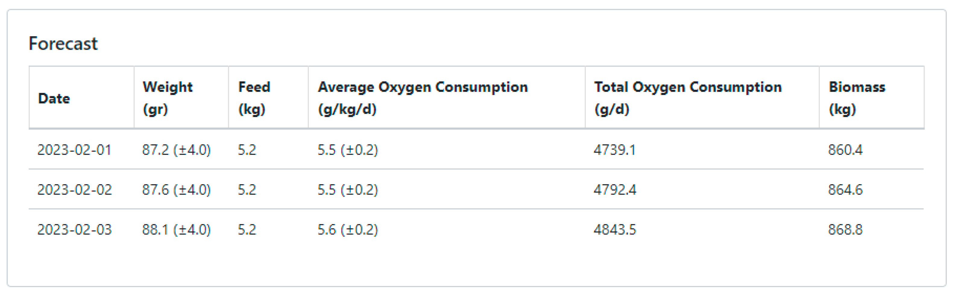
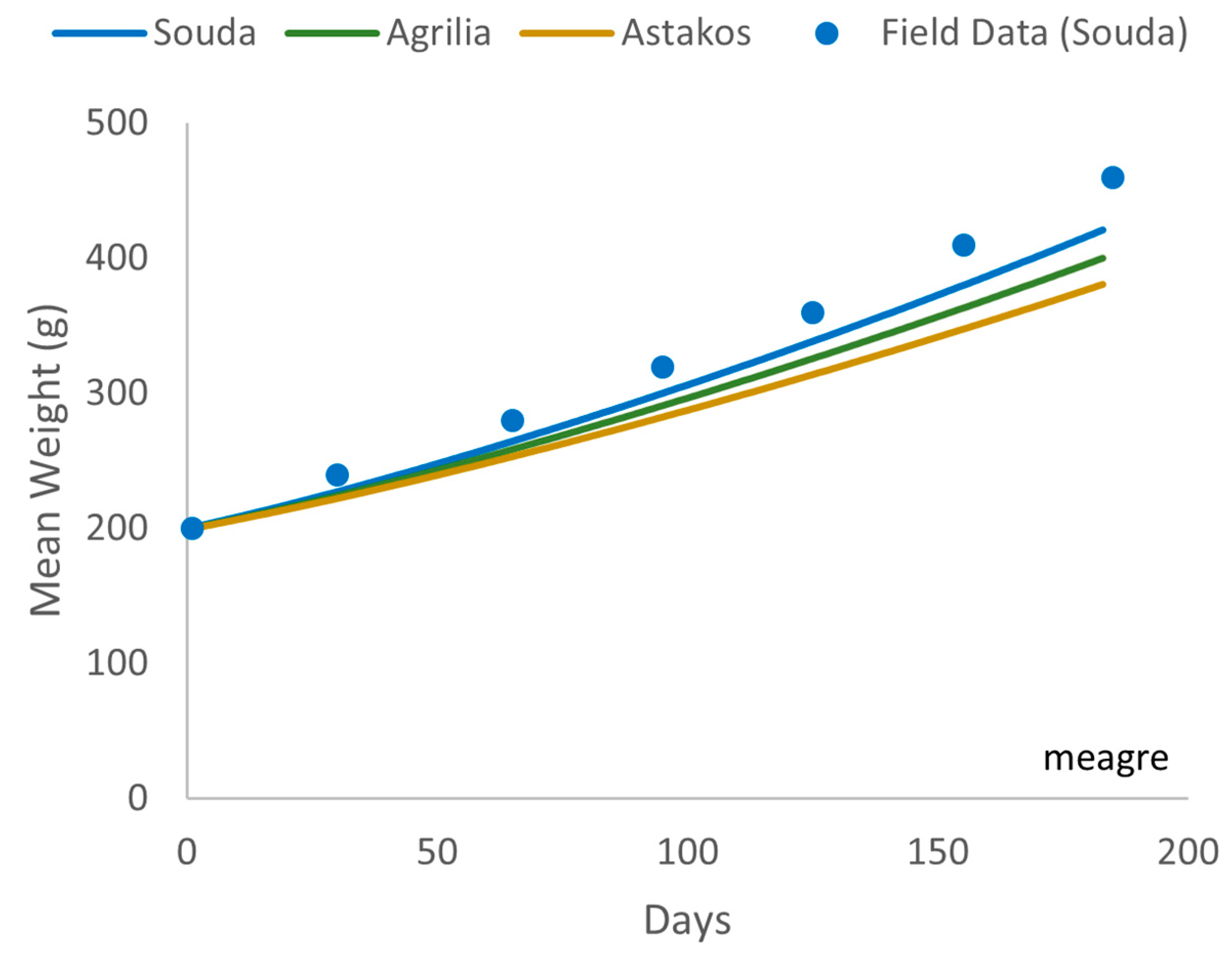