Comparison between Machine Learning and Deep Learning Approaches for the Detection of Toxic Comments on Social Networks

Abstract

The way we communicate has been revolutionised by the widespread use of social networks. Any kind of online message can reach anyone in the world almost instantly. The speed with which information spreads is undoubtedly the strength of social networks, but at the same time, any user of these platforms can see how toxic messages spread in parallel with likes, comments and ratings about any person or entity. In such cases, the victim feels even more helpless and defenceless as a result of the rapid spread. For this reason, we have implemented an automatic detector of toxic messages on social media. This allows us to stop toxicity in its tracks and protect victims. In particular, the aim of the survey is to demonstrate how traditional Machine Learning methods of Natural Language Processing (NLP) work on equal terms with Deep Learning methods represented by a Transformer architecture and characterised by a higher computational cost. In particular, the paper describes the results obtained by testing different supervised Machine Learning classifiers (Logistic Regression, Random Forest and Support Vector Machine) combined with two topic-modelling techniques of NLP, (Latent Semantic Analysis and Latent Dirichlet Allocation). A pre-trained Transformer named BERTweet was also tested. All models performed well in this task, so much so that values close to or above 90% were achieved in terms of the F1 score evaluation metric. The best result achieved by Transformer BERTweet, 91.40%, was therefore not impressive in this context, as the performance gains are too small compared to the computational overhead.

1. Introduction

The last few years have seen a true technological revolution. The global spread of the Internet and social networks has entered the daily lives of millions of people, forever changing the way they communicate. Sector experts define “cybercommunication” [1] as “communication via the Internet and social networks which, unlike traditional communication, takes place in a cultural context called cyberculture”, i.e., culture born from the application of new information and communication technologies in mass media such as the Internet. In this context, anonymity and the falsification of identities can give the user a feeling of absolute freedom, which can sometimes lead to inappropriate behaviour and even insults or harassment.

In recent years the dissemination of hate messages on social networks, so-called “hate speech”, has increased, along with the spread of offensive, abusive, insulting, degrading or obscene content directed at an individual or group of people, sometimes with tragic results. Therefore, according to [2], “a toxic comment is defined as a rude, disrespectful, or unreasonable comment that is likely to make other users leave a discussion”. Consequently, given the sheer volume of messages sent online every day, human moderation simply cannot guarantee complete control. For this reason, research into the detection of toxicity is essential, as the prompt removal of toxic messages to prevent them from spreading is the key to protecting victims. Hence, the European Court of Justice has ruled that from 2019, social platforms will be responsible for removing offensive content from their websites [3]. In addition, the EU court ruling, which explicitly mentions automatic detection systems, implicitly shows that these systems have a great social relevance.

The main contribution offered by this survey is an accurate comparison between three of the most commonly used Machine Learning (ML) classifiers in NLP challenges: Logistic Regression, Random Forest, and Support Vector Machine and the Transformer architecture, which represent the state of the art in Deep Learning (DL) text analysis, for the detection of toxic messages in social networks. In addition, ML models were also combined with two topic-modelling techniques: Latent Semantic Indexing (LSI) to perform dimensionality reduction and Latent Dirichlet Allocation (LDA) to focus on the topic discovery task, which automatically classifies each collected tweet according to its topic. A topic consists of a set of related terms. Contrary to what might be expected, the DL model contributes very little and has a higher computational cost than ML models. To determine this, classical evaluation metrics as well as computational cost and time are taken into account.

The manuscript is structured as follows. Section 2 cites some related work as the basis of our study. Then, Section 3 describes dataset and methods take into account in each experiment. Results are shown in Section 4 and their discussion is explained in Section 5. The last Section 6 deals with the conclusions.

2. Related Work

Given the need to develop an automated toxicity detection system as mentioned above, several authors have explored the application of Natural Language Processing (NLP) techniques to this purpose. Toxicity detection is a difficult problem, especially because toxicity comes in many forms, such as obscene language, insults, threats, hate speech and many other forms. Furthermore, the ambiguity of natural language and the flexibility of certain expressions, which may be offensive in one context but not in another, turn a simple detection approach into a fine-grained and delicate task. The idea, then, is to use sentiment analysis techniques and tools to study and analyse the information contained in a text in order to detect the emotions associated with an entity (person, group, context, etc.). An interesting paper on this approach is [4], where they explore the relationship between sentiment and toxicity in social network messages. Their results show that there is a clear correlation between sentiment and toxicity. In fact, using sentiment information improves the toxicity detection task, since it is possible for a user to mask toxic words by substitutions, but it is harder to mask the sentiment of a message.

Moreover, ref. [5] compared different sentiment classifiers, including Logistic Regression, Linear SVC and Naïve Bayes (NB), along with N-grams and Part-of-Speech (POS) tagging, to propose a method for detecting and classifying hate speech on Twitter. Their results show that NB achieved the best accuracy score, but they acknowledge that the accuracy of classifiers depends on the quantity and quality of the training dataset.

In addition, ref. [6] shows how metadata patterns could be used to create an algorithm for detecting online hate speech through the application of the Random Forest (RF) technique.

Other studies have been carried out such as [7], which compared different ML classifiers to identify the hate speech focused on two targets—women and immigrants—in English and Spanish tweets. The paper shows the comparison between different ML strategies in this particular task and concludes with SVM, Complement Naive Bayes and RF clearly outperforming the other classifiers and showing stable performance across all features.

The article [8] used Logistic Regression with L2 regularisation along with TF-IDF to accurately distinguish between everyday offensive language and serious hate speech, comparing a random sample of 25,000 English tweets from Hatebase.org. The paper warns of the potential for social biases in our algorithms.

In this context, it is interesting to examine another study [9], in which four sentiment analysis tools—VADER, TextBlob, Google Cloud Natural Language API and DistilBERT—were examined in order to highlight the difficulty of detecting toxicity to understand the presence of disability bias in sentiment analysis models. The results showed that posts related to people with disabilities (PWD) had significantly lower sentiment and toxicity scores as compared to posts not related to PWD. The results also showed how sentiment models built on social media datasets were most discriminatory against PWD.

Another approach to the problem was given by [10], where the effect of syntactic dependencies in sentences on the quality of the detection of toxic comments in social networks was studied. The article explains how the identification of toxic comments can be carried out in real time and with good quality by controlling three characteristics: the number of dependencies with proper nouns in the singular, the number of dependencies containing bad words, and the number of dependencies between personal pronouns and bad words.

3. Datasets and Methods

3.1. Dataset

The dataset used in this project consisted of nine different public datasets formed by tagged tweets, each dataset related to the detection of different typologies of toxicity in social networks (we chose nine files from the ones available at the following links to make up the whole starting dataset: https://github.com/AkshitaJha/NLP_CSS_2017, https://hasocfire.github.io/hasoc/2019/dataset.html, https://github.com/zeeraktalat/hatespeech, https://github.com/melsherief/hate_speech_icwsm18, https://ckan.hatespeechdata.com/dataset/founta-et-al-hate-and-abusive-speech-on-twitter/resource/9ccd6c1e-a7d2-4298-be72-fe78f529364e, https://www.kaggle.com/datasets/mrmorj/hate-speech-and-offensive-language-dataset, accessed on 20 June 2022); the main ones are:

• Hate Speech.
• Offensive Content.
• Sexism.
• Racism.

Therefore, when we merged the datasets to create a unique one, we preprocessed the entire set of tweets, taking care to adhere to the same labelling logic: “0”, neutral and “1”, toxic. Examples of neutral and toxic labelled tweets are, respectively:

• “True happiness is when we make our women smile. Celebrating the spirit of #WomensDay with the two most important women in my life”, “0”.
• “bro take it down u are just a fake ass friend and an ungrateful piece of shit u should be thank faggot”, “1”.

To have a better comprehension of the data, Figure 1 shows an overall datasets class proportion.

After the separate analysis, the nine sets were merged to obtain a single dataset consisting of 111,131 unique English-labelled tweets. We have 63,823 tweets belonging to class “0”, neutral, and 47,308 tweets belonging to class “1”, offensive, representing 57.43% and 42.57% of the total, respectively. The latter is the focus of the classification.

3.2. Preprocessing

Before the feature extraction, preprocessing is applied to the text in order to clean it and keep only those terms that provide real information for sentiment detection. It is possible to outline in points the action that the cleaning function will perform on our corpus:

• Removal of mentions and URLs from the text.
• Hashtags can provide value, so the # symbol is simply removed.
• Removal of punctuation marks.
• All text is made lowercase.
• Removal of words shorter than 2 characters.

It is important to note the role of emojis in qualifying the sentiment that the author of a message wants to convey, so it makes sense to develop two different cleanup functions, each resulting in a different set of data:

1.

Cleaned text and cleaned text and lemmatised text.

2.

Cleaned text and cleaned and lemmatised text, using the emoji (https://pypi.org/project/emoji, accessed on 3 July 2022) package to translate emotion icons into text strings and remove stop-words.

Both datasets were tested to compare the performance of each model. Finally, it should be noted that after each text cleaning function, duplicate tweets were detected and removed. This inevitably reduces the number of tweets but increases the quality of our data. In the end, we obtained 2 datasets depending on the cleaning function applied:

1.

100,105 tweets: cleaned and lemmatised text.

2.

98,701 tweets: cleaned, lemmatised, taking into account emojis and without stop-words.

For ease of reference, each dataset will be referred to by its respective number (1 or 2). It should be clearer if you look at the flowchart in Figure 2.

Once the text has been captured, cleaned up and the appropriate preprocessing transformations have been applied, it moves on to the feature extraction phase. When working with text, in order to make the text set usable for the learning task, it needs to be converted into numerical vectors. We have used two techniques to extract these vectors, so that they can be used by ML models:

• Bag of Words (BOW): A common vocabulary is created for all documents with all unique terms. A matrix of dimensions $n\times m$ is created, where n represents the number of documents and m the terms, and it is marked with 1 if the word is present in the text and with 0 if it is not [11,12].
• Term Frequency-Inverse Document Frequency (TF-IDF): Performs a weighting to promote the least common terms and discount the most frequent terms. This technique relates the number of times a term appears in a document (TF) to the number of documents in which it appears [13].

The major drawback of the two previous feature extraction techniques is the loss of the relationship between words and, as a consequence, the context of a document. To overcome this problem, we have used a third extraction technique:

• Word Embeddings: The idea is to assign to similar terms close vectors of a continuous and multidimensional vector space in a way that makes it possible to calculate similarities between words or sentences thanks to the distance between vectors, as well as to generalise a sentence into similar sentences, since the vectors will be similar [14].

3.3. Machine Learning

This section examines in detail the ML techniques used for Sentiment Analysis. In addition, it is important to emphasise that in these experiments we used sparse vectors resulting from the application of BOW and TF-IDF feature extraction.

The first model tested on the dataset was the Logistic Regression classifier to obtain a quick overview of the dataset. In fact, it is easy to implement and interpret, and very efficient to train, as well as having no hyperparameters to adjust. Another advantage of this model is that the Logistic Regression coefficients can be interpreted as indicators of the importance of the features. This aspect will also be discussed in Section 5 about model explainability.

The second step was to test the performance of the Random Forest (RF). It is an ensemble method (based on the divide-and-conquer intuition) of decision trees generated on a randomly divided data set, where each tree is voted on and the most popular class is chosen as the final result. It is simpler and more powerful than other non-linear classification algorithms.

The third test was to apply the Latent Semantic Analysis (LSA) technique [15] in combination with the Support Vector Machine (SVM) model. The idea is to use LSA to obtain a dimensional reduction of the dataset, as it is able to discover latent themes in a set of documents and to successively separate the two classes using an SVC model with a radial kernel.

Finally, we have applied the Latent Dirichlet Allocation (LDA) technique [16] and tested local models. The idea here is to divide our set of documents into subsets of related tweets and to treat each resulting subset separately in order to use each one with local models such as Logistic Regression and Random Forest.

3.4. Deep Learning

In order to exploit the semantic information of our messages, we used Word Embeddings as a feature extraction technique together with Transformers. In particular, we focused our efforts on the “BERTweet” model [17], available in the open source library “The Hugging Face” (https://huggingface.co/vinai/bertweet-base accessed on 12 August 2022, BERTweet is also available at https://github.com/VinAIResearch/BERTweet accessed on 12 August 2022). This model was chosen because it is a large-scale language model pre-trained with 850 million English tweets and has the same architecture as the BERT-base [18], is trained using the RoBERTa [19] pre-training procedure. So, it is suitable for our task.

All modelling was performed using the scikit-learn library [20] and the training procedure was carried out on the Google Colab Pro virtual machine.

4. Results

4.1. Logistic Regression

To perform these experiments, a random (70/30) dataset partition was chosen, but it is important to note that the test was repeated with 50 different seeds in order to obtain results as independent as possible in terms of the randomness factors of the dataset partition. Therefore, we calculated the standard deviation for each evaluation metric and visualised it on a graph to check how the standard deviation was bounded in the thousandths range.

Considering that the objective is to detect messages belonging to class 1, comparing the two F1-Score values obtained, BOW extraction combined with lemmatised text is the best option for both datasets:

Table 1. Logistic Regression results.

Dataset	Cleaning	FE	Accuracy	F1-Score	Precision	Recall
1	Lemma	BOW	0.9210	0.9073	0.9384	0.8783
2	Lemma	BOW	0.9206	0.9056	0.9379	0.8755

shows the Logistic Regression results.

4.2. Random Forest

From there, the datasets were divided into three sets: 70% training, 15% validation and 15% test. Once the best model configuration was chosen on the validation set, its generalisability was tested on the test set.

To find the best combination of hyperparameters, we made good use of the Cross Validation (CV) technique. The result was a model of 100 forest trees, each with a maximum depth of 80 and a minimum number of samples required to split an internal node of 10. We also used CV to configure the BOW feature extraction to further reduce the vocabulary size, ignoring terms with a document frequency strictly above the 0.2% threshold and strictly below the 0.0005% threshold.

Table 2. Random Forest results.

Dataset	Cleaning	FE	Accuracy	F1-Score	Precision	Recall
1	Lemma	BOW	0.9178	0.9007	0.9618	0.8469
2	Lemma	BOW	0.9188	0.9011	0.9578	0.8507

shows the results.

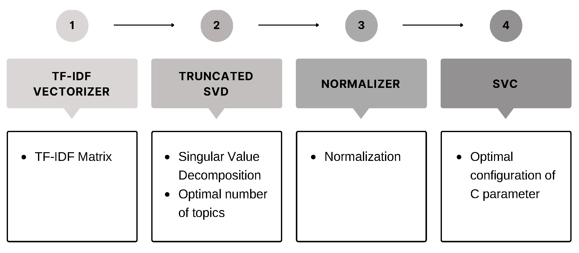
4.3. SVM with LSA

As mentioned in Section 3.3, we used the Latent Semantic Analysis (LSA) technique to apply a dimensional reduction to the dataset because of its ability to discover latent themes in a set of documents.

The steps performed to carry out this experiment can be summarised in the pipeline shown in Figure 3.

The application of LSA was very expensive in terms of computational time, so only dataset (1), with cleaned and lemmatised text, was tested, and the LSA tests were performed with three dimensions: 500, 1000 and 5000. The results shown in

Table 3. SVM with LSA results.

Dataset	Accuracy	F1-Score	Precision	Recall
1	0.9248	0.9112	0.9486	0.8767

refer to LSA with 5000 components and SVC with C = 4.

4.4. Transformer

A previous step worth mentioning is related to data cleaning, which is a bit different from the models seen so far because Transformers need a large amount of data to be able to find relationships between words [21]. For this reason, we tried to remove as little information as possible from our dataset, so we preferred to use the cleaned text of dataset (1) without removing stop-words and keeping emojis in their original format. The latter aspect was made possible by the fact that the BERTweet model adopts the RoBERTa pre-training procedure, as mentioned in Section 3.4. This type of procedure includes messages containing text and emojis so that its tokenizer recognises and supports these symbols.

With that brief introduction out of the way, let us move on to the description of the three tests that we wanted to run:

1.

Fine tuning of the Transformer’s Head layer, where all the weights are trained.

2.

Create a binary classification neural network (NN) just after the Transformer’s “Pooled Output” layer, training all the weights.

3.

Repeat point 2, freezing the Transformer’s weights and training only the output binary classification NN.

The results are summarised in

Table 4. BERTweet summary results.

Experiment	Dataset	Emojis	Accuracy	F1-Score	Precision	Recall
Fine Tuning	1	No	0.9238	0.9140	0.9084	0.9197
	1	Yes	0.9202	0.9108	0.8963	0.9259
NN	1	No	0.9241	0.9136	0.9158	0.9115
	1	Yes	0.9235	0.9133	0.9117	0.9150
NN freezing BERTweet	1	No	0.8326	0.7999	0.8444	0.7600

, where the best result in terms of F1-Score was achieved by training with four epochs, applying Head layers’ fine-tuning from the pre-trained model, with a 2 × 10${}^{-5}$ learning rate for the Adam optimization algorithm and a hidden dropout probability of 0.3.

4.5. LDA with Local Models

The LDA algorithm was used to extract three (value suggested by the topic coherence metric) main topics from the training data partition. Inferences were made on validation and test sets to assign each tweet to the corresponding topic. The next step was to save all the subsets separately to obtain three training sets, three validation sets and three test sets, each characterised by the same topic. All this allows us to divide the main dataset into three different partitions, each composed of tweets belonging to a topic detected by the unsupervised LDA algorithm. At this point, we proceeded to apply local models, such as Logistic Regression and Random Forest, on each partition. Once an evaluation metric had been calculated for each subset, we concatenated them to calculate the global metrics of the entire test set. Only in this way is it possible to compare the results with those obtained by the same model without applying LDA beforehand. The overall results obtained are summarised in

Table 5. LDA with local models global results.

Dataset	Cleaning	Model	Accuracy	F1-Score	Precision	Recall
1	Lemma	LR	0.9190	0.9046	0.9391	0.8726
1	Lemma	RF	0.8967	0.8788	0.9092	0.8504
2	Lemma	LR	0.9155	0.8987	0.9376	0.8628
2	Lemma	RF	0.9144	0.8973	0.9367	0.8611

.

5. Discussion and Future Work

Since the goal is to detect messages belonging to class “1”, comparing the F1-Score values shown in

Table 6. Summary results. * The AUC value is missing due to computational capacity issue, but it must be similar to the BERTweet’s one.

Model	Dataset	Cleaning	Accuracy	F1-Score	Precision	Recall	AUC
LR	1	Lemma	0.9210	0.9073	0.9384	0.8783	0.9165
RF	2	Lemma	0.9188	0.9011	0.9578	0.8507	0.9110
LSA+SVM	1	Lemma	0.9248	0.9112	0.9486	0.8767	/*
BERTweet	1	Cleaned	0.9238	0.9140	0.9084	0.9197	0.9248
LDA+LR	1	Lemma	0.9190	0.9046	0.9391	0.8726	0.9140
LDA+RF	2	Lemma	0.9144	0.8973	0.9367	0.8611	0.9085

, we see that the ML models perform slightly worse than the Transformer model, but essentially at the same level. We can also look at the AUC column, which indicates how well the model is able to discriminate between classes. The higher the AUC, the better the model is at predicting ‘0’ classes as ‘0’ and ‘1’ classes as ‘1’. Similarly, the higher the AUC, the better the model is at discriminating between toxic and non-toxic messages. This can also be seen in the comparison graph in Figure 4, where it is clear that all models have a similar ROC curve.

LSA with SVM is the ML combination that comes closest to BERTweet. This suggests to us a possible future work: it is worth testing LSA with a higher number of components (e.g., 10,000) and an SVC model with a C-parameter greater than 4 in order to optimise its global performance.

At the same time, the slight difference in terms of performance between the simpler Logistic Regression model and the more complex Transformer model could be compensated by the model explainability. For this purpose, it might be helpful to look at

Table 7. Logistic regression coefficients for the 10 most significant words of each class.

Class 0		Class 1
Word	Coeff	Word	Coeff
andre	3.2909	bitch	6.9165
repost	2.4319	bitches	6.8372
digging	2.0458	faggot	6.6135
alabama	1.8461	retard	6.4470
delivery	1.8286	pussy	6.2022
adaywithoutwomen	1.7918	twat	6.0638
womensday	1.7909	nigger	5.8509
latest	1.7093	hoes	5.7620
movie	1.6863	retarded	5.5095
amazon	1.6858	niggah	5.1660

, which shows the most significant words and their corresponding LR coefficients.

The fact that BERTweet achieved a slightly better result is probably due to its ability to understand context, unlike other ML models. However, it is also true that our dataset collected individual tweets rather than whole dialogues, so this fact could minimise the potential of the Transformer and cause the model to focus mainly on significant words, reducing the performance gap between ML models. For this reason, another interesting future work is to re-train BERTweet on the same dataset but with these words masked, forcing it to try to find relationships and contexts of toxicity beyond the terms used.

Another interesting aspect is the versatility and ambiguity of natural language, which offers many ways of writing offensive comments without necessarily using swearwords, but, for example, by referring to an external fact or assumption that an algorithm cannot directly extrapolate from the text but that a human can.

At the same time, being able to rely on a dataset that includes entire conversations allows us to extrapolate contextual information about the sentiment of each message, monitor the conversation and detect unruly toxic comments that correspond to sudden changes in conversation sentiment.

Furthermore, it would be interesting to analyse the misclassification messages distinguishing between false positives (non-toxic comments that are misclassified as toxic) and false negatives (toxic comments that are misclassified as non-toxic) to improve the model’s explainability and give us the opportunity to solve the toxicity detection problem more efficiently.

6. Conclusions

The aim of this research was a comparative analysis of the most used Machine Learning classification models against the state of the art in Deep Learning, represented by BERTweet, focusing on the automatic detection of toxic messages in social networks.

Using NLP techniques related to sentiment analysis, different models such as Logistic Regression, Random Forest, Support Vector Machine and Transformer were trained on the same dataset.

Comparing the results of the experiment shown in Table 6, the BERTweet model can automatically detect toxic tweets with a rate of 91.40% in terms of F1-Score, but at a high computational cost. In fact, Transformer requires powerful hardware to cope with the complexity of its architecture, such as the number of trainable parameters, and this fact is also reflected in terms of training and inference time as shown in

Table 8. Computational time. To facilitate time comparison among different models, we divide the total time of training and inference tasks by the number of tweets of each dataset, so results shown in Training Time [µs] and Inference Time [µs] columns represent the average time of single tweet in microseconds. Regarding Transformer, the average training time is referred to as 1 epoch. * Time information about LSA combined with the SVM model could not be computed under the same conditions, since the virtual machine used for time measurements did not have enough computational capacity to run this model.

Model	Dataset	Cleaning	Training Time	Inference Time
LR	1	Lemma	38	14
RF	2	Lemma	187	43
LSA+SVM	1	Lemma	/*	/*
BERTweet	1	Cleaned	11,192	5754
LDA+LR	1	Lemma	2247	573
LDA+RF	2	Lemma	3163	784

.

As a matter of fact, if we focus on the results obtained by the other methods, we can see that they all performed well, reaching values around or above 90% in terms of F1-Score and proving to be much faster both in terms of training time and inference time compared to BERTweet’s performance.

Furthermore, Figure 4 highlights how all models have the same ROC curve, so the performance of the classification model is almost the same at all classification thresholds. This shows that the Transformer does not offer much improvement in solving this task, as the performance gains are too small compared to the computational overhead.

References

- Arab, L.E.; Díaz, G.A. Impact of social networks and internet in adolescence: Strengths and weaknesses. Rev. Medica Clin. Condes 2015, 26, 7–13. [Google Scholar]
- Risch, J.; Krestel, R. Toxic Comment Detection in Online Discussions. In Deep Learning-Based Approaches for Sentiment Analysis; Springer: Singapore, 2020; pp. 85–109. [Google Scholar]
- Modha, S.; Mandl, T.; Majumder, P.; Patel, D. Overview of the HASOC track at FIRE 2019: Hate Speech and Offensive Content Identification in Indo-European Languages. In Proceedings of the 11th Forum for Information Retrieval Evaluation—FIRE ’19, Kolkata, India, 12–15 December 2019; Volume 2517, pp. 14–17. [Google Scholar]
- Brassard-Gourdeau, E.; Khoury, R. Subversive Toxicity Detection using Sentiment Information. In Proceedings of the Third Workshop on Abusive Language Online, Florence, Italy, 1–2 August 2019; pp. 1–10. [Google Scholar]
- Kiilu, K.K.; Okeyo, G.; Rimiru, R.; Ogada, K. Using Naïve Bayes Algorithm in detection of Hate Tweets. Int. J. Sci. Res. Publ. 2018, 8, 99–107. [Google Scholar] [CrossRef]
- Miró-Llinares, F.; Moneva, A.; Esteve, M. Hate is in the air! However, where? Introducing an algorithm to detect hate speech in digital microenvironments. Crime Sci. 2018, 7, 15. [Google Scholar] [CrossRef]
- Almatarneh, S.; Gamallo, P.; Pena, F.J.R.; Alexeev, A. Supervised Classifiers to Identify Hate Speech on English and Spanish Tweets. Digit. Libr. Crossroads Digit. Inf. Future 2019, 11853, 25–30. [Google Scholar]
- Davidson, T.; Warmsley, D.; Macy, M.; Weber, I. Automated Hate Speech Detection and the Problem of Offensive Language. arXiv 2017, arXiv:1703.04009. [Google Scholar] [CrossRef]
- Venkit, P.N.; Wilson, S.K. Identification of Bias Against People with Disabilities in Sentiment Analysis and Toxicity Detection Models. arXiv 2021, arXiv:2111.13259. [Google Scholar]
- Shtovba, S.; Shtovba, O.; Petrychko, M. Detection of Social Network Toxic Comments with Usage of Syntactic Dependencies in the Sentences. In Proceedings of the Second International Workshop on Computer Modeling and Intelligent Systems, CEUR Workshop 2353, Zaporizhzhia, Ukraine, 15–19 April 2019. [Google Scholar]
- Qader, W.A.; Ameen, M.M.; Ahmed, B.I. An Overview of Bag of Words;Importance, Implementation, Applications, and Challenges. In Proceedings of the 2019 International Engineering Conference (IEC), Erbil, Iraq, 23–25 June 2019; pp. 200–204. [Google Scholar]
- Li, Y.; Li, T.; Liu, H. Recent advances in feature selection and its applications. Knowl. Inf. Syst. 2017, 53, 551–577. [Google Scholar] [CrossRef]
- Robertson, S. Understanding Inverse Document Frequency: On Theoretical Arguments for IDF. J. Doc. 2004, 60, 503–520. [Google Scholar] [CrossRef]
- Mikolov, T.; Chen, K.; Corrado, G.; Dean, J. Efficient Estimation of Word Representations in Vector Space. arXiv 2018, arXiv:1301.3781. [Google Scholar]
- Wiemer-Hastings, P. Latent Semantic Analysis. Encycl. Lang. Linguist. 2004, 2, 1–14. [Google Scholar]
- Blei, D.M.; Ng, A.Y.; Jordan, M.I. Latent Dirichlet Allocation. J. Mach. Learn. Res. 2003, 3, 993–1022. [Google Scholar]
- Nguyen, D.Q.; Vu, T.; Nguyen, A.T. BERTweet: A pre-trained language model for English Tweets. In Proceedings of the 2020 Conference on Empirical Methods in Natural Language Processing: System Demonstrations, Online, 16–20 November 2020; Association for Computational Linguistics: Cedarville, OH, USA, 2020; pp. 9–14. [Google Scholar]
- Devlin, J.; Chang, M.-W.; Lee, K.; Toutanova, K. BERT: Pre-training of Deep Bidirectional Transformers for Language Understanding. arXiv 2018, arXiv:1810.04805. [Google Scholar]
- Liu, Y.; Ott, M.; Goyal, N.; Du, J.; Joshi, M.; Chen, D.; Levi, O.; Lewis, M.; Zettlemoyer, L.; Stoyanov, V. RoBERTa: A Robustly Optimized BERT Pretraining Approach. arXiv 2019, arXiv:1907.11692. [Google Scholar]
- Pedregosa, F.; Varoquaux, G.; Gramfort, A.; Michel, V.; Thirion, B.; Grisel, O.; Blondel, M.; Müller, A.; Nothman, J.; Louppe, G.; et al. Scikit-learn: Machine Learning in Python. arXiv 2012, arXiv:1201.0490. [Google Scholar]
- Vaswani, A.; Shazeer, N.; Parmar, N.; Uszkoreit, J.; Jones, L.; Gomez, A.N.; Kaiser, L.; Polosukhin, I. Attention Is All You Need. arXiv 2017, arXiv:1706.03762. [Google Scholar]