Abstract
Forecasting flight fares is a critical task in the rapidly expanding civil aviation industry and involves numerous factors. However, traditional airfare prediction systems are ineffective due to the complex and nonlinear relationships of multiple factors, which are not able to accurately account for the impact of different attributes such as time period. To tackle these issues, in this study, we proposed a novel approach that utilizes a deep-learning model, specifically, the Gated Recurrent Unit (GRU), by incorporating 44 decision features. The proposed model is able to capture the intricate relationships between various factors effectively and predict air ticket prices with high accuracy. In the experiments, it was found that the GRU model significantly outperforms not only classic machine learning models but also the MLP and LSTM in terms of assessment indicators of mean absolute error (MAE), root mean square error (RMSE), and coefficient of determination (R2). The GRU model is thus promising concerning the fare prediction of flight tickets.
1. Introduction
Finance is critical in our daily economic activities, and accurate financial forecasts may help economic growth [1,2,3,4]. However, the modern global market is complicated, chaotic, and dynamic and may be influenced by diverse factors; thus, price prediction becomes a challenging task [4,5]. Recently, some studies have been conducted to address this issue, with a focus on machine learning techniques [6,7]. Approaches to price prediction are inclined toward machine learning (ML) as machine learning algorithms can not only learn to identify patterns or correlations within training data but also achieve excellent predictive capability for unseen data. Machine learning techniques have been used to predict customer behavior [8], market trends, and subsequent prices based on historical data [9,10,11]. On the other hand, decision-making and decision support in business are other essential issues in finance but are not easy to address since non-optimal short-term decisions are sometimes preferred or required in order to achieve long-term strategic goals [3,12]. ML models have also been proposed to optimize business policies to make sequential decisions toward a long-term objective [13].
Due to the excellent performance and nobility of deep learning [9,14,15], it has recently attracted much attention in computer vision, natural language processing, and finical prediction [15,16]. Deep learning research has undergone rapid development in recent years and has been successfully applied to a wide variety of areas [17]. It has achieved good performance in quantitative investment, risk control, and other areas [18]. For price prediction, various deep learning algorithms have been used, and RNN is one of them [19]. RNN is well-suited to time series forecasting since it can process variable-length sequences of incoming data in its internal memory. RNN-based models have been successfully applied to the predictions of future prices [20], and long short-term memory (LSTM) and gated recurrent unit (GRU) are the top options [18,21]. They can also be used together with conventional ML-based prediction models, such as decision trees, genetic algorithms [22], and support vector machines [23], for the prediction of prices. Notice that the trend exhibited by the flight ticket fare is highly complex and nonlinear [24]. Conventional forecasting methods based on a linear model, such as linear regression, therefore faces a number of challenges. A deep neural network that is able to better model highly nonlinear changes is hence promising for such purposes.
Additionally, financial prediction is complicated due to the fact that there are many features of the series that have varying degrees of influence or importance [13]. Among these features, however, only a few have higher impacts on the trend of the series and convey the most relevant information overall. It is, therefore, necessary for prediction or analysis methods to identify salient and influential features from a large amount of data. For RNN, the gated recurrent unit was shown to be able to prioritize relevant features, allowing for more efficient extraction in short-term mode and preventing data loss due to lengthy time series [25]. Therefore, in this research, we propose the use of the GRU model for RNN, considering its ability to learn to capture correlations between flight ticket fares and relevant features.
On the other hand, a lack of appropriate data is a major impediment to the advancement of studies on projecting future fares of flight tickets [22]. Since ticket prices are extremely sensitive to business interests, they are seldom disclosed, and the vast majority of airlines do not make their pricing plans known to the public. Despite the limited resources available, a few publications have developed a range of methodologies for predicting ticket prices [26,27]. In this research, we used historical flight data from Ethiopian Airlines, which is the oldest and leading airline in Africa, for the purpose of this study. The data ranged from January 2018 to July 2022, and there were more than 1,000,000 records from 22 domestic and international airline destinations. The sufficiency and quality of the data make the analysis results credible.
The key contributions of this study are summarized as follows:
- The results obtained from the GRU model demonstrate a significant impact and provide valuable insights for ongoing research in this area.
- The research introduces a novel approach employing a deep-learning GRU model for fare prediction. This method addresses the limitations of traditional machine learning techniques that rely heavily on statistical variables in their models.
- The GRU model leverages its unique architecture to capture temporal dependencies in flight data, resulting in improved predictive performance.
2. Related Work
With advancements in machine learning, price forecasting techniques have made significant strides in diverse industries [28], such as agriculture, stock, bitcoin, and oil [29,30,31]. Recent studies on flight fare prediction have utilized mainly machine learning approaches. A study discussing the challenge of air ticket fare prediction shows that its variability and dependence on various factors lead to revenue losses and customer dissatisfaction [32]. This research proposed an ensemble model using neural networks, XGBoost regressor, and light gradient boosting machine regression to estimate flight ticket fares with the least mean absolute error. The dataset contained flight ticket data from March to June 2019 for various airlines. Airlines can plan their strategies of operations and allocate necessary resources according to predicted ticket prices so as to impact specific market segments. Another study compares the prediction performances of flight ticket prices based on eight regression models, including multilayer perceptrons, generalized regression neural networks, extreme learning machines, random forest regression trees, and so on [33]. This study aimed to identify the factors that impact airfare, such as departure and arrival times, the amount of free luggage allowed, the days before departure, and so on. The models were trained on a dataset containing 1814 flights for a single international route, and the results indicated that the model “bagging regression tree” achieved the highest accuracy, followed by the random forest model. Additionally, in another study, random forest and multilayer perceptron models were trained individually and combined with assigned weights to form a stacked prediction model [34], which was shown to outperform the individual models. The data used to train the models consisted of 51,000 records for a 7-day round trip nonstop flight with three domestic airlines. Twelve features were extracted from the data, including the airline, flight number, date of purchase, departure date and time, and so on. The stacked prediction model outperformed the random forest and multilayer perceptron models with 4.4% and 7.7% improvement, respectively, based on the R2 metric.
Furthermore, a new model was proposed to predict the minimum available price for a particular itinerary, i.e., a specific flight on a given route for a specific departure date [26]. To achieve this, a modified ensemble-based learning algorithm was proposed to learn from past patterns of price changes and make forecasts for future prices. This study utilized a recursive approach to predict future prices sequentially. The model used various features, including prices of the same itinerary, recent itineraries, and itineraries for the same day of the week or month. The experimental results demonstrated that the model performed best on diverse routes, where different flights have independent pricing behaviors. A comparison of the algorithms showed that the proposed model based on ensemble learning was superior to KNN. Table 1 shows the summary of related works.

Table 1.
Summary of related works on the prediction of flight ticket fares.
3. Methodology
3.1. Data Source
A combination of high-quality data sources and effective feature engineering can significantly improve the results of machine learning research and help to achieve accurate and meaningful predictions [23]. In this research, the data were sourced from Ethiopian Airlines. Despite its humble beginnings, Ethiopian Airlines has had a successful 75-year journey that has positioned it as Africa’s leading aviation group [8,36]. The data used in this study covered a period from January 2018 to July 2022 and comprised a total of 1,032,215 records from 22 domestic and international destinations served by the airline. This extensive dataset provided a robust foundation for machine learning research and could yield valuable business insights. Table 2 displays a few samples that contain a part of the data, including the origin, destination, and type of flight.
Table 2.
A few samples of the flight data.
3.2. Preliminary Data Analysis
Data visualization is essential for interpreting complex datasets, allowing users to make sense of a large amount of information quickly and efficiently [37,38]. The data ranged from January 2018 to July 2022, and there were more than 1,000,000 records from 22 domestic and international airline destinations. As we dove into analyzing this vast dataset, it became crucial to present the findings in an easily interpretable way so as to bring about the insights intuitively. We employed data visualization techniques to reveal patterns, trends, and correlations that would otherwise have been challenging to discern. Figure 1 shows the relationship between travel dates and flight ticket fares (in USD), with six subfigures depicting different aspects of the data. Figure 1a–e display the monthly averages of flight ticket fares for the year 2018 through the year 2022 (up to July), which reveal information regarding price changes over time. Figure 1f further presents a more granular view of the data that depicts the daily fares of flight tickets for the entire dataset. Collectively, these subfigures give an overview of trends and fluctuations concerning prices for the whole dataset.
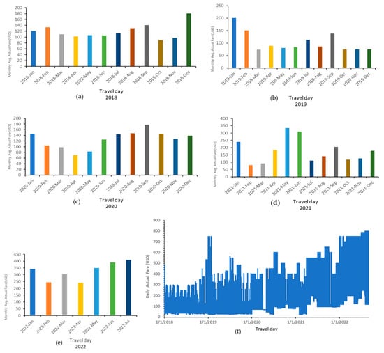
Figure 1.
Flight ticket fares versus time periods. (a–e) monthly averages for year 2018 through year 2022 (up to July) and (f) daily fares of flight tickets for the whole dataset.
Additionally, Figure 2 presents a boxenplot of flight fares versus booking classes. The boxenplot is a commonly used statistical tool that displays the distribution of a dataset and highlights such key features as the median, quartiles, and outliers. Unlike a traditional boxplot, the boxenplot divides the data into smaller subgroups, allowing for a more detailed view of the distribution. In this case, we used the boxenplot to examine the relationship between the flight fare and the booking class, which is the letter code used by the airline to identify the fare type and restrictions of a ticket. By analyzing the boxenplot, we were able to identify the ranges of ticket fares as well as the potential outliers or anomalies that might have an impact on our analysis. This initial exploration served as a foundation for our subsequent pilot analysis, allowing us to better understand the data beforehand. Furthermore, the correlations between the features were computed, and a few of them are selected and displayed in Table 3. As can be observed from Table 3, some features, such as Holiday, Week Day, Seg_Dest, and Class of Service, are highly correlated to the Actual Fare. The preliminary data analysis, consisting of descriptive statistics and correlation techniques, has provided valuable insights into the key factors that impact flight ticket prices. These insights were instrumental in the development of an accurate prediction model.
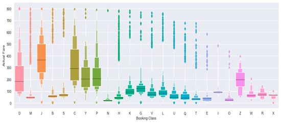
Figure 2.
Boxenplot of flight ticket fares versus booking classes.
Table 3.
A sample of the correlations between features.
3.3. Data Preprocessing
To improve the quality of the data, data preprocessing techniques were applied to the raw data collected from the sources. Figure 3 shows the overall data processing stages. Some errors in the raw data were first corrected in the data cleaning stage, and feature engineering was then conducted. Feature engineering involves creating new features from existing data fields to enable the model to better capture underlying patterns within data. Based on the data analysis in the previous section, a few new features, including Season, Travel Day, Travel Month, IsWeekend (Yes/No), IsHoliday (Yes/No), and NumOfStops, etc., were created, as listed in Table 4. These features exhibit specific characteristics of the flight data that influence ticket fares and are meaningful for business decisions. For instance, Season and Travel Month might indicate long-term seasonal demand for flights, while IsWeekend could help to identify the price difference between weekends and weekdays. Similarly, IsHoliday can be used to analyze whether or not prices change during holidays. The feature NumOfStops may be helpful for differentiating prices between direct and connecting flights. Overall, those features provide a comprehensive view of flight data and help build a more reliable prediction model since they are correlated to flight ticket fares.
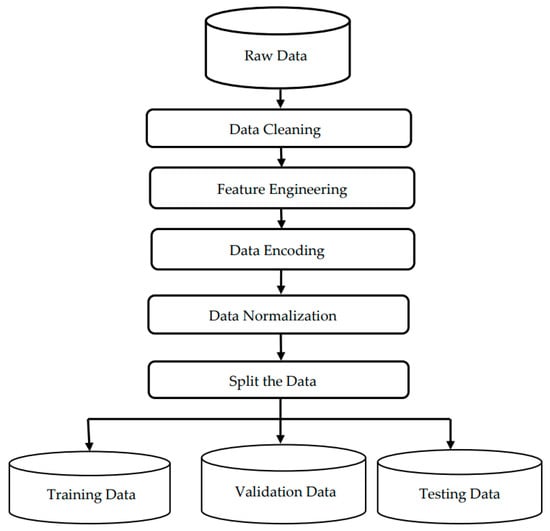
Figure 3.
Data preprocessing stages.
Table 4.
A few selected features used in the fare prediction model.
To prepare the data for the machine learning algorithms, we further applied two data transformation techniques: data encoding and data normalization. In data encoding, the categorical features were converted into numerical representations by one-hot encoding in the form of binary vectors such that the features were acceptable for most ML algorithms. Next, numerical data such as ticket fare were normalized into the region between 0 and 1 according to their dynamic range based on the following formula:
where and denote the maximum and minimum values of the feature, respectively. Data normalization ensures that the numerical features of various flights are on compatible scales so as to have similar impacts on the prediction model. Finally, the preprocessed data were split into training, validation, and testing datasets with 44 decision features. The training dataset was used to train the model, the validation dataset was used to evaluate the performance during training, and the unseen testing dataset was used to assess the generalization capability of the model.
3.4. Long Short-Term Memory
Recurrent Neural Networks (RNNs) have gained popularity in the field of machine learning for their ability to model sequential data. In RNNs, information is propagated through a chain of connected nodes, with the input sequence data processed in the direction of sequence evolution [39,40]. RNNs have the inherent capacity to memorize and incorporate past information, which has led to their successful application in time series prediction. However, despite the potential of RNNs, their performances can be affected by certain factors. When the length of the input sequence increases, for example, the network layers greatly expand, which usually leads to the problem of gradient vanishing [41].
Long short-term memory (LSTM) is a type of recurrent neural network with a deep architecture [42,43]. Its unique gate mechanism and structure significantly enhance the model’s memory capacity and alleviate the problem of gradient disappearance that is often encountered when training classical RNNs on very long input sequences [44]. Figure 4 depicts the network layout of one neural unit of LSTM. The LSTM neural network is composed of several gates and variables. The input gate, , regulates how much new information is added to the cell state at each time step. The forgetting gate,, determines how much information from the previous cell state should be retained. The output gate, , regulates how much information should be output from the current cell state. The input channel state, , is obtained by compressing the messages from the input state, , and the previous hidden state, , with the tanh function, and might be added to the cell state, under the control of the input gate . The cell state denotes the long-term memory in general that could be forgotten through the forgetting gate, .
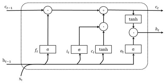
Figure 4.
Internal structure of an LSTM unit.
The process by which every LSTM unit updates its parameters is as follows:
where is the sigmoid function that makes a gate act as a switch. , , and are the weight matrixes of the forget gate, input gate, and output gate, respectively. , , , and are the biases of the forget gate, input gate, output gate, and input channel, respectively.
3.5. GRU Model
The gated recurrent unit (GRU) is another type of recurrent neural network that can handle sequential regression problems [45,46]. GRU is able to memorize and retain important information from past observations in the sequence and is conceptually similar to LSTM [19,47]. GRU is faster to train and less prone to overfitting, especially when working with large datasets or limited computational resources. This advantage is particularly relevant for airfare prediction, which often involves handling massive datasets with complex patterns. Another advantage of GRU is its efficiency in capturing long-term dependencies and relationships within time series data [48]. In airfare prediction, this is crucial for capturing factors such as seasonal trends, holidays, and economic fluctuations, which can significantly impact prices over time. GRUs have been shown to effectively capture such relationships, resulting in accurate airfare predictions. In addition, GRUs are less sensitive to the gradient vanishing problem, which can occur in traditional RNNs when learning long-term dependencies [49]. This makes GRUs more robust and better suited for tasks involving lengthy sequences, such as airfare prediction. Moreover, GRUs can be combined easily with other neural network architectures or feature engineering techniques to improve prediction accuracy. All these make GRUs highly adaptable and suitable for tackling complex prediction tasks [3,31].
Figure 5 displays the internal network structure of a GRU unit. In Figure 5, represents the reset gate, represents the update gate, and denotes the input state, while and represent the previous and current hidden states, respectively. The symbols W, U, and b are the learnable weights and biases of the network.
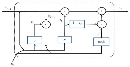
Figure 5.
Internal structure of a GRU unit.
The states of a GRU unit are updated according to the formula below:
Equation (8) computes the update gate , which determines how much of the previous hidden state should be preserved, and how much should be replaced by the new information in . The sigmoid function, , squeezes the input into the range [0, 1]; thus, is a value between 0 and 1. Equation (9) computes the reset gate , which determines how much of the previous hidden state should be forgotten, and how much should be used to compute . Like , is also a value between 0 and 1. Equation (10) computes the candidate hidden state , which is a new value that is mixed with the previous hidden state based on the update gate . The hyperbolic tangent function, tanh, compresses the input into the range [−1, 1]. Finally, Equation (11) computes the new hidden state as a linear combination of the previous hidden state, , and the candidate hidden state, , weighted by the update gate, . The symbol represents element-wise multiplication, and 1 − represents the complement of . This ensures that the new hidden state combines only the relevant information from and . The architecture of the GRU unit, with its gating mechanisms, allows for better control over the flow of information through the network and has been shown to be excellent in a diverse range of tasks. The GRU network structure is presented in Figure 6. The implementation of the GRU model is shown in Algorithm 1, which is based on the Pytorch framework.
| Algorithm 1. Stacked GRU flight fare prediction model. |
| #Step 1: Define the StackedGRU class class StackedGRU(nn.Module): #Step 2: Define the constructor to initialize the model parameters def __init__(self, input_size, hidden_size, output_size, num_layers, dropout, window_size=1): super(StackedGRU, self).__init__() #Step 3: Set the model parameters self.input_size = input_size # Size of input layer self.hidden_size = hidden_size # Size of hidden layers self.output_size = output_size # Size of output layer self.num_layers = num_layers # Number of layers in the stacked GRU model self.dropout = dropout # Dropout probability self.window_size = window_size # Number of time steps to include in each window #Step 4: Create a list of GRU layers self.gru_layers = nn.ModuleList() #Step 5: Add the first GRU layer self.gru_layers.append(nn.GRU(input_size, hidden_size, batch_first=True, dropout=dropout)) #Step 6: Add additional GRU layers if num_layers > 1 for i in range(num_layers-1): self.gru_layers.append(nn.GRU(hidden_size, hidden_size, batch_first=True, dropout=dropout)) #Step 7: Create the output layer self.linear = nn.Linear(hidden_size * window_size, output_size) #Step 8: Define the forward pass through the stacked GRU model def forward (self, x): #Step 9: Reshape the input into windows of size self.window_size x = x.view(x.shape[0], -1, self.window_size, self.input_size) #Step 10: Transpose the input to (batch_size, window_size, sequence_length, input_size) x = x.transpose(1, 2) #Step 11: Flatten the input to (batch_size * window_size, sequence_length, input_size) x = x.contiguous().view(-1, x.shape[3], x.shape[2]) #Step 12: Pass the input through each GRU layer in the stacked model for i in range(self.num_layers): #Step 12a: Get the current GRU layer output, _ = self.gru_layers[i](x) #Step 12b: Apply dropout to the output output = F.dropout(output, p=self.dropout, training=self.training) #Step 12c: Set the input for the next layer to be the output of the current layer x = output #Step 13: Reshape the output to (batch_size, window_size, hidden_size * sequence_length) output = output.contiguous().view(-1, self.window_size, output.shape[2] * output.shape[1]) #Step 14: Flatten the output to (batch_size * window_size, hidden_size * sequence_length) output = output.view(-1, output.shape[2]) #Step 15: Pass the final output through the output layer out = self.linear(output) #Step 16: Reshape the output to (batch_size, window_size, output_size) out = out.view(-1, self.window_size, self.output_size) |
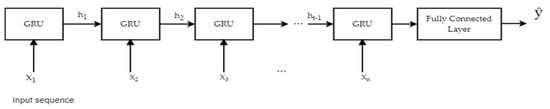
Figure 6.
Network structure of GRU model.
A GRU model is a powerful algorithm for predicting time series data, particularly when dealing with nonlinear features [25]. However, building an effective GRU model for prediction tasks is not straightforward. Models with too few layers may struggle to capture the nonlinearity of fluctuating features, while models with too many layers may take too long to train and are prone to overfitting. In this study, we investigated its effectiveness in predicting flight ticket fares, which are influenced by a variety of factors. By leveraging the peculiarities of airline ticket fare series, the predictive abilities of the GRU model can be enhanced. After conducting a number of experiments, we developed a stacked GRU model that balances performance and efficiency.
Our experimental architecture is shown in Figure 7, which involved two main stages: offline learning and online prediction. During offline learning, the model is trained on the training data and evaluated with the validation data. Once the model is trained, it is used in the prediction process to efficiently predict flight ticket fares. In addition, the prediction performance of the flight ticket fares for the model is finally evaluated with the unseen testing data based on mean absolute error (MAE), root mean square error (RMSE), and coefficient of determination (R2). The hyperparameters chosen for the model are listed in Table 5, which will be used in later experiments.
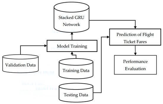
Figure 7.
Experimental architecture for flight fare prediction.
Table 5.
Hyperparameter setting for the prediction model.
4. Experiments and Discussion
The performance of the proposed GRU model was compared with that of the MLP and LSTM. During the training process, a number of parameters, such as batch size, activation function, number of hidden units, type of optimizer, and number of epochs, were adjusted until the best possible model was obtained. Four optimizers, including Adam, Adamax, RmsProp, and Sgd, were tested to minimize the loss. The losses with respect to the number of epochs for the four optimizers are compared in Figure 8. It can be observed from Figure 8 that the Adam optimizer converged much faster than the other three. Therefore, the Adam optimizer was adopted to train the models in the following experiments.
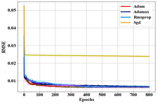
Figure 8.
Convergence of loss for different optimizers.
Furthermore, the prediction performance was evaluated with three metrics, described as follows. Mean absolute error is the average of the absolute difference between the target value and the predicted output.
Here, denotes the actual value of the flight ticket fare, denotes the predicted value, and N denotes the number of samples. MAE is a commonly used metric since it provides an intuitive indicator of the extent to which the predicted values deviate from the actual values on average. MAE is easy to interpret, suitable for continuous variables, and less sensitive to outliers, which means it is robust and can give a good overview of a model’s performance [50].
Root mean square error (RMSE) is another metric widely used to evaluate prediction models. It is the objective function used for optimizing classic regression models. RMSE is computed as follows:
where represents the actual value of the flight ticket fare, represents the predicted value of the flight ticket fare, and N denotes the number of samples. RMSE is the standard deviation of predictions from a stochastic point of view. A small value of RMSE is indicative of a model with excellent performance.
Additionally, the coefficient of determination, usually denoted as , is a metric for evaluating how well a regression model performs in a number of analyses [51]. The computation of is formulated as follows:
where is the mean of the total amount of data, is the actual value of the flight ticket fare, and is the predicted flight ticket fare. is the sum of squared prediction errors for the proposed model, TSS is the squared sum of the errors between the actual value and the mean of all outputs, and N is the number of samples. TSS denotes the error of the simple predictor, which simply takes the mean of all observations as the predicted output. A small ratio of RSS to TSS, corresponding to a high R2, means that the error of the prediction model is much smaller than that of that simple predictor, and the model is hence considered to be effective. The value of R2 usually falls between 0 and 1; when R2 is close to 1, this indicates that the model fits the data well in a number of analyses. A high value of R2 means that the model could explain a large portion of the variance in the target variable, while a low value of R2 suggests that the model cannot capture much of the variation in the data. In summary, R2 is a useful metric for comparing regression models so as to determine the overall fit of a model.
Figure 9 depicts a comparison of the convergence speed of the GRU, LSTM, and MLP models. As can be observed from Figure 9, the GRU model outperformed the others in RMSE. The loss of the GRU model was significantly lower than that of the others.
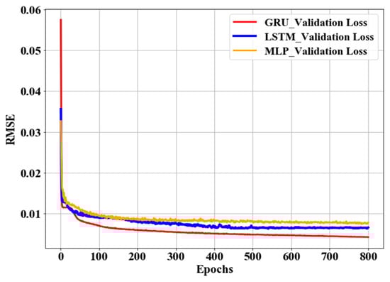
Figure 9.
Convergence of loss for GRU, LSTM, and MLP models. The plots show how the loss function decreased during training, indicating how well each model fit the data.
The superior performance of GRU in this study is due to its ability to capture long-term dependencies in input data. GRU has internal memories, allowing it to remember past inputs and incorporate them into current predictions. Such a capability is crucial for predicting ticket fares, as the pricing of tickets can be influenced by temporal factors such as the day of the week. GRU’s ability to capture these factors and incorporate them into predictions could result in more accurate fare predictions, as demonstrated by the lower root mean square error for the GRU model.
Additionally, GRU’s predictive power was compared with those of LSTM and MLP based on mean absolute error (MAE), root mean square error (RMSE), and coefficient of determination (R2), as presented in Table 6. As can be observed from Table 5, MLP was the worst in performance since it had the highest MAE and RMSE values and the lowest value of R2. The GRU model was superior in making accurate predictions, making it a reliable reference for the airline transport industry, both for travelers and aviators. The overall performance of GRU stands out as it surpassed both MLP and LSTM. When compared with MLP, the GRU model shows a decrease in MAE from 43.50 to 3.76, a decrease in RMSE from 64.93 to 5.93, and an increase in the coefficient of determination (R2) from 0.60 to 0.98. When compared to LSTM, the GRU model shows a decrease in MAE from 8.67 to 3.76, a decrease in RMSE from 13.99 to 5.93, and an increase in R2 from 0.70 to 0.98.
Table 6.
Performance comparison of the model prediction results.
Furthermore, the experimental results of two popular machine learning approaches, autoregressive integrated moving average (ARIMA) and support vector regression (SVR), are listed in Table 6 for comparison. ARIMA is a combination of the autoregressive model, which captures the dependency of the current observation output on the previous observations, and the moving average model, which captures the dependency on the current and previous inputs. The ARIMA model can be characterized as ARIMA (p, d, q), where p is the degree of autoregression, d is the degree of differencing, and q is the degree of moving average. In this study, we utilized the setting of ARIMA (5, 1, 1) to forecast future prices. In addition, for SVR, the kernel was set as a radial basis function (RBF). It can be observed from Table 6 that the GRU model stands out as a clear choice in fare prediction, providing the airline transport industry with a trustworthy reference.
Furthermore, the average of the predicted ticket fares for one flight based on the three different prediction models, GRU, LSTM, and MLP, were compared with the average of the actual fares in Table 7. The results in Table 7 indicate that the average of the predicted ticket fares for GRU is much closer to the actual average fares than those for LSTM and MLP. This suggests that GRU is a more accurate model for predicting ticket fares. Overall, the above results provide evidence of the superiority of the GRU model in predicting flight ticket fares and suggest that it is a promising approach for further study in this field.
Table 7.
Performance comparison of monthly averages for prediction models.
Figure 10, Figure 11, Figure 12 and Figure 13 further show the predicted and actual fares of all the flights for GRU, LSTM, MLP, and all three models, respectively, based on monthly averages. As can be observed from these figures, the predicted values by GRU were much closer to the actual values, as indicated by the lower absolute differences between the predicted and actual values. Given the extensive periods covered by historical flight prices, i.e., the four years and seven months in our dataset, the GRU model’s capabilities make it an appropriate choice for the fare prediction of flight tickets.
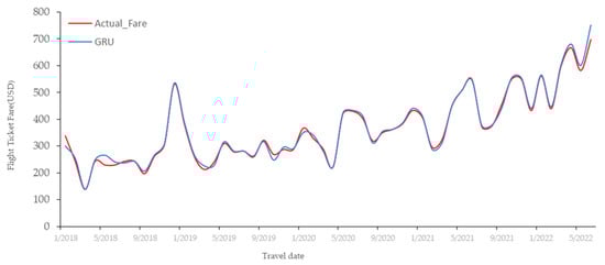
Figure 10.
Comparison of the actual values with the predictions obtained by the GRU model.
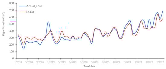
Figure 11.
Comparison of the actual values with the predictions obtained by the LSTM model.
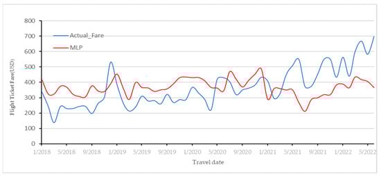
Figure 12.
Comparison of the actual values with the predictions obtained by the MLP model.
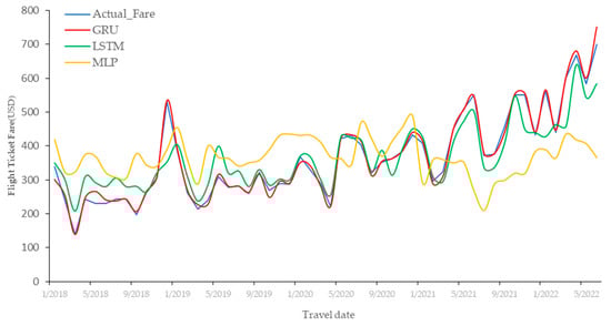
Figure 13.
Comparison of the actual values with the predictions obtained by the GRU, LSTM, and MLP models.
In addition, we conducted additional experiments with different prediction horizons to provide a comprehensive analysis of the model’s performance over varying timeframes. These experiments aimed to capture short-, medium-, and long-term forecasting scenarios. We evaluated the accuracy of the GRU model using three different prediction horizons; the time steps of 7, 14, and 30, and the experimental results are displayed in Figure 14. It can be observed from Figure 14 that the variations in the predicted outcomes for different prediction horizons were low, which demonstrates the robustness of the GRU model and provides valuable insights into the predictive capabilities of the model across different forecast periods.
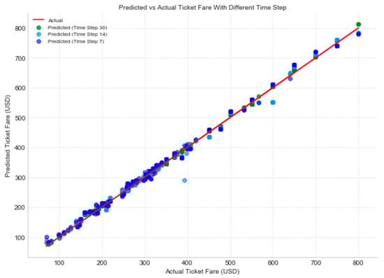
Figure 14.
Prediction of GRU model for different prediction horizons.
5. Conclusions
In this research, we have proposed using the GRU model as a solution for predicting airline ticket fares. Our analysis has demonstrated that this approach surpasses traditional neural networks in effectively preserving and leveraging historical datasets, resulting in more accurate and reliable predictions. This advancement represents a significant contribution to this field, and the straightforward architecture of the GRU model makes it highly practical and versatile for various applications.
However, it is imperative to acknowledge a crucial aspect that should be noticed. Forecasting the fare of an airline ticket is challenging due to the influence of a wide range of internal and external factors. These factors encompass social aspects, political dynamics, and even the market, which could be influenced by events in different countries. As a consequence, unexpected fluctuations in fare prices can occur. Future enhancements to the model should consider incorporating additional features not yet explored to address this complexity. It is essential to consider and account for such scenarios to further improve the predictive capabilities of the GRU model.
Furthermore, the scarcity of flying data in this domain highlights the importance of the work conducted on this deep-learning GRU model. The insights from this study pave the way for future research endeavors as they contribute to the development of more robust and comprehensive fare prediction models.
Author Contributions
W.A.D.: Conceptualization, Methodology, Software, Validation, Formal analysis, Investigation, Visualization, Writing—original draft. The final manuscript has been read and approved by both writers. B.-S.L.: Methodology, Conceptualization, Supervision, Resources, Writing—review & editing. All authors have read and agreed to the published version of the manuscript.
Funding
This research received no external funding.
Institutional Review Board Statement
Not applicable.
Informed Consent Statement
Not applicable.
Data Availability Statement
Not applicable.
Acknowledgments
We thank the Ethiopian Airline Headquarters in Addis Ababa, Ethiopia, for providing the flight ticket fare data for this research.
Conflicts of Interest
The authors declare no conflict of interest.
References
- Das, R.; Bo, R.; Chen, H.; Rehman, W.U.; Wunsch, D. Forecasting Nodal Price Difference Between Day-Ahead and Real-Time Electricity Markets Using Long-Short Term Memory and Sequence-to-Sequence Networks. IEEE Access 2022, 10, 832–843. [Google Scholar] [CrossRef]
- Jing, Y.; Guo, S.; Chen, F.; Wang, X.; Li, K. Dynamic Differential Pricing of High-Speed Railway Based on Improved GBDT Train Classification and Bootstrap Time Node Determination. IEEE Trans. Intell. Transp. Syst. 2022, 23, 16854–16866. [Google Scholar] [CrossRef]
- Wu, Y.; Cao, J.; Tan, Y.; Xiao, Q. A Data-Driven Agent-Based Simulator for Air Ticket Sales. In Computer Supported Cooperative Work and Social Computing; Springer: Berlin/Heidelberg, Germany, 2019; pp. 212–226. [Google Scholar]
- Yazdi, M.F.; Kamel, S.R.; Chabok, S.J.M.; Kheirabadi, M. Flight delay prediction based on deep learning and Levenberg-Marquart algorithm. J. Big Data 2020, 7, 1–28. [Google Scholar] [CrossRef]
- Bukhari, A.H.; Raja, M.A.Z.; Sulaiman, M.; Islam, S.; Shoaib, M.; Kumam, P. Fractional Neuro-Sequential ARFIMA-LSTM for Financial Market Forecasting. IEEE Access 2020, 8, 71326–71338. [Google Scholar] [CrossRef]
- Henrique, B.M.; Sobreiro, V.A.; Kimura, H. Literature review: Machine learning techniques applied to financial market prediction. Expert Syst. Appl. 2019, 124, 226–251. [Google Scholar] [CrossRef]
- Sahu, S.K.; Mokhade, A.; Bokde, N.D. An Overview of Machine Learning, Deep Learning, and Reinforcement Learning-Based Techniques in Quantitative Finance: Recent Progress and Challenges. Appl. Sci. 2023, 13, 1956. [Google Scholar] [CrossRef]
- Fayek, H.M.; Lech, M.; Cavedon, L. Evaluating deep learning architectures for Speech Emotion Recognition. Neural Netw. 2017, 92, 60–68. [Google Scholar] [CrossRef]
- Xiao, C.; Sutanto, D.; Muttaqi, K.M.; Zhang, M.; Meng, K.; Dong, Z.Y. Online Sequential Extreme Learning Machine Algorithm for Better Predispatch Electricity Price Forecasting Grids. IEEE Trans. Ind. Appl. 2021, 57, 1860–1871. [Google Scholar] [CrossRef]
- Minh, D.L.; Sadeghi-Niaraki, A.; Huy, H.D.; Min, K.; Moon, H. Deep Learning Approach for Short-Term Stock Trends Prediction Based on Two-Stream Gated Recurrent Unit Network. IEEE Access 2018, 6, 55392–55404. [Google Scholar] [CrossRef]
- Xu, X.; Zhang, Y. Soybean and Soybean Oil Price Forecasting through the Nonlinear Autoregressive Neural Network (NARNN) and NARNN with Exogenous Inputs (NARNN–X). Intell. Syst. Appl. 2022, 13, 200061. [Google Scholar] [CrossRef]
- Jianwei, E.; Ye, J.; Jin, H. A novel hybrid model on the prediction of time series and its application for the gold price analysis and forecasting. Phys. A Stat. Mech. Its Appl. 2019, 527, 121454. [Google Scholar] [CrossRef]
- Branda, F.; Marozzo, F.; Talia, D. Ticket Sales Prediction and Dynamic Pricing Strategies in Public Transport. Big Data Cogn. Comput. 2020, 4, 36. [Google Scholar] [CrossRef]
- Al Shehhi, M.; Karathanasopoulos, A. Forecasting hotel room prices in selected GCC cities using deep learning. J. Hosp. Tour. Manag. 2019, 42, 40–50. [Google Scholar] [CrossRef]
- Zhou, H.; Li, W.; Jiang, Z.; Cai, F.; Xue, Y. Flight Departure Time Prediction Based on Deep Learning. Aerospace 2022, 9, 394. [Google Scholar] [CrossRef]
- Meng, T.L.; Khushi, M. Reinforcement Learning in Financial Markets. Data 2019, 4, 110. [Google Scholar] [CrossRef]
- Ugurlu, U.; Oksuz, I.; Tas, O. Electricity Price Forecasting Using Recurrent Neural Networks. Energies 2018, 11, 1255. [Google Scholar] [CrossRef]
- Tanwar, S.; Patel, N.P.; Patel, S.N.; Patel, J.R.; Sharma, G.; Davidson, I.E. Deep Learning-Based Cryptocurrency Price Prediction Scheme With Inter-Dependent Relations. IEEE Access 2021, 9, 138633–138646. [Google Scholar] [CrossRef]
- Qi, L.; Khushi, M.; Poon, J. Event-Driven LSTM For Forex Price Prediction. In Proceedings of the 2020 IEEE Asia-Pacific Conference on Computer Science and Data Engineering (CSDE), Gold Coast, Australia, 16–18 December 2020; pp. 1–6. [Google Scholar]
- Hamayel, M.J.; Owda, A.Y. A Novel Cryptocurrency Price Prediction Model Using GRU, LSTM and bi-LSTM Machine Learning Algorithms. AI 2021, 2, 477–496. [Google Scholar] [CrossRef]
- Kim, G.I.; Jang, B. Petroleum Price Prediction with CNN-LSTM and CNN-GRU Using Skip-Connection. Mathematics 2023, 11, 547. [Google Scholar] [CrossRef]
- Subramanian, R.R.; Murali, M.S.; Deepak, B.; Deepak, P.; Reddy, H.N.; Sudharsan, R.R. Airline Fare Prediction Using Machine Learning Algorithms. In Proceedings of the 2022 4th International Conference on Smart Systems and Inventive Technology (ICSSIT), Tirunelveli, India, 20–22 January 2022; pp. 877–884. [Google Scholar]
- Guo, Y.; Han, S.; Shen, C.; Li, Y.; Yin, X.; Bai, Y. An Adaptive SVR for High-Frequency Stock Price Forecasting. IEEE Access 2018, 6, 11397–11404. [Google Scholar] [CrossRef]
- Abdella, J.A.; Zaki, N.M.; Shuaib, K.; Khan, F. Airline ticket price and demand prediction: A survey. J. King Saud Univ. Comput. Inf. Sci. 2021, 33, 375–391. [Google Scholar] [CrossRef]
- Chung, J.; Gulcehre, C.; Cho, K.; Bengio, Y. Empirical evaluation of gated recurrent neural networks on sequence modeling. arXiv 2014, arXiv:1412.3555. [Google Scholar]
- Chen, Y.; Cao, J.; Feng, S.; Tan, Y. An ensemble learning based approach for building airfare forecast service. In Proceedings of the 2015 IEEE International Conference on Big Data (Big Data), Santa Clara, CA, USA, 29 October–1 November 2015; pp. 964–969. [Google Scholar] [CrossRef]
- Lantseva, A.; Mukhina, K.; Nikishova, A.; Ivanov, S.; Knyazkov, K. Data-driven Modeling of Airlines Pricing. Procedia Comput. Sci. 2015, 66, 267–276. [Google Scholar] [CrossRef]
- Liu, Y.; Gong, C.; Yang, L.; Chen, Y. DSTP-RNN: A dual-stage two-phase attention-based recurrent neural network for long-term and multivariate time series prediction. Expert Syst. Appl. 2020, 143, 113082. [Google Scholar] [CrossRef]
- Liu, J.; Huang, X. Forecasting Crude Oil Price Using Event Extraction. IEEE Access 2021, 9, 149067–149076. [Google Scholar] [CrossRef]
- Busari, G.A.; Lim, D.H. Crude oil price prediction: A comparison between AdaBoost-LSTM and AdaBoost-GRU for improving forecasting performance. Comput. Chem. Eng. 2021, 155, 107513. [Google Scholar] [CrossRef]
- Zhang, Y.; Na, S. A Novel Agricultural Commodity Price Forecasting Model Based on Fuzzy Information Granulation and MEA-SVM Model. Math. Probl. Eng. 2018, 2018, 2540681. [Google Scholar] [CrossRef]
- Tuli, M.; Singh, L.; Tripathi, S.; Malik, N. Prediction of Flight Fares Using Machine Learning. In Proceedings of the 2023 13th International Conference on Cloud Computing, Data Science & Engineering (Confluence), Noida, India, 19–20 January 2023. [Google Scholar]
- Tziridis, K.; Kalampokas, T.; Papakostas, G.A.; Diamantaras, K.I. Airfare prices prediction using machine learning techniques. In Proceedings of the 2017 25th European Signal Processing Conference (EUSIPCO), Kos, Greece, 28 August–2 September 2017. [Google Scholar]
- Vu, V.H.; Minh, Q.T.; Phung, P.H. An airfare prediction model for developing markets. In Proceedings of the 2018 International Conference on Information Networking (ICOIN), Chiang Mai, Thailand, 10–12 January 2018. [Google Scholar]
- Prasath, S.N.; Eliyas, S. A Prediction of Flight Fare Using K-Nearest Neighbors. In Proceedings of the 2022 2nd International Conference on Advance Computing and Innovative Technologies in Engineering (ICACITE), Greater Noida, India, 28–29 April 2022; pp. 1347–1351. [Google Scholar]
- Al-Kwifi, O.S.; Frankwick, G.L.; Ahmed, Z.U. Achieving rapid internationalization of sub-Saharan African firms: Ethiopian Airlines’ operations under challenging conditions. J. Bus. Res. 2020, 119, 663–673. [Google Scholar] [CrossRef]
- Singh, G.; Singh, J.; Prabha, C. Data visualization and its key fundamentals: A comprehensive survey. In Proceedings of the 2022 7th International Conference on Communication and Electronics Systems (ICCES), Coimbatore, India, 22–24 June 2022. [Google Scholar]
- Wu, A.; Wang, Y.; Shu, X.; Moritz, D.; Cui, W.; Zhang, H.; Zhang, D.; Qu, H. AI4VIS: Survey on Artificial Intelligence Approaches for Data Visualization. IEEE Trans. Vis. Comput. Graph. 2021, 28, 5049–5070. [Google Scholar] [CrossRef]
- He, Z.; Zhou, J.; Dai, H.N.; Wang, H. Gold Price Forecast Based on LSTM-CNN Model. In Proceedings of the 2019 IEEE Intl Conference on Dependable, Autonomic and Secure Computing, Intl Conf on Pervasive Intelligence and Computing, Intl Conf on Cloud and Big Data Computing, Intl Conf on Cyber Science and Technology Congress (DASC/PiCom/CBDCom/CyberSciTech), Fukuoka, Japan, 5–8 August 2019; pp. 1046–1053. [Google Scholar]
- Chen, S.; Zhou, C. Stock Prediction Based on Genetic Algorithm Feature Selection and Long Short-Term Memory Neural Network. IEEE Access 2021, 9, 9066–9072. [Google Scholar] [CrossRef]
- Wang, D.; Fan, J.; Fu, H.; Zhang, B. Research on Optimization of Big Data Construction Engineering Quality Management Based on RNN-LSTM. Complexity 2018, 2018, 1–16. [Google Scholar] [CrossRef]
- Jovanovic, L.; Jovanovic, D.; Bacanin, N.; Stakic, A.J.; Antonijevic, M.; Magd, H.; Thirumalaisamy, R.; Zivkovic, M. Multi-Step Crude Oil Price Prediction Based on LSTM Approach Tuned by Salp Swarm Algorithm with Disputation Operator. Sustainability 2022, 14, 14616. [Google Scholar] [CrossRef]
- Li, C.; Qian, G. Stock Price Prediction Using a Frequency Decomposition Based GRU Transformer Neural Network. Appl. Sci. 2022, 13, 222. [Google Scholar] [CrossRef]
- Zhu, D.; Wang, Y.; Zhang, F. Energy Price Prediction Integrated with Singular Spectrum Analysis and Long Short-Term Memory Network against the Background of Carbon Neutrality. Energies 2022, 15, 8128. [Google Scholar] [CrossRef]
- Yurtsever, M. Gold Price Forecasting Using LSTM, Bi-LSTM and GRU. Eur. J. Sci. Technol. 2021, 31, 341–347. [Google Scholar] [CrossRef]
- Dehnaw, A.M.; Manie, Y.C.; Chen, Y.Y.; Chiu, P.H.; Huang, H.W.; Chen, G.W.; Peng, P.C. Design Reliable Bus Structure Distributed Fiber Bragg Grating Sensor Network Using Gated Recurrent Unit Network. Sensors 2020, 20, 7355. [Google Scholar] [CrossRef]
- Tolosana, R.; Vera-Rodriguez, R.; Fierrez, J.; Ortega-Garcia, J. Exploring Recurrent Neural Networks for On-Line Handwritten Signature Biometrics. IEEE Access 2018, 6, 5128–5138. [Google Scholar] [CrossRef]
- Deng, Y.; Wang, L.; Jia, H.; Tong, X.; Li, F. A Sequence-to-Sequence Deep Learning Architecture Based on Bidirectional GRU for Type Recognition and Time Location of Combined Power Quality Disturbance. IEEE Trans. Ind. Inform. 2019, 15, 4481–4493. [Google Scholar] [CrossRef]
- Zhang, S.; Luo, J.; Wang, S.; Liu, F. Oil price forecasting: A hybrid GRU neural network based on decomposition–reconstruction methods. Expert Syst. Appl. 2023, 218, 119617. [Google Scholar] [CrossRef]
- Willmott, C.J.; Matsuura, K. Advantages of the mean absolute error (MAE) over the root mean square error (RMSE) in assessing average model performance. Clim. Res. 2005, 30, 79–82. [Google Scholar] [CrossRef]
- Zhang, D. A Coefficient of Determination for Generalized Linear Models. Am. Stat. 2017, 71, 310–316. [Google Scholar] [CrossRef]


Disclaimer/Publisher’s Note: The statements, opinions and data contained in all publications are solely those of the individual author(s) and contributor(s) and not of MDPI and/or the editor(s). MDPI and/or the editor(s) disclaim responsibility for any injury to people or property resulting from any ideas, methods, instructions or products referred to in the content. |
© 2023 by the authors. Licensee MDPI, Basel, Switzerland. This article is an open access article distributed under the terms and conditions of the Creative Commons Attribution (CC BY) license (https://creativecommons.org/licenses/by/4.0/).