Abstract
Video Snapshot Compressive Imaging (SCI) is a new imaging method based on compressive sensing. It encodes image sequences into a single snapshot measurement and then recovers the original high-speed video through reconstruction algorithms, which has the advantages of a low hardware cost and high imaging efficiency. How to construct an efficient algorithm is the key problem of video SCI. Although the current mainstream deep convolution network reconstruction methods can directly learn the inverse reconstruction mapping, they still have shortcomings in the representation of the complex spatiotemporal content of video scenes and the modeling of long-range contextual correlation. The quality of reconstruction still needs to be improved. To solve this problem, we propose a Transformer-based Cascading Reconstruction Network for Video Snapshot Compressive Imaging. In terms of the long-range correlation matching in the Transformer, the proposed network can effectively capture the spatiotemporal correlation of video frames for reconstruction. Specifically, according to the residual measurement mechanism, the reconstruction network is configured as a cascade of two stages: overall structure reconstruction and incremental details reconstruction. In the first stage, a multi-scale Transformer module is designed to extract the long-range multi-scale spatiotemporal features and reconstruct the overall structure. The second stage takes the measurement of the first stage as the input and employs a dynamic fusion module to adaptively fuse the output features of the two stages so that the cascading network can effectively represent the content of complex video scenes and reconstruct more incremental details. Experiments on simulation and real datasets show that the proposed method can effectively improve the reconstruction accuracy, and ablation experiments also verify the validity of the constructed network modules.
1. Introduction
Signal sampling is the first prerequisite for signal processing and analysis. The compressive sensing theory [1,2,3,4,5] points out that sparse signals or signal sparse in the transform domain can be recovered from much less compressed measurements than the Nyquist sampling. It is a more efficient signal sensing method, which can realize the synchronous compression of signals during the sampling process.
In recent years, a variety of new computational imaging methods based on compressive sensing theory have emerged [6,7]. The Coded Aperture Compressive Temporal Image (CACTI) is one of the representative methods. As shown in Figure 1, this imaging mode first modulates the video scene (image sequence) through different masks and then integrates and accumulates along the time dimension to form a single-frame snapshot measurement, which is finally captured by a two-dimensional detector. Video snapshot compressive imaging modulates and compresses the video sequences in the time dimension, which can reduce the burden of data storage and the requirements of the transmission bandwidth. Since the snapshot measurement is encoded and compressed information, it is necessary to design an efficient reconstruction algorithm to recover the original video, which is an important factor affecting the quality of video snapshot compressive imaging.
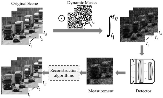
Figure 1.
Schematic diagram of video snapshot compressive imaging.
The existing reconstruction algorithms are mainly divided into two categories: iterative optimization-based methods and deep network-based methods. The iterative optimization methods [8,9,10,11,12,13,14] formulate the reconstruction process as a variational problem with a priori regularization constraints and solve it through the optimization algorithm iteratively. Total variation, the Gaussian mixture model and non-local low rank are widely used prior regularization constraints. However, these hand-crafted models cannot represent complex and dynamic scene content in videos effectively, which degrades the reconstruction quality. At the same time, this category of methods involves multiple iterations, and each iteration needs to solve the proximal operator of the priori regularization constraint [13], which has a high computational complexity and long reconstruction time. For example, the DeSCI method [8] used nonlocal low rank as a priori to improve the reconstruction quality, but it takes about 1 h to recover eight frames from the measurement.
Inspired by the successful application of the deep network model in computer vision tasks, scholars have also applied the deep network to snapshot compressive imaging tasks [15,16,17,18,19,20,21]. Their main idea is to design a network to directly learn the inverse mapping from the snapshot measurement to the original signal. Unlike the iterative optimization solution, the original video can be quickly reconstructed without iteration by inputting the snapshot measurement into the trained reconstruction networks. At present, the mainstream reconstruction networks mainly use the convolution neural network to extract features for reconstruction. However, the size of the convolution kernel is usually small, so they can only extract local features. Although stacking multiple convolutions can improve the receptive field range of deep features, it still cannot capture the long-range spatiotemporal correlation in image sequences, affecting the reconstruction quality.
How to represent the video dynamic scene content effectively, especially how to make use of long-range spatiotemporal correlation, is the key to improving the reconstruction quality. Transformer [22,23,24,25,26,27,28,29,30], as a novel network architecture, uses a self-attention mechanism to represent long-term relations and has shown excellent performance in visual tasks. Therefore, we introduce Transformer into the task of video snapshot compressive imaging and propose a Transformer-based Cascading Reconstruction Network. The proposed network exploits both the ability of the local feature extraction of the convolution kernel and the capacity of capturing the global context information of the Transformer to learn the spatiotemporal characteristics of video scenes. Meanwhile, considering the complexity of a video scene, according to the residual measurement mechanism [31], the proposed network is designed as two cascading stages: overall structure reconstruction and incremental details reconstruction. In the first stage, the multi-scale Transformer network is designed to reconstruct the overall structure by extracting multi-scale and long-range spatiotemporal features. In the second stage, the measurement residual of the first stage is taken as the input, and the dynamic fusion Transformer network is designed to adaptively fuse the features of the Transformer in the two stages so as to reconstruct incremental details. In this way, more detailed structures can be reconstructed, and the reconstruction quality can be effectively improved. The main contributions of our work are as follows:
- (1)
- We propose a Transformer-based Cascading Reconstruction Network to learn multi-scale and long-range spatiotemporal features for video snapshot compressive imaging. The cascading network architecture can also improve the network’s ability to effectively represent the content of complex video scenes effectively.
- (2)
- In order to coordinate the two stages better, we propose a dynamic fusion Transformer to adaptively fuse the features of the two stages so that the second stage can reconstruct more incremental details.
- (3)
- Experiments on simulated and real datasets show that the proposed network can improve the reconstruction quality significantly, and the ablation studies also verify the effectiveness of our network architecture.
2. Related Works
Video snapshot compressive imaging includes two stages: compressive encoding and decoding reconstruction. This section introduces the encoding model of video snapshot compressive imaging, then summarizes two categories of decoding and reconstruction methods and, finally, summarizes the vision Transformer briefly.
2.1. Video Compressive Snapshot Imaging
We denote the dynamic scene with frame images as , where and are the spatial sizes. The CACTI system [7] uses the mask matrices to modulate the frame sequence of the dynamic scene. Then, the modulated frames are accumulated on the sensor array to obtain the final single-frame measurement . The imaging process of the CACTI system can be mathematically expressed as
where is the measurement noise and denotes the Hadamard (element-wise) multiplication. According to Equation (1), each entry in the snapshot measurement is calculated as
The pixels at position of each modulated frame are collapsed to form one pixel in the snapshot measurement. We can also summarize the forward imaging process of the CACTI system as a concise matrix equation,
In Equation (3), is the sensing matrix, and is the vectorized image sequence, where and vectorize the matrix by stacking columns. denotes the vectorized noise. The sensing matrix in (3) can be written as
where are diagonal matrices, and reshapes the vector into a diagonal matrix by taking the vector as its main diagonal.
In the imaging process of the CACTI system, the original video is compressed into one frame with a compression rate of . At present, coded modulation in the CACTI system is mainly realized by a digital micromirror device (DMD) [32,33,34] and code matrix shifting. For example, DMD is composed of many small aluminum mirrors. It can code and modulate the object by turning each mirror at a high speed. The literature [35] modulated the high-speed video frames by shifting the same coding matrix.
2.2. Reconstruction Methods
Video snapshot compressive imaging is a computational imaging method that requires decoding to reconstruct the original video scenes. The reconstruction method is the key to affect the quality of SCI imaging. The classical variational methods mainly use the structural prior as the regular term to construct models. GMM-TP [11] used the Gaussian mixture model to represent video scenes and estimated the parameters of the Gaussian mixture model through the expectation maximization algorithm. MMLE-GMM [9] used the maximum boundary likelihood estimator to learn the distribution parameters from measurements. GAP-TV [13] used the total variation regularization as a prior constraint and solved the problem by the generalized alternating projection algorithm. DeSCI [8] used the weighted kernel norm minimization to capture the low-rank structure of video patches. However, the models mentioned above need to be solved iteratively with high complexity.
Recently, researchers have applied deep networks to SCI tasks by training the network to learn the mapping from training datasets to original signals. Then, the fast reconstruction can be achieved by inputting the measurements of video into the trained network. The key problem of such methods is the design of a reconstruction network. A codec structure network was proposed in [18], which represented the inverse mapping from the measurement to the reconstruction result. Yuan et al. expanded the iterative optimization model into a network module based on the generalized alternating projection and alternating direction multiplier method and used different deep denoisers as a prior constraint to form a plug-and-play reconstruction network model (PnP-FFDNet) [17]. Sun et al. proposed the residual integration network RE2-Net [19], which consisted of four subnets of different structures to capture the temporal and spatial correlation between frames to reconstruct video scenes. Huang et al. proposed a multi-hypothesis motion compensation structure [20], which can exploit the similarity between neighboring frames to improve the reconstruction quality. Although the existing network models based on convolutional operations can effectively extract local features, there are still shortcomings in capturing global context information and modeling complex video scenes, and the reconstruction quality needs to be further improved.
2.3. Vision Transformer
Transformer [22] is a classic model in natural language processing. The correlation between different texts is calculated through global matching, which improves the network’s ability to learn the long range of association features. According to its excellent performance, Transformer has also been widely used in computer vision tasks such as image segmentation, image classification, object detection, etc.
Alexey et al. proposed Vision Transformer (ViT) [25] for the first time, which decomposed the image into block sequences and input them as Tokens into the attention module for correlation calculation, which can extract the long-range features of the image and achieve excellent performance in classification tasks. Liu et al. proposed Swin Transformer [26], which limited multi-head self-attention computation in non-overlapping local windows to improve computational efficiency. This method achieved cross-window information interaction through window shifting, which made it compatible with different visual tasks. Liu et al. followed the hierarchical structure of the original Swin Transformer, expanding the scope of local attention calculation from the spatio domain to the spatiotemporal domain [27]. Liang et al. proposed SwinIR [28] on the basis of Swin Transformer. This model had improved performance in image reconstruction, super-resolution and other tasks by using sets of residual Swin Transformer modules. Cui et al. proposed the Meta-TR model in [29]. The model used Swin Transformer as a backbone and designed a meta-attention module, which converted the sensing matrix into an attention vector to guide the training of the compressive sensing reconstruction network and achieved a good balance in reconstruction performance, model parameter quantity and running time. Saidini et al. [30] replaced the full connection layer in the multi-head attention with the convolution layer to make better use of remote spatiotemporal correlations.
Transformer has shown excellent performance in reconstruction tasks and computer vision problems. Therefore, we introduce Transformer into video snapshot compressive imaging tasks and propose a Cascading Reconstruction Network to achieve high-quality reconstruction.
3. Transformer-Based Cascading Reconstruction Network
We propose a Transformer-based Cascading Reconstruction Network for learning the explicit reconstruction mapping. As shown in Figure 2, the proposed network takes the snapshot measurement as the input and cascades two stages to realize reconstruction. Ahead of the two stages, we first calculate the initial reconstruction from the input measurement , which can be expressed as
where , is the Hadamard (element-wise) division and is the integral of masks. The initial reconstruction calculated by Equation (5) can contain more scene background information [15] and is then input to the overall structure reconstruction network for subsequent processing.
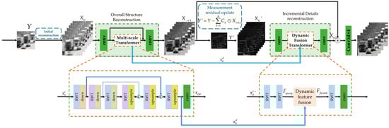
Figure 2.
The diagram of the Transformer-based Cascading Reconstruction Network for Video Compressive Snapshot Imaging.
By taking the as the input, the first stage is to reconstruct the overall structures of the original video through the multi-scale Transformer module. According to the residual measurement mechanism, we can obtain the updated residual measurement . The second stage fuses the features of two stages to reconstruct the incremental details features. The final reconstructed video is obtained by combining the two-stage reconstruction.
3.1. Overall Structure Reconstruction
The overall structure reconstruction stage is designed as a multi-scale Transformer network with an encoder and decoder for extracting multi-scale and long-range spatiotemporal features from the initial reconstruction. Figure 3 shows the diagram of the multi-scale Transformer network. The encoder and decoder are also linked with skip connection.
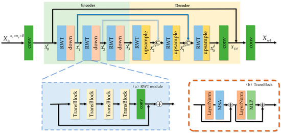
Figure 3.
The diagram of the multi-scale Transformer network for overall structure reconstruction.
The encoder first employs a convolution layer to adjust the number of channels of and outputs the feature map with channels. The encoder has three scales, and each scale is configured with the Residual Window Transformer (RWT) module and the down-sampling operation. The processing of each scale can be defined as
where , , , represents the -th down-sampling and denotes the deep feature extraction mapping of the RWT module.
Each RWT module contains a residual link, four TransBlocks and one convolution layer. TransBlock adopts non-overlapping local window attention in TransBlock, as in [26]. In detail, we divide the input feature maps of size into non-overlapping local windows of size . Therefore, there are a total of windows. Then, we calculate the correlations in each window through the self-attention mechanism. The features of the local window are reshaped into tokens . With the embedding projection, the Query, Key and Value matrices can be calculated as
where represent the projection matrices, and they are shared across different windows. After that, we can calculate the self-attention matrix of each local window and update the features as
where denotes the learnable positional encoding. TransBlock uses Window Multi-head Self-Attention (W-MSA) to calculate self-attentions in parallel and concatenates the results of multi-head. In addition, the outputs of W-MSA undergo the processing of Multi-Layer Perception (MLP) and the LayerNorm (LN) layer. Two residual connections are used inside TransBlock. The whole calculation formula of TransBlock is as follows:
where represents the -th output of TransBlock.
The decoder has a structure symmetry with the encoder. Each scale of the decoder is configured with an RWT module and an up-sampling operation. The features of the same scale in the encoder are transmitted to the decoder through a skip connection and a concatenation operation. The calculation of each scale in the decoder can be written as
where , and . represents the up-sampling, denotes a convolution layer that reduce the number of channels from to . Through hierarchical decoding, we can obtain the deep features . With the global residual link, we can obtain the overall structure reconstruction , which is computed as
3.2. Measurement Residual Update
According to the residual measurement mechanism [31], we update the measurements’ residual and input it into the second stage to complete the recovery of incremental details. Specifically, the output of the first stage is modulated with the same mask according to the forward model of the CACTI system. Then, we subtract it from the original measurement to obtain the measurement residual , which is computed as
The measurement residual can be regarded as the measurement of the remaining image details apart from the overall structure reconstruction. Therefore, the second stage can utilize it to reconstruct the incremental details.
3.3. Incremental Details Reconstruction
The incremental details reconstruction stage is designed as a dynamic fusion Transformer network to further improve the reconstruction quality. Figure 4 shows its network architecture. In order to better coordinate the two reconstruction stages, we design a dynamic feature fusion module to adaptively fuse the features of the two stages. The final reconstruction can be obtained by combining the incremental details and the overall structure reconstruction.
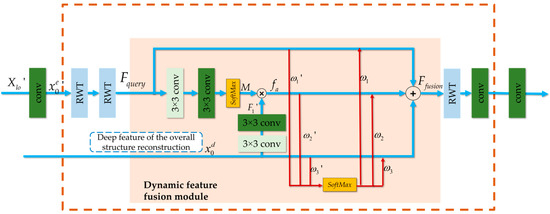
Figure 4.
The diagram of the dynamic fusion Transformer network for incremental details reconstruction.
The dynamic feature fusion module integrates the Transformer features of two stages into three branches and performs adaptive fusion. The first branch calculates the initial reconstruction from and then performs the operations of a convolution and two RWT modules on to obtain the intermediate feature . The third branch accepts the deep feature from the first stage. The second branch calculates an attention map from through the operations of two convolutions and one and obtains a complementary feature by gating between and the attention map , where is obtained from through the operations of two convolution layers. The fusion weights of the three branches are learned adaptively by the network, which is helpful in promoting the two-stage network to reconstruct more incremental details. The core fusion operations can be formulated as
where represents the convolution of 3 × 3, the function in the module is to normalize into a probability distribution map or normalize the parameter . is the fused feature.
After performing the operations of one RWT module and two convolutions upon , we can obtain the incremental reconstruction . Then, the incremental reconstruction is summed up with the overall structure reconstruction .
After four 3D convolution layers, the final reconstruction result is calculated as
4. Network Parameters Learning
We train the proposed network in an end-to-end way and define the loss function to guide the network parameters learning, which is defined below:
where is the final output of the reconstruction network, is the ground-truth and is the overall structure reconstruction results; is an anisotropic total variation constraint, both and are regularization parameters. In the first term of the loss function, we use mean square error (MSE) loss to require the final output of the network to approximate the ground-truth. The total variation constraint term can restrain each frame of the reconstruction results to have bounded variation [13], which can effectively preserve the overall structure. Therefore, we use mean square error loss in the second term and the total variation constraint in the third term to require the output of the overall structure reconstruction to satisfy the total variation prior constraint while approximating the ground-truth. We also use and as the hyperparameters to weight both the terms. The network learning algorithm is shown in Algorithm 1.
| Algorithm 1: Transformer-based Cascading Reconstruction Network. |
| input: learning rate , batch size , maximal iteration number , regularization parameter , , measurement matrix |
| output: network parameter |
|
5. Experiment Results and Analysis
In this section, we compare the proposed network with several state-of-the-art methods on both the simulation datasets and the real dataset. Meanwhile, ablation studies are conducted to verify the effectiveness of our network design.
5.1. Datasets and Experimental Setting
Following the dataset used in [18], we choose the DAVIS2017 dataset [36] as the training set of the proposed network. The DAVIS2017 dataset has 90 different scenes and a total of 6208 frames with two resolutions: 480 × 894 and 1080 × 1920. These video scenes are cut into video cubes of 8 × 256 × 256. Then, we use the binary random masks used in [18] to modulate these eight consecutive frames () into one frame snapshot measurement according to Equation (1). The compression ratio of the binary random mask is 50%. In this way, the original video is compressed into one frame at a compression rate of 1/8, and each frame is modulated with a 50% ratio. We group each video cube and corresponding snapshot measurement into a data pair and collect 13,000 data pairs as the training set. We test the trained reconstruction network on both the simulation datasets and the real dataset. The simulation datasets contain Kobe, Traffic, Runner, Drop [8], Crash and Aerial [17]. We adopt the same setting as in the training set to generate the snapshot measurements. The real data Wheel [7] is captured by the SCI camera. We use PyTorch to train the proposed network on the RTX 3090 GPU and use the Adam optimizer [37] to minimize the loss function. The initial learning rate is 2 × 10⁻⁴ and we reduce the learning rate by 10% every 10 epochs. The epoch number is set as 100. The values of the hyper parameters and of Equation (20) are both set as 1 × 10⁻¹.
5.2. Results on Simulation Datasets
In this section, we compare the proposed network with several representative methods, including the iterative optimization-based methods GAP-TV [13], GMM-TP [11], MMLE-MFA [9] and MMLE-GMM [9] and four deep learning-based methods, including the plug-and-play methods PnP-FFDNet [17], E2E-CNN [18], RE2-Net [19] and Saideni’s algorithm [30]. We use the peak-signal-to-noise ratio (PSNR) and structural similarity (SSIM) [38] as metrics to evaluate the reconstruction quality.
The PSNR and SSIM of each method are listed in Table 1. The GAP-TV method uses total variation as the prior regularization, and its PSNR and SSIM values are the lowest. Both GMM-TP and MMLE-GMM use the Gaussian mixture model as the prior regularization. The performance of MMLE-GMM is better than that of GMM-TP. MMLE-MFA is a simplified model of MMLE-GMM, and its reconstruction performance is lower than that of MMLE-GMM. PnP-FFDNet, E2E-CNN, Saideni’s algorithm and RE2-Net are deep learning-based methods, and their reconstruction qualities are generally higher than the traditional iterative optimization-based methods. RE2-Net learns the spatiotemporal correlation through network ensemble and has the second-best results. Saideni’s algorithm uses Transformer to capture long-range spatiotemporal features and has the best reconstruction on the Kobe and Aerial datasets. However, the average results of Saideni ’s algorithm are lower than those in our network. The proposed network has the optimal reconstruction quality in Runner and Drop and achieves the optimal average PSNR and SSIM values among all the methods. Figure 5 shows the reconstruction results of two stages in our network, including the overall structure reconstruction, the incremental details reconstruction and the final reconstruction. It can be seen that the second stage can reconstruct informative incremental details and further enhance the quality of the final reconstruction, which verifies the rationality of our cascading network design. The advantages of our network mainly lie in three aspects. First, the proposed network adopts the multi-scale Transformer structure to fully extract the overall spatial and temporal correlation of video frames. Second, according to the residual measurement mechanism, we decompose the reconstruction as the cascading of the overall structure reconstruction and the incremental details reconstruction, which helps to reduce the learning difficulty of the network. Lastly, the dynamic feature fusion module can adaptively fuse the reconstruction of two stages and reconstruct more incremental details.

Table 1.
The PSNR in dB (left entry) and SSIM (right entry) metrics of different methods on six simulation datasets. The optimal results are shown in bold, and the second-best results are underlined.
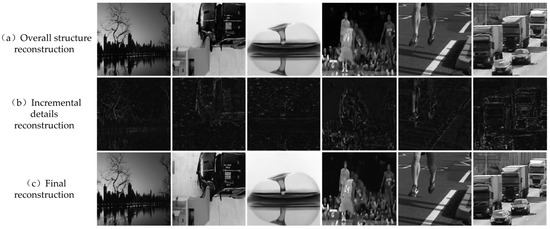
Figure 5.
The reconstruction results of two stages in our network: (a) Overall structure reconstruction; (b) Incremental details reconstruction; (c) Final reconstruction.
Figure 6 shows the reconstructed video frames of different methods on the simulation datasets. The leftmost column is Ground Truth, and the rightmost is the result of our network. It can be seen from Figure 5 that the video frames reconstructed by GMM-TP, MMLE-MFA and MMLE-GMM have a relatively blurry contour, and there are artifacts in the reconstruction. PnP-FFDNet, E2E-CNN and RE2-Net make some improvements on the contour reconstruction, but they still lack structural details in reconstruction frames. The proposed network can effectively reconstruct the contour structures and detail information of the objects, and it has the best visual quality.
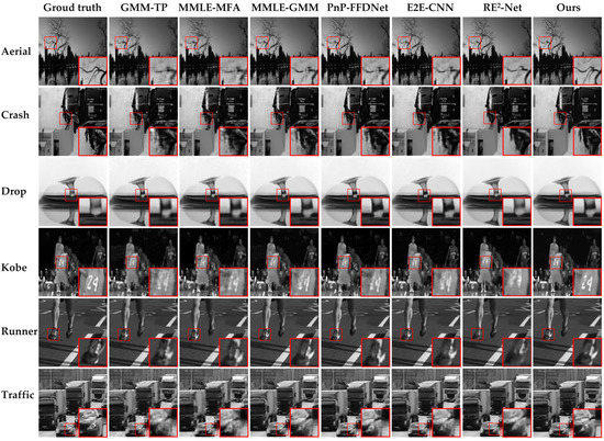
Figure 6.
Reconstructed frames of six simulation datasets by different methods (the left side is the Ground Truth, and the right side is the reconstruction result of each method). The sequence numbers of the selected frames of each dataset are Aerial #5, Crash #24, Drop #4, Kobe #6, Runner #1 and Traffic #18.
5.3. Results on Real Datasets
In this section, we apply the proposed network on the real data Wheel captured by the SCI camera [7]. The size of the measurement is 256 × 256, which is obtained by encoding every 14 frames by shifting binary random masks. Due to the lack of corresponding original video, we cannot calculate the evaluation metrics and instead evaluate the visual quality of the reconstructed videos. Figure 7 shows the reconstruction results of the proposed network, E2E-CNN, GAP-TV and RE2-Net for the Wheel dataset. It can be observed that the results of the proposed network can obtain sharper edges of the letter “D” and a clearer scene. There are some artifacts in the reconstructions of GAP-TV and RE2-Net. The reconstruction results of E2E-CNN have less accurate motion information and contour details.
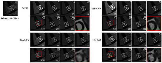
Figure 7.
Reconstruction results of different methods on the real dataset Wheel. (The red boxes are enlarged detail images.)
5.4. Ablation Studies
In this section, we take a series of ablation experiments to understand the impact of the performance of the different parts of the proposed network. We design ablation methods by removing some modules from the proposed network. The ablation methods 1–3 are to verify the effectiveness of the residual measurement mechanism and dynamic feature fusion module. The ablation methods 4–7 modify the group number of the multi-scale structure in the overall structure reconstruction network and the number of RWT modules in the incremental details reconstruction stage. Table 2 demonstrates the detailed setting of seven ablation methods and their experimental results on the simulation datasets.
Table 2.
Ablation results of the proposed network.
In ablation methods 2 and 3, the removing of the residual measurement mechanism means that we directly take the output of the overall structure reconstruction network as the input of the incremental details network. In ablation methods 1 and 3, the removing of the dynamic feature fusion module means that the second stage only takes the output of the first stage as the input instead of fusing it with the deep feature captured by the first stage. In these three experiments, one or two modules are removed, respectively, and the rest of the network maintains the original structure. As shown in Table 2, removing any module will reduce the reconstruction quality. This proves that the residual measurement mechanism and dynamic feature fusion module can make the network focus more on the recovery of details, effectively enhancing the learning ability of the network and improving the reconstruction quality.
In ablation experiments 4–7, we change both the group number of the multi-scale structure in the overall structure reconstruction network and the number of RWT modules in the incremental details reconstruction network. In the proposed network, the overall structure reconstruction network includes three groups of multi-scale structures. As shown in Table 2, with the group number of the multi-scale structure decreasing, the PSNR is reduced from 32.42 dB to 31.16 dB, which proves the effectiveness of the RWT module. When the overall structure reconstruction network is kept unchanged and the number of RWT modules in the detail reconstruction network is reduced, the quality of reconstruction will be reduced, which also proves the effectiveness of this module for the proposed network.
5.5. Time Complexity and Parameter Quantity
Both time complexity and parameter quantity are important aspects of evaluating video SCI. We run our network, E2E-CNN and RE2-Net on GPU and run PnP-FFDNet on MATLAB. The other traditional iterative optimization-based methods are run on CPU. Table 3 compares the average running time required by different methods to reconstruct six simulation datasets and the quantity of parameters of deep network-based methods. The reconstruction time, reconstruction frames per second (FPS) and parameters quantity for different methods are respectively listed in the table. The reconstruction time of GAP-TV, GMM-TP, MMLE-MFA and MMLE-GMM is much longer than that of methods based on a deep network. The proposed network takes 6.7346 s to reconstruct a video dataset, and the FPS is 4.7516. Although the reconstruction time of the proposed network is longer than that of RE2-Net and E2E-CNN, it has a lower parameters quantity than RE2-Net and a better reconstruction quality than E2E-CNN. It can be seen that the proposed network achieves a good balance between the complexity of the model and the reconstruction speed while improving the reconstruction quality at a reasonable computational cost.
Table 3.
Comparison of the reconstruction time of different methods.
6. Conclusions
We propose a Transformer-based cascading reconstruction network for video snap-shot compressive imaging. The network is configured as a cascade of two stages: overall structure reconstruction and incremental details reconstruction. In the first stage, a multi-scale Transformer network is designed to extract the multi-scale spatiotemporal features, and the residual measurement mechanism is used to calculate the measurement residual of the reconstruction of the first stage. The incremental details reconstruction network takes the measurement residual as the input and utilizes the dynamic feature fusion module to adaptively fuse the output features of the two stages to improve the reconstruction quality. Experiments show that the proposed network effectively utilizes the advantages of the Transformer and the convolution neural network. Compared with the current reconstruction methods based on convolution neural networks, the proposed network can obtain better reconstruction quality.
Author Contributions
J.W.: investigation, resources, methodology, writing—original draft. J.H.: software, validation. X.C.: formal analysis, data curation. K.H.: visualization. Y.S.: conceptualization, writing—review and editing, supervision, funding acquisition. All authors have read and agreed to the published version of the manuscript.
Funding
This research was funded by The National Natural Science Foundation of China under Grant U2001211 and 62276139.
Institutional Review Board Statement
Not applicable.
Informed Consent Statement
Not applicable.
Data Availability Statement
The data are available at https://github.com/bonjourcc/TBC-SCINet/tree/main (accessed on 8 May 2023).
Conflicts of Interest
The authors declare no conflict of interest.
References
- Donoho, D.L. Compressed sensing. IEEE Trans. Inf. Theory 2006, 52, 1289–1306. [Google Scholar] [CrossRef]
- Chen, S.S.; Donoho, D.L.; Saunders, M.A. Atomic decomposition by basis pursuit. SIAM Rev. 2001, 43, 129–159. [Google Scholar] [CrossRef]
- Candès, E.J.; Romberg, J.K.; Tao, T. Stable signal recovery from incomplete and inaccurate measurements. Commun. Pure Appl. Math. J. Issued Courant Inst. Math. Sci. 2006, 59, 1207–1223. [Google Scholar] [CrossRef]
- Candès, E.J.; Romberg, J.K.; Tao, T. Robust uncertainty principles: Exact signal reconstruction from highly incomplete frequency information. IEEE Trans. Inf. Theory 2006, 52, 489–509. [Google Scholar] [CrossRef]
- Li, L.; Fang, Y.; Liu, L.; Peng, H.; Kurths, J.; Yang, Y. Overview of Compressed Sensing: Sensing Model, Reconstruction Algorithm, and Its Applications. Appl. Sci. 2020, 10, 5909. [Google Scholar] [CrossRef]
- Jalali, S.; Yuan, X. Snapshot compressed sensing: Performance bounds and algorithms. IEEE Trans. Inf. Theory 2019, 65, 8005–8024. [Google Scholar] [CrossRef]
- Llull, P.; Liao, X.; Yuan, X.; Yang, J.; Kittle, D.; Carin, L.; Sapiro, G.; Brady, D.J. Coded aperture compressive temporal imaging. Opt. Express 2013, 21, 10526–10545. [Google Scholar] [CrossRef]
- Liu, Y.; Yuan, X.; Suo, J.; Brady, D.J.; Dai, Q. Rank minimization for snapshot compressive imaging. IEEE Trans. Pattern Anal. Mach. Intell. 2018, 41, 2990–3006. [Google Scholar] [CrossRef]
- Yang, J.; Liao, X.; Yuan, X.; Llull, P.; Brady, D.J.; Sapiro, G.; Carin, L. Compressive sensing by learning a Gaussian mixture model from measurements. IEEE Trans.-Ions Image Process. 2014, 24, 106–119. [Google Scholar] [CrossRef]
- Krahmer, F.; Kruschel, C.; Sandbichler, M. Total variation minimization in compressed sensing. In Compressed Sensing and Its Applications; Birkhäuser: Cham, Switzerland, 2017; pp. 333–358. [Google Scholar]
- Yang, J.; Yuan, X.; Liao, X.; Llull, P.; Brady, D.J.; Sapiro, G.; Carin, L. Video compressive sensing using Gaussian mixture models. IEEE Trans. Image Process. 2014, 23, 4863–4878. [Google Scholar] [CrossRef]
- Ma, J.; Liu, X.Y.; Shou, Z.; Yuan, X. Deep tensor admm-net for snapshot compressive imaging. In Proceedings of the IEEE/CVF International Conference on Computer Vision, Seoul, Korea, 27 October–2 November 2019; pp. 10223–10232. [Google Scholar]
- Yuan, X. Generalized alternating projection based total variation minimization for compressive sensing. In Proceedings of the International Conference on Image Processing (ICIP), Phoenix, AZ, USA, 25 September 2016; pp. 2539–2543. [Google Scholar]
- Wei, Z.; Zhang, J.; Xu, Z.; Liu, Y. Optimization Methods of Compressively Sensed Image Reconstruction Based on Single-Pixel Imaging. Appl. Sci. 2020, 10, 3288. [Google Scholar] [CrossRef]
- Cheng, Z.; Chen, B.; Liu, G.; Zhang, H.; Lu, R.; Wang, Z.; Yuan, X. Memory-efficient network for large-scale video compressive sensing. In Proceedings of the IEEE/CVF Conference on Computer Vision and Pattern Recognition, Nashville, TN, USA, 20–25 June 2021; pp. 16246–16255. [Google Scholar]
- Saideni, W.; Helbert, D.; Courreges, F.; Cances, J.P. An Overview on Deep Learning Techniques for Video Compressive Sensing. Appl. Sci. 2022, 12, 2734. [Google Scholar] [CrossRef]
- Yuan, X.; Liu, Y.; Suo, J.; Dai, Q. Plug-and-play algorithms for large-scale snapshot compressive imaging. In Proceedings of the IEEE/CVF Conference on Computer Vision and Pattern Recognition, Seattle, WA, USA, 13–19 June 2020; pp. 1447–1457. [Google Scholar]
- Qiao, M.; Meng, Z.; Ma, J.; Yuan, X. Deep learning for video compressive sensing. APL Photonics 2020, 5, 030801. [Google Scholar] [CrossRef]
- Sun, Y.; Chen, X.; Kankanhalli, M.S.; Liu, Q.; Li, J. Video Snapshot Compressive Imaging Using Residual Ensemble Network. IEEE Trans. Circuits Syst. Video Technol. 2022, 32, 5931–5943. [Google Scholar] [CrossRef]
- Huang, B.; Zhou, J.; Yan, X.; Jing, M.; Wan, R.; Fan, Y. CS-MCNet: A Video Compressive Sensing Reconstruction Network with Interpretable Motion Compensation. In Proceedings of the Asian Conference on Computer Vision, Kyoto, Japan, 30 November–4 December 2020. [Google Scholar]
- Li, H.; Trocan, M.; Sawan, M.; Galayko, D. Serial Decoders-Based Auto-Encoders for Image Reconstruction. Appl. Sci. 2022, 12, 8256. [Google Scholar] [CrossRef]
- Vaswani, A.; Shazeer, N.; Parmar, N.; Uszkoreit, J.; Jones, L.; Gomez, A.N.; Kaiser, Ł.; Polosukhin, I. Attention is all you need. Adv. Neural Inf. Process. Syst. 2017, 30, 1–15. [Google Scholar]
- Carion, N.; Massa, F.; Synnaeve, G.; Usunier, N.; Kirillov, A.; Zagoruyko, S. End-to-end object detection with Transformers. In Proceedings of the European Conference on Computer Vision, Glasgow, UK, 23–28 August 2020; pp. 213–229. [Google Scholar]
- Touvron, H.; Cord, M.; Douze, M.; Massa, F.; Sablayrolles, A.; Jégou, H. Training data-efficient image Transformers & distillation through attention. In International Conference on Machine Learning; PMLR: New York, NY, USA, 2021; pp. 10347–10357. [Google Scholar]
- Dosovitskiy, A.; Beyer, L.; Kolesnikov, A.; Weissenborn, D.; Zhai, X.; Unterthiner, T.; Dehghani, M.; Minderer, M.; Heigold, G.; Gelly, S.; et al. An image is worth 16 × 16 words: Transformers for image recognition at scale. arXiv 2020, arXiv:2010.11929. [Google Scholar]
- Liu, Z.; Lin, Y.; Cao, Y.; Hu, H.; Wei, Y.; Zhang, Z.; Lin, S.; Guo, B. Swin Transformer: Hierarchical vision Transformer using shifted windows. In Proceedings of the IEEE/CVF International Conference on Computer Vision, Montreal, QC, Canada, 11–17 October 2021; pp. 10012–10022. [Google Scholar]
- Liu, Z.; Ning, J.; Cao, Y.; Wei, Y.; Zhang, Z.; Lin, S.; Hu, H. Video swin transformer. In Proceedings of the IEEE/CVF Conference on Computer Vision and Pattern Recognition, New Orleans, LA, USA, 18–24 June 2022; pp. 3202–3211. [Google Scholar]
- Liang, J.; Cao, J.; Sun, G.; Zhang, K.; Van Gool, L.; Timofte, R. Swinir: Image Restoration Using Swin Transformer. In Proceedings of the IEEE/CVF International Conference on Computer Vision, Montreal, QC, Canada, 11–17 October 2021; pp. 1833–1844. [Google Scholar]
- Cui, C.; Xu, L.; Yang, B.; Ke, J. Meta-TR: Meta-Attention Spatial Compressive Imaging Network with Swin Transformer. IEEE J. Sel. Top. Appl. Earth Obs. Remote Sens. 2022, 15, 6236–6247. [Google Scholar] [CrossRef]
- Saideni, W.; Courreges, F.; Helbert, D.; Cances, J.P. End-to-End Video Snapshot Compressive Imaging using Video Transformers. In Proceedings of the 11th International Conference on Image Processing Theory, Tools and Applications (IPTA), Salzburg, Austria, 19–22 April 2022; pp. 1–6. [Google Scholar]
- Chen, J.; Sun, Y.; Liu, Q.; Huang, R. Learning memory augmented cascading network for compressed sensing of images. In Proceedings of the European Conference on Computer Vision, Glasgow, UK, 23–28 August 2020; pp. 513–529. [Google Scholar]
- Hitomi, Y.; Gu, J.; Gupta, M.; Mitsunaga, T.; Nayar, S.K. Video from a single coded exposure photograph using a learned over-complete dictionary. In Proceedings of the International Conference on Computer Vision, Barcelona, Spain, 6–13 November 2011; pp. 287–294. [Google Scholar]
- Reddy, D.; Veeraraghavan, A.; Chellappa, R. P2C2: Programmable pixel compressive camera for high-speed imaging. In Proceedings of the Conference on Computer Vision and Pattern Recognition, Colorado Springs, CO, USA, 20–25 June 2011; pp. 329–336. [Google Scholar]
- Sun, Y.; Yuan, X.; Pang, S. Compressive high-speed stereo imaging. Opt. Express 2017, 25, 18182–18190. [Google Scholar] [CrossRef] [PubMed]
- Yuan, X.; Llull, P.; Liao, X.; Yang, J.; Brady, D.J.; Sapiro, G.; Carin, L. Low-cost compressive sensing for color video and depth. In Proceedings of the Conference on Computer Vision and Pattern Recognition, Columbus, OH, USA, 23–28 June 2014; pp. 3318–3325. [Google Scholar]
- Pont-Tuset, J.; Perazzi, F.; Caelles, S.; Arbeláez, P.; Sorkine-Hornung, A.; Van Gool, L. The 2017 davis challenge on video object segmentation. arXiv 2017, arXiv:1704.00675. [Google Scholar]
- Kingma, D.P.; Ba, J. Adam: A method for stochastic optimization. arXiv 2014, arXiv:1412.6980. [Google Scholar]
- Wang, Z.; Bovik, A.C.; Sheikh, H.R.; Simoncelli, E.P. Image quality assessment: From error visibility to structural similarity. IEEE Trans. Image Process. 2004, 13, 600–612. [Google Scholar] [CrossRef] [PubMed]
Disclaimer/Publisher’s Note: The statements, opinions and data contained in all publications are solely those of the individual author(s) and contributor(s) and not of MDPI and/or the editor(s). MDPI and/or the editor(s) disclaim responsibility for any injury to people or property resulting from any ideas, methods, instructions or products referred to in the content. |
© 2023 by the authors. Licensee MDPI, Basel, Switzerland. This article is an open access article distributed under the terms and conditions of the Creative Commons Attribution (CC BY) license (https://creativecommons.org/licenses/by/4.0/).